Geodesic Causal Inference
Abstract.
Adjusting for confounding and imbalance when establishing statistical relationships is an increasingly important task, and causal inference methods have emerged as the most popular tool to achieve this. Causal inference has been developed mainly for scalar outcomes and recently for distributional outcomes. We introduce here a general framework for causal inference when outcomes reside in general geodesic metric spaces, where we draw on a novel geodesic calculus that facilitates scalar multiplication for geodesics and the characterization of treatment effects through the concept of the geodesic average treatment effect. Using ideas from Fréchet regression, we develop estimation methods of the geodesic average treatment effect and derive consistency and rates of convergence for the proposed estimators. We also study uncertainty quantification and inference for the treatment effect. Our methodology is illustrated by a simulation study and real data examples for compositional outcomes of U.S. statewise energy source data to study the effect of coal mining, network data of New York taxi trips, where the effect of the COVID-19 pandemic is of interest, and brain functional connectivity network data to study the effect of Alzheimer’s disease.
Key words and phrases:
Doubly robust estimation, Fréchet regression, geodesic average treatment effect, metric statistics, networks, random objects1. Introduction
Causal inference aims to mitigate the effects of confounders in the assessment of treatment effects and has garnered increasing attention in modern data sciences (Imbens and Rubin,, 2015; Peters et al.,, 2017). While inadequate adjustment for confounders leads to biased causal effect estimates, Rosenbaum and Rubin, (1983) demonstrated that the propensity score, defined as the probability of treatment assignment conditional on confounders, can be used to correct this bias. Robins et al., (1994) proposed a doubly robust estimation method combining outcome regression and propensity score modeling; see also Scharfstein et al., (1999) and Bang and Robins, (2005). Hahn, (1998) established the semiparametric efficiency bound for estimation of the average treatment effect, and Hirano et al., (2003) developed a semiparametrically efficient estimator; see Athey and Imbens, (2017) for a survey.
Almost all existing works in causal inference have focused on scalar outcomes, or more generally, outcomes situated in an Euclidean space. The only exceptions are distributional data, for which causal inference was recently studied in Gunsilius, (2023) and Lin et al., (2023). These approaches rely on the fact that for the case of univariate distributions, one can make use of restricted linear operations in the space of quantile functions since these form a nonlinear subspace of the Hilbert space. Thus these approaches are specific for univariate distributions as outcomes and are not directly extendable to the case of general random objects, metric space-valued random variables. Here we aim at a major generalization to develop a novel methodology for causal inference on general random objects. Specifically, we propose a generalized notion of causal effects and its estimation methods when outcomes are located in a geodesic metric space, while treatments are discrete and potential confounders are Euclidean. Our framework can treat Euclidean and univariate distributional outcomes as special cases.
A basic issue one needs to address is then how to quantify treatment effects for outcomes corresponding to complex random objects. Conventional approaches based on algebraic averaging or differencing in Euclidean spaces do not work in geodesic metric spaces and therefore need to be generalized. For our methodology and theory, we consider uniquely extendable geodesic spaces, and then demonstrate how a geodesic calculus that allows for certain geodesic operations in such spaces can be harnessed to define the notions such as summation, subtraction, and scalar multiplication so that we can develop the concept of the geodesic average treatment effect (GATE).
We then proceed to construct estimation methods for the GATE in this general setting and furthermore derive consistency and rates of convergence for the estimators towards their population targets. To facilitate practical applications of the proposed methodology, we also provide uncertainty quantification and an inference method for the GATE. Lastly, we demonstrate the finite sample behavior of the proposed estimation methods by a simulation study and, importantly, illustrate the proposed methodology by relevant real world examples for networks and compositional outcomes.
A brief overview is as follows. Basic concepts and results for all of the following are presented in Section 2. Specifically, Section 2.1 provides a brief review of uniquely extendable geodesic metric spaces and the geodesics in such spaces, where we introduce a scalar multiplication for geodesics that serves as a key tool for subsequent developments. Following these essential preparations, Section 2.1 also presents specific examples of uniquely extendable geodesic metric spaces that are encountered in real world applications, motivating the proposed methodology. Then in Section 2.2 we introduce the notion of the GATE in geodesic metric spaces, which generalizes the conventional notion of differences between potential outcomes in Euclidean spaces.
In Section 3 we introduce doubly robust and cross-fitting estimators for the GATE, where basic notions such as propensity scores and implementations of conditional Fréchet means through Fréchet regression (Petersen and Müller,, 2019) as well as perturbations of random objects are introduced in Section 3.1. These notions and auxiliary results are then used in Section 3.2 to define our doubly robust estimator. As main results, we establish asymptotic properties of the doubly robust and cross-fitting estimators in Section 4. Specifically, we demonstrate the consistency and convergence rates of these estimators under regularity conditions (Section 4.1) and discuss methods for assessing uncertainty of the estimators (Section 4.2).
In Section 5 we present simulation results to evaluate the finite-sample performance of the proposed estimators for two metric spaces, the space of covariance matrices with the Frobenius metric and the space of compositional data with the geodesic metric on spheres. Section 6 is devoted to showcase the proposed methodology for three types of real world data, where we aim to infer the impact of coal mining in U.S. states on the composition of electricity generation sources, represented as spherical data; the impact of the COVID-19 pandemic on taxi usage quantified as networks and represented as graph Laplacians in the Manhattan area; and the effect of an Alzheimer’s disease diagnosis on brain functional connectivity networks. The paper is closed with a brief discussion in Section 7.
2. Treatment effects for random objects
2.1. Preliminaries on uniquely extendable geodesic metric spaces
Consider a uniquely geodesic metric space that is endowed with a probability measure . For any , the unique geodesic connecting and is a curve such that for . For , define the following simple operations on geodesics,
The space is further assumed to be geodesically complete (Gallier and Quaintance,, 2020), meaning that every geodesic can be extended to a geodesic defined on . Specifically, for any , the geodesic can be extended to . The restriction of to coincides with , i.e., . We can then define a scalar multiplication for geodesics with a factor by
In practical applications, the relevant metric space often constitutes a subset of , which is typically closed and convex. Prominent instances of such spaces are given in Examples 2.1–2.4 below. We use these same example spaces to demonstrate the practical performance of the proposed geodesic treatment effect in simulations and real-world data analyses. In Appendix B we demonstrate that these examples satisfy the pertinent assumptions outlined in Sections 3 and 4; see Propositions B.1–B.4. Geodesic extensions are confined to operate within the closed subset , in some cases necessitating suitable modifications to ensure that they do not cross the boundary (Zhu and Müller,, 2023).
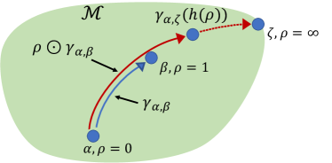
Considering the forward extension of a geodesic, assume that the geodesic extends to the boundary point and denote the extended geodesic by . For , we then define a scalar multiplication by
where
It is straightforward to verify that the start point of is always , while the end point is for and for ; see Figure 1 for an illustration. Similar modifications apply to the reverse extension where . To simplify the notation, we write the end point of as .
Example 2.1 (Space of networks).
Consider simple, undirected, and weighted networks with a fixed number of nodes and bounded edge weights. There is a one-to-one correspondence between such a network and its graph Laplacian. The space of graph Laplacians equipped with the Frobenius (power) metric can thus be used to characterize the space of networks (Zhou and Müller,, 2022), which is a bounded and convex subset of .
Example 2.2 (Space of covariance matrices).
Consider -dimensional covariance matrices with bounded variances. The space of such covariance matrices equipped with the Frobenius distance is a bounded and convex subset of . This holds true for the space of -dimensional correlation matrices as well (Dryden et al.,, 2009).
Example 2.3 (Space of compositional data).
Compositional data takes values in the simplex
reflecting that such data are non-negative proportions that sum to 1. Consider the component-wise square root of an element , the simplex can be mapped to the first orthant of the unit sphere (Scealy and Welsh,, 2011, 2014). We then consider to be the space of compositional data , equipped with the geodesic (Riemannian) metric on the sphere,
This idea can be extended to distributions, where one considers a separable Hilbert space with inner product and norm . The Hilbert sphere is an infinite-dimensional extension of finite-dimensional spheres. The space of (multivariate) absolutely continuous distributions can be equipped with the Fisher-Rao metric
and then modeled as a subset of the Hilbert sphere , where the Fisher-Rao metric pertains to the geodesic metric between square roots of densities and .
Example 2.4 (Wasserstein space).
Consider univariate probability measures on with finite second moments. The space of such probability measures, equipped with the Wasserstein metric , is known as the Wasserstein space , which is a complete and separable metric space. The Wasserstein metric between any two probability measures and is
where , denote the quantile functions of and , respectively.
2.2. Geodesic average treatment effects
Let be a uniquely extendable geodesic metric space. Units are either given a treatment or not treated. For the -th unit, we observe a treatment indicator variable , where if the -th unit is treated and otherwise, along with an outcome
where are potential outcomes for and , respectively. Additionally, we observe Euclidean covariates . We assume that is an i.i.d. sample from a joint distribution , where a generic random variable distributed according to is and we assume that all conditional distributions are well-defined; expectations and conditional expectations in the following are with respect to . We assume that is a compact subset of and write if .
A standard way to quantify causal effects for the usual situation where outcomes are located in Euclidean spaces is to target the difference of the potential outcomes. However, when outcomes take values in a general metric space this is not an option anymore, due to the absence of linear structure in general metric spaces (see, e.g., Example 2.3), which means that the notion of a difference does not exist. This requires to extend the conventional notion of causal effects for the case of random objects in , and to address this challenge we propose here to replace the conventional difference by the geodesic that connects the Fréchet means of the potential outcomes.
Define the Fréchet mean of a random element and the conditional Fréchet mean of given as
| (2.1) |
respectively. Assuming the minimizers are unique and well-defined, we introduce the following notions of causal effects in geodesic metric spaces.
Definition 2.1 (Geodesic individual/average treatment effect).
The geodesic individual treatment effect of on is defined as the geodesic connecting and , i.e., . The geodesic average treatment effect (GATE) of on is defined as the geodesic connecting and , i.e., .
In Euclidean spaces, the geodesic individual treatment effect and geodesic average treatment effect (GATE) reduce to the difference of the potential outcomes for the -th unit, , and the difference of the expected potential outcomes, , respectively. These can be interpreted as the quantities that represent the shortest distance and directional information from to or from to with respect to the Euclidean metric. Since a geodesic connecting points and in a geodesic metric space embodies both the shortest distance and directional information from to with respect to the metric , Definition 2.1 emerges as a natural extension of quantifying treatment effects in geodesic metric spaces.
3. Doubly robust estimation of geodesic average treatment effects
3.1. Preliminaries
To construct doubly robust estimators in metric spaces, one needs to extend the notion of doubly robust estimation of causal effects to the case of random objects in a geodesic metric space. In analogy to the Euclidean case, key ingredients are propensity scores and conditional Fréchet means for the potential outcomes for . We impose the following conditions.
Assumption 3.1.
-
(i)
is a uniquely extendable geodesic metric space that is complete, separable, and totally bounded.
-
(ii)
There exists a constant such that for each .
-
(iii)
and are conditionally independent given .
Assumptions 3.1 (ii) and (iii) are standard overlap and unconfoundedness (or ignorability) conditions in the context of causal inference. Assumption 3.1 (ii) says that for any , there is a positive probability that there are units in both the treatment and control groups in any arbitrarily small neighborhood around . Assumptions 3.1 (iii) says that conditionally on , the treatment is randomly assigned from the potential outcomes. In the Euclidean case, this setup leads to various estimation methods for the average treatment effect, including inverse probability weighting, outcome regression, and doubly robust estimation methods.
Our goal here is to extend the doubly robust estimation to geodesic metric spaces, aiming at GATE (geodesic average treatment effect). To this end, we need to introduce the notion of a (Fréchet) regression model of on in geodesic metric spaces. More precisely, we impose the following conditions, where is as in (2.1).
Assumption 3.2.
There exist random perturbation maps and conditional Fréchet mean functions for such that
-
(i)
,
-
(ii)
,
-
(iii)
.
The random perturbation map is a generalization of additive noise in the Euclidean case that is needed here because the addition operation is not defined, and generalizes the error assumption . Specifically, Assumption 3.2 (ii) is equivalent to so that becomes the Fréchet regression function of on (Petersen and Müller,, 2019). In the following, we refer to as the outcome regression function. Note that our conditions on the perturbation maps are generalizations of those considered in Chen and Müller, (2022).
To obtain a doubly robust representation of the GATE, we additionally introduce an expectation operation for geodesics. For random objects and Euclidean random variables and , define
These definitions of geodesic expectations , , and are consistent with the corresponding (conditional) expectations in the Euclidean case if and are conditionally independent given . Indeed, if and are conditionally independent given and are Euclidean, it is easy to see that by the law of iterated expectations.
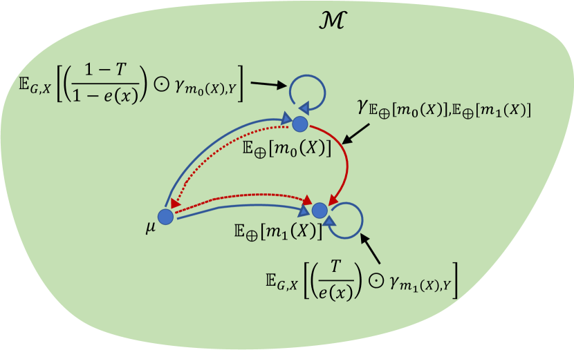
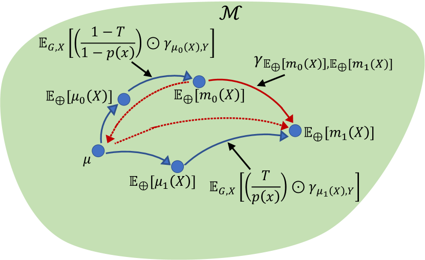
Based on the above assumptions and notions, a doubly robust representation of the GATE for geodesic metric spaces is as follows.
Proposition 3.1.
This proposition shows that the GATE is a natural generalization of the average treatment effect for Euclidean data to the case of geodesic metric spaces (see Remark 3.1 below). Furthermore, we note the double robustness property of the GATE estimator, i.e., either or for could be misspecified (but not both) while still achieving consistent estimation of the GATE. Since the GATE is defined via the geodesic between the Fréchet means for the potential outcomes, we first establish the representation from an arbitrary starting point in (3.1). Although the representation of the GATE in (3.2) also involves an arbitrary starting point , the doubly robust, cross-fitting, and outcome regression GATE estimators presented below do not require to choose ; however, implementing the inverse probability weighting estimator requires choice of a starting point that can be arbitrary (see Remark 3.3 below for further details). We illustrate in Figure 2 the doubly robust representation of the GATE when the outcome regression model or alternatively the propensity score model is correctly specified.
Remark 3.1 (Connection with the established doubly robust estimator for Euclidean data).
For the Euclidean case, , where is the standard Euclidean metric. Then the average treatment effect of the treatment on the outcome is and Assumption 3.1 guarantees
| (3.3) |
provided or for and this leads to the construction of a doubly robust estimator for the Euclidean case. Additionally, we can show that for any ,
| (3.4) |
Adopting this perspective, Proposition 3.1 is seen to be indeed an extension of the doubly robust representation for the average treatment effect in the Euclidean setting to geodesic metric spaces, with the Euclidean scenario as a special case; see Appendix C for the proof of (3.1).
3.2. Doubly robust estimation
Building upon Proposition 3.1, we can construct a sample based doubly robust estimator for the GATE. Note that the right-hand side of (3.2) can be rewritten as with
which corresponds to the representation in (3.1). By moving to the sample counterpart, a doubly robust estimator for the GATE is obtained as , where
| (3.5) |
Here is a parametric model for the propensity score , is an estimator of , and is an estimator of the outcome regression function . In our real data analysis, we estimate the propensity score by the logistic regression model and the outcome regression function by global Fréchet regression (Petersen and Müller,, 2019):
| (3.6) |
where , is the sample size of , , and .
Remark 3.2 (Cross-fitting estimator).
In the Euclidean case, doubly robust estimation methods have been combined with the cross-fitting approach to mitigate over-fitting (Chernozhukov et al.,, 2018). The proposed doubly robust estimator can be similarly adapted to incorporate cross-fitting. Details are as follows.
Let be a (random) partition of into subsets. For each , let and be the estimators of and computed from the data falling into the -th subset, where . Setting
where is the sample size of , the cross-fitting doubly robust estimator for the GATE is obtained as , with
| (3.7) |
In the next section, we provide the asymptotic properties of these doubly robust and cross-fitting sample based estimators.
Remark 3.3 (Outcome regression and inverse probability weighting estimators).
If the models for the outcome regression functions are correctly specified, i.e., , we obtain and the GATE can be estimated by taking a sample counterpart of , which we refer to as the outcome regression estimator. Specifically, the outcome regression estimator for the GATE is given by , where
On the other hand, if the model for the propensity score is correctly specified, i.e., , one finds
for any . Thus the GATE can be obtained by using the inverse probability weighting method, which corresponds to the sample counterpart of
| (3.8) |
Specifically, since (3.8) can be rewritten as with
the inverse probability weighting estimator for the GATE is given by , where
and is an estimator of . While the inverse probability weighting estimator requires the choice of a starting point of a geodesic in (3.8), this starting point can be arbitrarily chosen; a simple choice that we adopt in our implementations is , the sample Fréchet mean of the . The asymptotic properties of and are provided in Appendix A and the finite sample performance of the outcome regression and inverse probability weighting estimators is examined through simulations in Section 5.
4. Main results
4.1. Consistency and convergence rates
To examine the asymptotic properties of the proposed doubly robust and cross-fitting estimators, we impose the following assumptions on the models for the propensity score and outcome regression functions. Let be a class of parametric models for the propensity score , where is a compact set. For , let be an estimator for the outcome regression function .
Assumption 4.1.
-
(i)
For , assume that for some positive constant , and for all and , where is the same constant as in Assumption 3.1(ii).
-
(ii)
There exists and an estimate such that with as .
-
(iii)
There exist functions , such that , with as .
Assumptions 4.1 (i) and (ii) imply the uniform convergence rate for the propensity score estimator, , regardless of whether the propensity score model is misspecified or not. These assumptions are typically satisfied with under mild regularity conditions. Assumption 4.1 (iii) concerns the outcome regression. If one employs the global Fréchet regression model (3.6) for estimating , then under some regularity conditions, this assumption is satisfied with for some (see Theorem 1 in Petersen and Müller, (2019)) and
where , again regardless of whether the model is misspecified or not for the conditional Fréchet mean, which is the true target. Alternatively, one can employ local Fréchet regression as outcome regression method, which is more flexible but comes with slower rates of convergence and is subject to the curse of dimensionality (see Theorem 1 in Chen and Müller, (2022)).
To establish the consistency of and in (3.2) and (3.7), we additionally require that the geodesics in satisfy the following assumption.
Assumption 4.2.
For all ,
| (4.1) |
for some positive constant depending only on .
This is a Lipschitz-type condition to control the criterion function (3.2) that involves the geodesics . When the space is a CAT() space (i.e., a geodesic metric space that is globally non-positively curved in the sense of Alexandrov), this assumption is automatically satisfied. Many metric spaces of statistical interest are CAT() spaces, such as the Wasserstein space of univariate distributions, the space of networks expressed as graph Laplacians with the (power) Frobenius metric, covariance/correlation matrices with the affine-invariant metric (Thanwerdas and Pennec,, 2023), the Cholesky metric (Lin,, 2019) and various other metrics (Pigoli et al.,, 2014), as well as phylogenetic tree space with the BHV metric (Billera et al.,, 2001; Lin and Müller,, 2021). Assumption 4.2 also holds for some relevant positively curved spaces such as open hemispheres or orthants of spheres that are relevant for compositional data with the Riemannian metric; these spaces are not CAT(0), see Example 2.3.
For , denote by the minimizer of the population criterion function, where
To guarantee the identification of the object of interest by the doubly robust estimation approach, we add the following conditions.
Assumption 4.3.
Assume that for ,
-
(i)
the objects and exist and are unique, and for any ,
-
(ii)
.
Assumption 4.3 (i) is a standard separation condition to achieve the consistency of the M-estimator (see, e.g., Chapter 3.2 in van der Vaart and Wellner, (2023)). Note that the existence of the minimizers follows immediately if is compact. Assumption 4.3 (ii) requires that at least one of the models for the propensity score and the outcome regression is correctly specified.
The following result provides the consistency of the doubly robust and cross-fitting estimators in (3.2) and in (3.7).
Theorem 4.1.
To obtain rates of convergence for estimators and in the metric space we need additional entropy conditions to quantify the complexity of the space. Let be the ball of radius centered at and its covering number using balls of size .
Assumption 4.4.
For ,
-
(i)
As ,
(4.2) (4.3) for some and , where for , .
-
(ii)
There exist positive constants , and such that
(4.4)
These assumptions are used to control the behavior of the (centered) criterion function around the minimum. Assumption 4.4 (i) postulates an entropy condition for and . A sufficient condition for (4.3) is for some positive constants and . One can verify (4.2) and
| (4.5) |
for common metric spaces including Examples 2.1–2.4, for which therefore Assumption 4.4 (i) is satisfied. If (4.5) holds, we can take in Theorem 4.2 below arbitrarily small.
Assumption 4.4 (ii) constrains the shape of the population criterion function . This assumption is also satisfied for common metric spaces. Indeed Examples 2.1–2.4 satisfy this condition with (see Propositions B.1–B.4 below). This assumption is an adaptation of Assumption B3 in Delsol and Van Keilegom, (2020) who developed an asymptotic theory for M estimators with plugged-in estimated nuisance parameters. In the Euclidean case, this assumption is typically satisfied with , and the third and fourth terms in (4.4) will be the quadratic and linear terms to approximate the population criterion function for . If does not involve nuisance parameters, the fourth term in (4.4) vanishes, in analogy to Assumption (U2) in Petersen and Müller, (2019).
Under these assumptions, the convergence rates of the doubly robust and cross-fitting estimators are obtained as follows.
Theorem 4.2.
Note that both estimators achieve the same convergence rate. The first term corresponds to the rate for an infeasible estimator, where the nuisance parameters and are known to be contained in neighbors of their (pseudo) true values. If the pseudo true values are completely known, then this term becomes the one with for the conventional Fréchet mean. The second term in the convergence rate is due to the estimation of the nuisance parameters. Generally, neither term dominates. In a typical scenario, we have , , and with any so that the rate becomes for any , which can be arbitrarily close to the parametric rate.
Remark 4.1 (Convergence rates of outcome regression and inverse probability weighting estimators).
In Appendix A, we provide convergence rates of estimators and that rely on the correct specification of the outcome regression function and the propensity score function, respectively. Under some regularity conditions one can show that for each , as ,
where are constants arising from entropy conditions for the models of the outcome regression function and the propensity score, corresponding to in (4.3). Here , , and are null sequences that correspond to the convergence rates of , , and , respectively, i.e.,
4.2. Uncertainty quantification
To obtain uncertainty quantification for the GATE estimators for , we adopt the (adaptive) HulC by Kuchibhotla et al., (2024) to construct confidence regions for the contrast , with implementation as follows.
Let be a (random) partition of into subsets, and estimators for computed for each of the subsamples . Define the maximum median bias of the estimators for as
where .
Adopting the algorithm of HulC, we can construct a confidence interval with coverage probability for as follows:
-
(Step 1)
Find the smallest integer such that
-
(Step 2)
Generate a random variable from the uniform distribution on and set as
-
(Step 3)
Randomly split into disjoint sets and compute .
-
(Step 4)
Compute the confidence interval
5. Simulation studies
5.1. Implementation details and simulation scenarios
The algorithm for the proposed approach is outlined in Algorithm 1. The global Fréchet regression involved in the second step is implemented using the R package frechet (Chen et al.,, 2023). The minimization problem one needs to solve requires specific considerations for various geodesic spaces. For the spaces in Examples 2.1, 2.2, and 2.4, the minimization problem can be reduced to convex quadratic optimization (Stellato et al.,, 2020). For Example 2.3, the necessary optimization can be performed using the trust regions algorithm (Geyer,, 2020). The third step involves the calculation of Fréchet means, which reduces to the entry-wise mean of matrices for Examples 2.1, 2.2, and the mean of quantile functions for Example 2.4 due to the convexity of these spaces. The Fréchet mean for Example 2.3 can be implemented using the R package manifold (Dai,, 2022).
To assess the performance of the proposed doubly robust estimators, we report here the results of simulations for various settings, specifically for the space of covariance matrices equipped with the Frobenius metric and the space of three-dimensional compositional data equipped with the geodesic metric on the sphere ; see Examples 2.2 and 2.3.
We consider sample sizes , with Monte Carlo runs. For the th Monte Carlo run, with denoting the GATE estimator, the average quality of the estimation over the Monte Carlo runs is assessed by the average squared error (ASE)
where is the Frobenius metric for covariance matrices and the geodesic metric for compositional data.
In all simulations, the confounder follows a uniform distribution . The treatment has a conditional Bernoulli distribution depending on with where . We consider two specifications for the outcome regression: a global Fréchet regression model with predictor in (correct specification) and one with the predictor (incorrect specification), and two specifications for the propensity score model: a logistic regression model with predictor (correct specification) and a model with predictor (incorrect specification). To demonstrate the double robustness of estimators and , we compare them with outcome regression (OR) and inverse probability weighting (IPW) estimators.
5.2. Covariance matrices
Random covariance matrices are generated as follows. First, the lower-triangular entries of are independently generated as , where and is independently generated from a uniform distribution on . Due to symmetry, the upper-triangular entries of are then for . To ensure positive semi-definiteness, the diagonal entries are set to equal the sum of all off-diagonal entries in the same row, . This construction results in a diagonally dominated matrix, thus guaranteeing positive semi-definiteness.
We aim to estimate the GATE, whose true value is where , and for . Table 1 presents the simulation results for matrices, i.e., for . The ASE of the doubly robust estimator decreases as the sample size increases when either the OR or IPW model is correctly specified, confirming the double robustness property. However, neither the OR nor IPW estimator demonstrates double robustness; their ASEs can be large even with a sample size of 1000 when the corresponding model is misspecified.
| Model | Sample size | Estimator | ||||
|---|---|---|---|---|---|---|
| OR | IPW | DR | CF | OR | IPW | |
| ✓ | ✓ | 100 | 5.837 (8.694) | 5.839 (8.696) | 5.837 (8.690) | 6.289 (9.105) |
| 300 | 2.058 (2.860) | 2.057 (2.859) | 2.058 (2.860) | 2.128 (2.946) | ||
| 1000 | 0.610 (0.808) | 0.611 (0.809) | 0.610 (0.808) | 0.639 (0.838) | ||
| ✓ | ✗ | 100 | 5.837 (8.690) | 5.835 (8.687) | 5.837 (8.690) | 31.91 (23.45) |
| 300 | 2.058 (2.860) | 2.057 (2.860) | 2.058 (2.860) | 26.26 (13.37) | ||
| 1000 | 0.610 (0.808) | 0.611 (0.808) | 0.610 (0.808) | 24.02 (7.127) | ||
| ✗ | ✓ | 100 | 9.071 (12.317) | 11.09 (16.19) | 37.40 (26.18) | 6.289 (9.105) |
| 300 | 3.005 (3.848) | 3.098 (4.061) | 30.82 (14.19) | 2.128 (2.946) | ||
| 1000 | 0.986 (1.180) | 0.993 (1.201) | 28.23 (7.680) | 0.639 (0.838) | ||
5.3. Compositional data
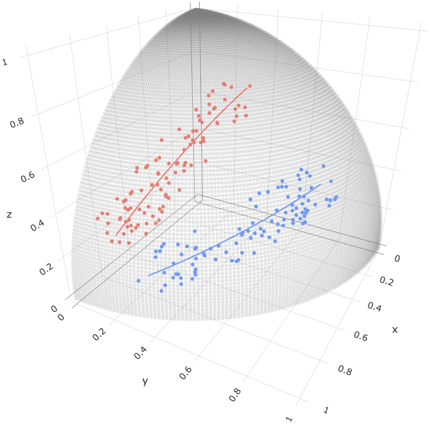
Writing , we model the true regression functions and as
which are illustrated in Figure 3 as red and blues lines, respectively. The random response on for is then generated by adding a small perturbation to the true regression function. To this end, we first construct an orthonormal basis for the tangent space on where
Consider random tangent vectors , where are two independent uniformly distributed random variables on . The random response is obtained as the exponential map at applied to the tangent vector ,
A similar generation procedure is used for , where the orthonormal basis for the tangent space on is
Figure 3 illustrates randomly generated responses using the above generation procedure for a sample size , which are seen to be distributed around the true regression functions.
We are interesting in estimating the GATE, with true value , where
Table 2 summarizes the simulation results. The ASE of the doubly robust estimator decreases as the sample size increases when either the OR or IPW model is correct, thus again confirming the double robustness property. In comparison, neither the OR nor IPW estimator exhibits the double robustness property: When the corresponding model is misspecified, their ASEs do not converge as the sample size increases.
| Model | Sample size | Estimator | ||||
|---|---|---|---|---|---|---|
| OR | IPW | DR | CF | OR | IPW | |
| ✓ | ✓ | 100 | 0.044 (0.026) | 0.044 (0.026) | 0.044 (0.026) | 0.067 (0.030) |
| 300 | 0.026 (0.015) | 0.026 (0.015) | 0.026 (0.015) | 0.047 (0.016) | ||
| 1000 | 0.014 (0.008) | 0.014 (0.008) | 0.014 (0.008) | 0.037 (0.009) | ||
| ✓ | ✗ | 100 | 0.044 (0.026) | 0.044 (0.026) | 0.044 (0.026) | 0.105 (0.039) |
| 300 | 0.026 (0.015) | 0.026 (0.015) | 0.026 (0.015) | 0.093 (0.024) | ||
| 1000 | 0.014 (0.008) | 0.014 (0.008) | 0.014 (0.008) | 0.094 (0.014) | ||
| ✗ | ✓ | 100 | 0.061 (0.034) | 0.067 (0.037) | 0.105 (0.042) | 0.067 (0.030) |
| 300 | 0.039 (0.018) | 0.040 (0.019) | 0.096 (0.026) | 0.047 (0.016) | ||
| 1000 | 0.031 (0.011) | 0.031 (0.011) | 0.098 (0.015) | 0.037 (0.009) | ||
6. Real world applications
6.1. U.S. electricity generation data
Compositional data are ubiquitous and are not situated in a vector space as they correspond to vectors with non-negative elements that sum to 1; see Example 2.3. Various approaches have been developed to address the inherent nonlinearity of compositional data (Aitchison,, 1986; Scealy and Welsh,, 2014; Filzmoser et al.,, 2018) which are common in the analysis of geochemical and microbiome data.
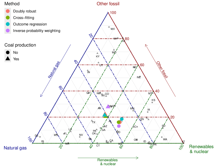
Here we focus on U.S. electricity generation data, publicly available on the U.S. Energy Information Administration website (http://www.eia.gov/electricity). The data reflect net electricity generation from various sources for each state in the year 2020. In preprocessing, we excluded the “pumped storage” and “other” categories due to data errors and consolidated the remaining energy sources into three categories: Natural Gas (corresponding to the category of “natural gas”), Other Fossil (combining “coal,” “petroleum,” and “other gases”), and Renewables and Nuclear (combining “hydroelectric conventional,” “solar thermal and photovoltaic,” “geothermal,” “wind,” “wood and wood-derived fuels,” “other biomass,” and “nuclear”). This yielded a sample of compositional observations taking values in the 2-simplex , as illustrated with a ternary plot in Figure 4. Following the approach described in Example 2.3, we applied the component-wise square root transformation, resulting in compositional outcomes as elements of the sphere , equipped with the geodesic metric.
In our analysis, the exposure (treatment) of interest is whether the state produced coal in 2020, where 29 states produced coal in 2020 while 21 states did not. The outcomes are the compositional data discussed in Example 2.3, where we consider two possible confounders: Gross domestic product (GDP) per capita (millions of chained 2012 dollars) and the proportion of electricity generated from coal and petroleum in 2010 for each state. We implemented the proposed approach to obtain the DR, CF, OR, and IPW estimators, with results demonstrated in Figure 4. The DR, CF, and OR estimators yield similar results, suggesting that coal production leads to a smaller proportion of renewables & nuclear. In contrast, the IPW estimator yields slightly different results, possibly due to the violation of the propensity score model, and therefore should not be used here.
To quantify the size and uncertainty of the treatment effect, we computed the geodesic distance between the two mean potential compositions using the DR estimator and obtained its finite-sample valid confidence region using the adaptive HulC algorithm. Specifically, is found to be 0.133, with the corresponding 95% finite-sample valid confidence region estimated as . This suggests that the effect of coal production on the composition of electricity generation sources is significant at the 0.05 level.
6.2. New York Yellow taxi system after COVID-19 outbreak
Yellow taxi trip records in New York City (NYC), containing details such as pick-up and drop-off dates/times, locations, trip distances, payment methods, and driver-reported passenger counts, can be accessed at https://www.nyc.gov/site/tlc/about/tlc-trip-record-data.page. Additionally, NYC Coronavirus Disease 2019 (COVID-19) data are available at https://github.com/nychealth/coronavirus-data, providing citywide and borough-specific daily counts of probable and confirmed COVID-19 cases in NYC since February 29, 2020.
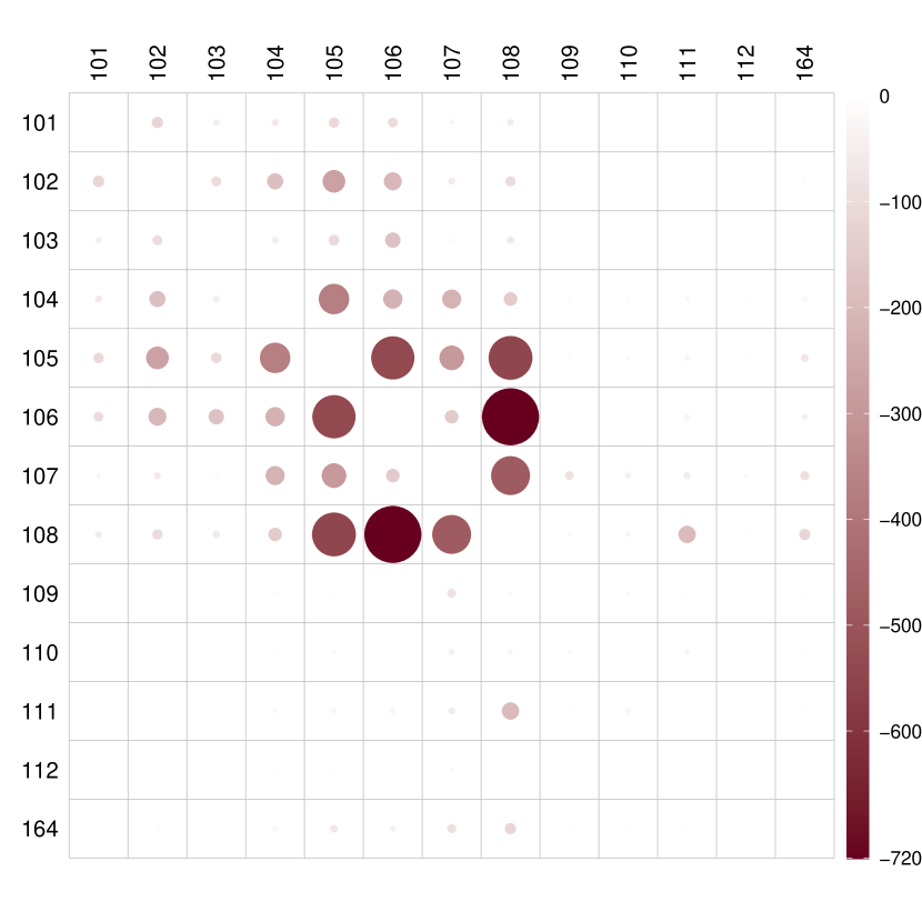
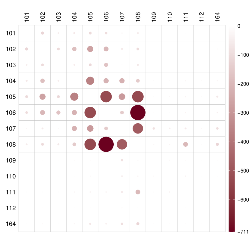
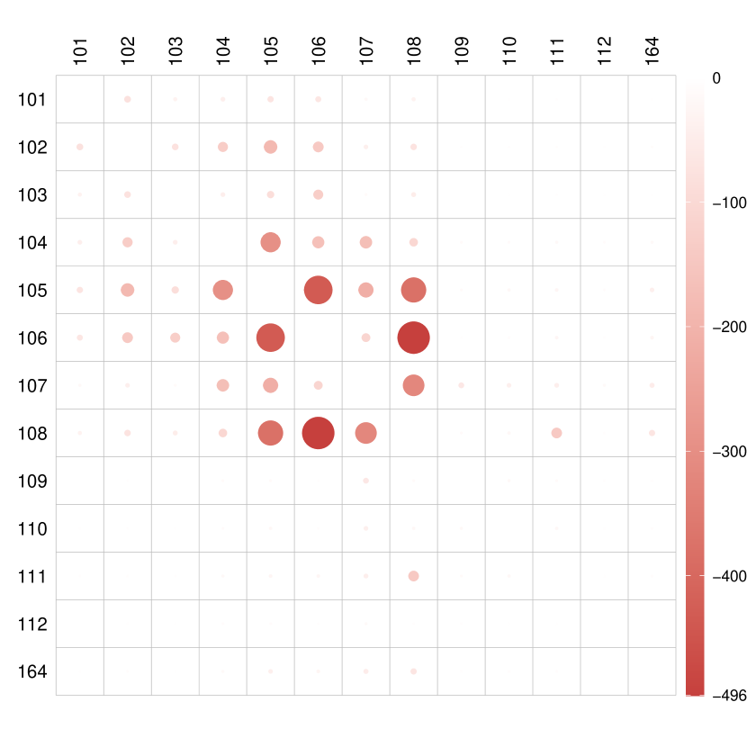
We focused on taxi trip records in Manhattan, which experiences the highest taxi traffic. Following preprocessing procedures outlined in Zhou and Müller, (2022), we grouped the 66 taxi zones (excluding islands) into 13 regions. We restricted our analysis to the period comprising 172 days from April 12, 2020 to September 30, 2020, during which taxi ridership per day in Manhattan steadily increased following a decline due to the COVID-19 outbreak. For each day, we constructed a daily undirected network with nodes corresponding to the 13 regions and edge weights representing the number of people traveling between connected regions. Self-loops in the networks were removed as the focus was on connections between different regions. Thus, we have observations consisting of a simple undirected weighted network for each of the 172 days, each associated with a graph Laplacian.
We aim to investigate the causal effect of COVID-19 new cases on daily taxi networks in Manhattan. COVID-19 new cases were dichotomized into 0 if less than 60 and 1 otherwise, resulting in 79 and 93 days classified into low (0) and high (1) COVID-19 new cases groups, respectively. The outcomes are graph Laplacians as discussed in Example 2.1. Confounders of interest include a weekend indicator and daily average temperature.
We obtained DR and CF estimators using the proposed approach, along with OR and IPW estimators for comparison. In Figure 5, we illustrate the entry-wise differences between the adjacency matrices corresponding to low and high COVID-19 new cases for different estimators. The DR, CF, and OR estimators exhibit similar performance, indicating that high COVID-19 led to less traffic. Regions with the largest differences include regions 105, 106, and 108, primarily residential areas including popular locations such as Penn Station, Grand Central Terminal, and the Metropolitan Museum of Art. The impact of COVID-19 new cases on traffic networks is seen to be negative, especially concerning traffic in residential areas. Conversely, the IPW estimator appears ineffective in capturing this causal effect.
Similarly to Section 6.1, the Frobenius distance between the two mean potential networks using the DR estimator is found to be 5216, with a corresponding finite-sample valid confidence region of . This suggests that the effect of COVID-19 new cases on daily taxi networks in Manhattan is significant at the 0.05 level.

6.3. Brain functional connectivity networks and Alzheimer’s disease
Resting-state functional Magnetic Resonance Imaging (fMRI) methodology allows for the study of brain activation and the identification of brain regions exhibiting similar activity during the resting state (Ferreira and Busatto,, 2013; Sala-Llonch et al.,, 2015). In resting-state fMRI, a time series of Blood Oxygen Level Dependent (BOLD) signals are obtained for different regions of interest (ROI). The temporal coherence between pairwise ROIs is typically measured by temporal Pearson correlation coefficients (PCC) of the fMRI time series, forming an correlation matrix when considering distinct ROIs. Alzheimer’s disease has been found to be associated with anomalies in the functional integration and segregation of ROIs (Zhang et al.,, 2010; Damoiseaux et al.,, 2012).
Our study utilized data obtained from the Alzheimer’s Disease Neuroimaging Initiative (ADNI) database (adni.loni.usc.edu). The dataset in our analysis consists of 372 cognitively normal (CN), and 145 Alzheimer’s (AD) subjects. We used the automated anatomical labeling (AAL) atlas (Tzourio-Mazoyer et al.,, 2002) to parcellate the whole brain into 90 ROIs, with 45 ROIs in each hemisphere, so that The preprocessing of the BOLD signals was implemented by adopting standard procedures of slice-timing correction, head motion correction, and other standard steps. A PCC matrix was calculated for all time series pairs for each subject. These matrices were then converted into simple, undirected, weighted networks by setting diagonal entries to 0 and thresholding the absolute values of the remaining correlations. Density-based thresholding was employed, where the threshold varied from subject to subject to achieve a desired, fixed connection density. Specifically, we retained the 15% strongest connections.
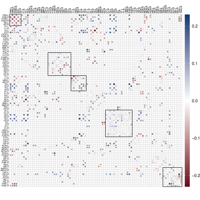
In our analysis, Alzheimer’s disease, coded as a binary variable (0 for cognitively normal, 1 for diagnosed with Alzheimer’s disease), serves as exposure of interest. The outcomes are brain functional connectivity networks, where two confounders are the age and gender of each subject. To quantify the impact of Alzheimer’s disease on brain functional connectivity, we computed the entry-wise differences between the adjacency matrices of the two mean potential networks for the DR estimator, as depicted in Figure 6. Our observations reveal that Alzheimer’s disease leads to notable effects on various regions of the human brain. Specifically, the central region, orbital surface in the frontal lobe, temporal lobe, occipital lobe, and subcortical areas exhibit more pronounced influences, displaying clustered patterns consistent with findings in previous literature (Planche et al.,, 2022). Notably, damage to the frontal lobe is associated with issues in judgment, intelligence, and behavior, while damage to the temporal lobe can impact memory.
To assess structural changes in brain functional connectivity networks following Alzheimer’s disease, Table 3 provides a summary of commonly adopted network measures that quantify functional integration and segregation, with definitions provided in Rubinov and Sporns, (2010). Our observations indicate a decrease in all functional integration and segregation measures of brain functional connectivity networks, with local efficiency experiencing the most substantial reduction. Functional segregation, denoting the brain’s ability for specialized processing within densely interconnected groups of regions, and functional integration, representing the capacity to rapidly combine specialized information from distributed brain regions, are both compromised. This finding implies that Alzheimer’s disease leads to lower global and local efficiency in human brains, disrupting crucial functions such as judgment and memory (Ahmadi et al.,, 2023).
| Cognitively normal | Alzheimer’s disease | ||
|---|---|---|---|
| Functional integration | Global efficiency | 3.117 | 2.914 |
| Characteristic path length | 10.319 | 9.593 | |
| Functional segregation | Local efficiency | 3.599 | 3.035 |
| Clustering coefficient | 0.154 | 0.142 |
7. Discussion
We mention here a few additional issues. Although our assumptions are satisfied for most metric spaces of interest and guarantee relatively fast convergence rates of the proposed doubly robust estimators, one may consider alternative assumptions. For example, one can replace Assumption 4.4 (ii) with an analogous condition as Assumption (U2) in Petersen and Müller, (2019), that is
However, under this relaxed assumption, the convergence rates of the estimators and will be slower than those reported in Theorem 4.2. Specifically, the term would need to be replaced with .
Even when objects that represent outcomes of interest are given, for example covariance matrices, there is still the issue of choosing a metric and ensuing geodesics, where interpretability of the resulting GATE will be a consideration. For a brief discussion of this and related issues, see Dubey et al., (2024).
There are numerous scenarios where metric space-valued outcomes are of interest in causal inference, as we have demonstrated in our empirical examples. Our tools to construct estimators for treatment effects are inspired by their linear counterparts but are substantially different, and notions of Euclidean treatment effects need to be revisited to arrive at canonical generalizations for metric spaces. These investigations also shed new light on and lead to a reinterpretation of the conventional Euclidean case. Future exploration of technical aspects and real world applications for object data will enhance the applicability of causal inference methods across a range of complex data.
Appendix A Asymptotic properties of OR and IPW estimators
A.1. Outcome regression
In this section, we provide asymptotic properties of outcome regression estimators.
Assumption A.1.
Let , be estimators for the outcome regression functions , . Assume that , with as .
Assumption A.2.
Define where . The objects and exist and are unique, and for any , .
Assumption A.3.
For ,
-
(i)
As ,
(A.1) (A.2) for some and .
-
(ii)
There exist positive constants , , , , and such that
A.2. Inverse probability weighting
In this section, we provide asymptotic properties of inverse probability weighting estimators.
Assumption A.4.
Let and be estimators for and the propensity score , respectively. Assume that and with as .
Assumption A.5.
Define where
Assume that and the objects and exist and are unique, and for any , .
Assumption A.6.
For ,
-
(i)
As ,
(A.5) (A.6) for some and , where for , .
-
(ii)
There exist positive constants , , , , and such that
Appendix B Verification of Model Assumptions
Proposition B.1.
Proof.
Note that the geodesic in the space of graph Laplacians (equipped with the Frobenius metric) is simply the line segment connecting the two endpoints. It is easy to verify that Assumption 4.2 holds for . Following the argument in Theorem 2 of Zhou and Müller, (2022), one can verify that Assumptions 4.3 (i) and 4.4 hold with in Assumption 4.4 (ii). Assumption 3.1(i) holds as the space of graph Laplacians is a bounded and closed subset of (cf. Proposition 1 of Zhou and Müller, (2022)).
To prove that Assumptions 3.2 (ii) and (iii) hold, observe that we can define the perturbation of by adding errors component-wise to , , where is an random graph Laplacian with for . The definition of the perturbation map implies Assumption 3.2 (ii). Let denote the trace of the matrix . For any graph Laplacian , we have , which implies Assumption 3.2 (iii). ∎
Proposition B.2.
Proposition B.3.
Consider the space of compositional data defined in Example 2.3. Let be the tangent bundle at and let and denote exponential and logarithmic maps at , respectively. Define and , where
Additionally, for and , define . If there exist positive constants and such that
| (B.1) |
then the space satisfies Assumptions 3.1(i), 3.2(ii), (iii), 4.2, 4.3(i), and 4.4, where is the smallest eigenvalue of a square matrix .
Proof.
Assumption 4.2 holds trivially for . So we verify Assumption 4.2 for . Note that for any , we have , which implies the equivalence of the geodesic metric and the ambient Euclidean metric. One can find a positive constant depending only on such that and this yields (4.1) with .
Following the argument in Proposition 3 of Petersen and Müller, (2019), one can verify that Assumptions 4.3 (i) and 4.4 hold with in Assumption 4.4 (ii) under (B.1). Assumption 3.1 (i) holds as is a bounded and closed subset of the unit sphere .
For any , define the perturbation of as a perturbation in the tangent space, , where is a random tangent vector where denotes the orthonormal basis for the tangent space on and are real-valued independent random variables with mean zero. Since , it follows that and thus Assumption 3.2 (ii) holds. One can similarly show that Assumption 3.2 (iii) is satisfied.
∎
Proposition B.4.
Proof.
For any probability measure , the map is an isometry from to the subset of the Hilbert space formed by equivalence classes of left-continuous nondecreasing functions on . The Wasserstein space can thus be viewed as a convex and closed subset of (Bigot et al.,, 2017). The corresponding Wasserstein metric aligns with the metric between quantile functions. It is straightforward to verify that Assumption 4.2 is satisfied for the Hilbert space with . Since the Wasserstein space is a closed subset of , the geodesic extension necessitates adjustments to prevent boundary crossings, as discussed in Section 2. Such adjustments can only reduce the left-hand side of (4.1), thereby ensuring that Assumption 4.2 holds for . Assumption 3.1(i) holds as the Wasserstein space is a bounded and closed subset of . Following the argument in Proposition 1 of Petersen and Müller, (2019), one can verify that Assumptions 4.3 (i) and 4.4 hold with in Assumption 4.4 (ii).
Appendix C Proofs for Section 3
C.1. Proof of Proposition 3.1
Step 1. It is sufficient to check (3.2) when
-
(i)
the propensity score is correctly specified, that is, (Step 2) or
-
(ii)
the outcome regression functions are correctly specified, that is, , (Step 3).
Now we provide some auxiliary results. Observe that
This yields
Then we have
| (C.1) |
Likewise, we have
| (C.2) |
Further, for random objects , we have
| (C.3) |
C.2. Proof of (3.1)
Assume that or for . Note that the geodesic in is the line segment connecting two endpoints and any geodesic is extendable, that is, for any , .
Appendix D Proofs for Section 4
For any positive sequences , we write if there is a constant independent of such that for all .
D.1. Proof of Theorem 4.1 (i)
Define . By Corollary 3.2.3 in van der Vaart and Wellner, (2023), it is sufficient to show
where
Now we show ; the proof for is similar. For this, we show that converges weakly to in and then apply Theorem 1.3.6 in van der Vaart and Wellner, (2023). From Theorem 1.5.4 in van der Vaart and Wellner, (2023), this weak convergence follows by showing that
-
(i)
for each as .
-
(ii)
is asymptotically equicontinuous in probability, i.e., for each , there exists such that
For an arbitrary , for (i) we have
and observe that
| (D.1) |
| (D.2) |
| (D.3) |
Pick any . For (ii), similarly to the argument leading to (D.1),
and this implies so that we obtain (ii), which completes the proof.
D.2. Proof of Theorem 4.1 (ii)
Note that one can show by applying similar arguments as in the proof of Theorem 4.1 (i). From the definition of ,
which implies that for some . Then
| (D.4) | ||||
D.3. Proof of Theorem 4.2(i)
Now we show (4.6) when . The case is analogous. We adapt the proof of Theorem 3.2.5 in van der Vaart and Wellner, (2023). Define
For some and , consider the class of functions
for any . An envelope function for is . Observe that
Then for , following Theorem 2.7.17 of van der Vaart and Wellner, (2023), the bracketing number of is bounded by a multiple of , where , and are constants depending only on , , , and .
Assumption 4.4 (i) and Theorem 2.14.16 of van der Vaart and Wellner, (2023) imply that, for small enough ,
| (D.5) |
For any , set and
Choose to satisfy Assumption 4.4 (ii) and also small enough so that Assumption 4.4 (i) holds for all and set . For any ,
| (D.6) |
where .
Note that for any , there exist an integer such that , , and .
Define as with . Then, on , for each fixed such that , one has for all ,
Then for large such that , we have
| (D.7) |
D.4. Proof of Theorem 4.2(ii)
References
- Ahmadi et al., (2023) Ahmadi, H., Fatemizadeh, E., and Motie-Nasrabadi, A. (2023). A comparative study of correlation methods in functional connectivity analysis using fMRI data of Alzheimer’s patients. Journal of Biomedical Physics & Engineering, 13(2):125.
- Aitchison, (1986) Aitchison, J. (1986). The Statistical Analysis of Compositional Data. Chapman & Hall, Ltd.
- Athey and Imbens, (2017) Athey, S. and Imbens, G. W. (2017). The state of applied econometrics: Causality and policy evaluation. Journal of Economic Perspectives, 31(2):3–32.
- Bang and Robins, (2005) Bang, H. and Robins, J. M. (2005). Doubly robust estimation in missing data and causal inference models. Biometrics, 61(4):962–973.
- Bigot et al., (2017) Bigot, J., Gouet, R., Klein, T., and López, A. (2017). Geodesic PCA in the Wasserstein space by convex PCA. Annales de l’Institut Henri Poincaré B: Probability and Statistics, 53:1–26.
- Billera et al., (2001) Billera, L. J., Holmes, S. P., and Vogtmann, K. (2001). Geometry of the Space of Phylogenetic Trees. Advances in Applied Mathematics, 27:733–767.
- Chen and Müller, (2022) Chen, Y. and Müller, H.-G. (2022). Uniform convergence of local Fréchet regression with applications to locating extrema and time warping for metric space valued trajectories. Annals of Statistics, 50(3):1573–1592.
- Chen et al., (2023) Chen, Y., Zhou, Y., Chen, H., Gajardo, A., Fan, J., Zhong, Q., Dubey, P., Han, K., Bhattacharjee, S., Zhu, C., Iao, S. I., Kundu, P., Petersen, A., and Müller, H.-G. (2023). frechet: Statistical Analysis for Random Objects and Non-Euclidean Data. R package version 0.3.0.
- Chernozhukov et al., (2018) Chernozhukov, V., Chetverikov, D., Demirer, M., Duflo, E., Hansen, C., Newey, W., and Robins, J. (2018). Double/debiased machine learning for treatment and structural parameters. The Econometrics Journal, 21(1):C1–C68.
- Dai, (2022) Dai, X. (2022). Statistical Inference on the Hilbert Sphere with Application to Random Densities. Electronic Journal of Statistics, 16(1):700–736.
- Damoiseaux et al., (2012) Damoiseaux, J. S., Prater, K. E., Miller, B. L., and Greicius, M. D. (2012). Functional connectivity tracks clinical deterioration in Alzheimer’s disease. Neurobiology of Aging, 33(4):828–e19.
- Delsol and Van Keilegom, (2020) Delsol, L. and Van Keilegom, I. (2020). Semiparametric m-estimation with non-smooth criterion functions. Annals of the Institute of Statistical Mathematics, 72(2):577–605.
- Dryden et al., (2009) Dryden, I. L., Koloydenko, A., and Zhou, D. (2009). Non-Euclidean statistics for covariance matrices, with applications to diffusion tensor imaging. Annals of Applied Statistics, 3:1102–1123.
- Dubey et al., (2024) Dubey, P., Chen, Y., and Müller, H.-G. (2024). Metric statistics: Exploration and inference for random objects with distance profiles. Annals of Statistics, 52:757–792.
- Ferreira and Busatto, (2013) Ferreira, L. K. and Busatto, G. F. (2013). Resting-state functional connectivity in normal brain aging. Neuroscience & Biobehavioral Reviews, 37(3):384–400.
- Filzmoser et al., (2018) Filzmoser, P., Hron, K., and Templ, M. (2018). Applied Compositional Data Analysis: With Worked Examples in R. Springer.
- Gallier and Quaintance, (2020) Gallier, J. and Quaintance, J. (2020). Differential Geometry and Lie Groups: A Computational Perspective, volume 12. Springer.
- Geyer, (2020) Geyer, C. J. (2020). trust: Trust Region Optimization. R package version 0.1.8.
- Gunsilius, (2023) Gunsilius, F. F. (2023). Distributional synthetic controls. Econometrica, 91(3):1105–1117.
- Hahn, (1998) Hahn, J. (1998). On the role of the propensity score in efficient semiparametric estimation of average treatment effects. Econometrica, pages 315–331.
- Hirano et al., (2003) Hirano, K., Imbens, G. W., and Ridder, G. (2003). Efficient estimation of average treatment effects using the estimated propensity score. Econometrica, 71(4):1161–1189.
- Imbens and Rubin, (2015) Imbens, G. W. and Rubin, D. B. (2015). Causal Inference in Statistics, Social, and Biomedical Sciences. Cambridge university press.
- Kuchibhotla et al., (2024) Kuchibhotla, A. K., Balakrishnan, S., and Wasserman, L. (2024). The HulC: Confidence regions from convex hulls. Journal of the Royal Statistical Society Series B Statistical Methodology, In press.
- Lin, (2019) Lin, Z. (2019). Riemannian geometry of symmetric positive definite matrices via Cholesky decomposition. SIAM Journal on Matrix Analysis and Applications, 40(4):1353–1370.
- Lin et al., (2023) Lin, Z., Kong, D., and Wang, L. (2023). Causal inference on distribution functions. Journal of the Royal Statistical Society Series B: Statistical Methodology, 85(2):378–398.
- Lin and Müller, (2021) Lin, Z. and Müller, H.-G. (2021). Total variation regularized Fréchet regression for metric-space valued data. Annals of Statistics, 49:3510–3533.
- McCann, (1997) McCann, R. J. (1997). A convexity principle for interacting gases. Advances in Mathematics, 128(1):153–179.
- Peters et al., (2017) Peters, J., Janzing, D., and Schölkopf, B. (2017). Elements of Causal Inference: Foundations and Learning Algorithms. The MIT Press.
- Petersen and Müller, (2019) Petersen, A. and Müller, H.-G. (2019). Fréchet regression for random objects with Euclidean predictors. Annals of Statistics, 47(2):691–719.
- Pigoli et al., (2014) Pigoli, D., Aston, J. A., Dryden, I. L., and Secchi, P. (2014). Distances and inference for covariance operators. Biometrika, 101:409–422.
- Planche et al., (2022) Planche, V., Manjon, J. V., Mansencal, B., Lanuza, E., Tourdias, T., Catheline, G., and Coupé, P. (2022). Structural progression of Alzheimer’s disease over decades: the MRI staging scheme. Brain Communications, 4(3):fcac109.
- Robins et al., (1994) Robins, J. M., Rotnitzky, A., and Zhao, L. P. (1994). Estimation of regression coefficients when some regressors are not always observed. Journal of the American statistical Association, 89(427):846–866.
- Rosenbaum and Rubin, (1983) Rosenbaum, P. R. and Rubin, D. B. (1983). The central role of the propensity score in observational studies for causal effects. Biometrika, 70(1):41–55.
- Rubinov and Sporns, (2010) Rubinov, M. and Sporns, O. (2010). Complex network measures of brain connectivity: Uses and interpretations. NeuroImage, 52(3):1059–1069.
- Sala-Llonch et al., (2015) Sala-Llonch, R., Bartrés-Faz, D., and Junqué, C. (2015). Reorganization of brain networks in aging: A review of functional connectivity studies. Frontiers in Psychology, 6.
- Scealy and Welsh, (2011) Scealy, J. and Welsh, A. (2011). Regression for compositional data by using distributions defined on the hypersphere. Journal of the Royal Statistical Society: Series B (Statistical Methodology), 73(3):351–375.
- Scealy and Welsh, (2014) Scealy, J. and Welsh, A. (2014). Colours and cocktails: Compositional data analysis. Australian & New Zealand Journal of Statistics, 56(2):145–169.
- Scharfstein et al., (1999) Scharfstein, D. O., Rotnitzky, A., and Robins, J. M. (1999). Adjusting for nonignorable drop-out using semiparametric nonresponse models. Journal of the American Statistical Association, 94(448):1096–1120.
- Stellato et al., (2020) Stellato, B., Banjac, G., Goulart, P., Bemporad, A., and Boyd, S. (2020). OSQP: An operator splitting solver for quadratic programs. Mathematical Programming Computation, 12(4):637–672.
- Thanwerdas and Pennec, (2023) Thanwerdas, Y. and Pennec, X. (2023). O(n)-invariant Riemannian metrics on SPD matrices. Linear Algebra and its Applications, 661:163–201.
- Tzourio-Mazoyer et al., (2002) Tzourio-Mazoyer, N., Landeau, B., Papathanassiou, D., Crivello, F., Etard, O., Delcroix, N., Mazoyer, B., and Joliot, M. (2002). Automated anatomical labeling of activations in SPM using a macroscopic anatomical parcellation of the MNI MRI single-subject brain. NeuroImage, 15(1):273–289.
- van der Vaart and Wellner, (2023) van der Vaart, A. W. and Wellner, J. A. (2023). Weak Convergence and Empirical Processes with Applications to Statistics. Springer.
- Zhang et al., (2010) Zhang, H.-Y., Wang, S.-J., Liu, B., Ma, Z.-L., Yang, M., Zhang, Z.-J., and Teng, G.-J. (2010). Resting brain connectivity: changes during the progress of Alzheimer disease. Radiology, 256(2):598–606.
- Zhou and Müller, (2022) Zhou, Y. and Müller, H.-G. (2022). Network regression with graph Laplacians. Journal of Machine Learning Research, 23:1–41.
- Zhu and Müller, (2023) Zhu, C. and Müller, H.-G. (2023). Geodesic optimal transport regression. arXiv preprint arXiv:2312.15376.