Geodesic deviation on symmetry axis in Taub–NUT metric

Within the framework of general relativity many questions about the structure of spacetime are often reduced to solving problems on the behavior of geodesic curves in a certain metric. One way to investigate the properties of geodesics is to consider the geodesic deviation equation, which describes the relative acceleration of two close geodesics. This acceleration is often interpreted synonymously with the tidal one.

Historically, the first static solution to Einstein’s equations was the Schwarzschild solution [1], which describes the spherically symmetric gravitational field of a massive object. Geodesic deviation equation was considered in Schwarzschild metric in [2], solutions were found for radial geodesics in terms of elementary functions. It was shown that only radial component of geodesic deviation vector tends to infinity near a physical singularity. Which means unlimited growth of radial tidal force component acting on a freely falling body. Natural generalizations of the Schwarzschild solution were Reissner–Nordström metric [3], [4] and Kottler metric [5] (which is more often called Schwarzschild–(Anti)-De Sitter metric). The geodesic deviation equation in these metrics is considered in the works [6] and [7] respectively. The article [8] tells about tidal properties near black hole surrounded quintessence, which is called Kiselev black hole [9].

Tidal effects play a critical role in many astrophysical phenomena. For example, tidal disruption event (or tidal disruption flare) is that the star is destructed by supermassive black hole gravity. Tidal forces acting on a star in the Schwarzschild gravitational field are studied in [10]. It should also be noted that the relative tidal acceleration between the two gravitational wave detectors was used to study graviton properties [11], [12].

It is also worth noting that there are quite interesting works also devoted to the study of geodesic deviation equation in static spherically symmetric spacetimes: Ref. [13] is about tidal force near the naked singularity, Refs. [14] and [15] are about tidal effects in regular black holes, Ref. [16] generalized geodesic deviation description of Schwarzschild spacetime with holographic massive gravity, Ref. [17] shows properties of the relative geodesic motion in 4D Einstein–Gauss–Bonnet black hole. In [18] was considered tidal effects in the vicinity of null naked singularity spacetime. And article [19] is about tidal properties of a black hole surrounded by dark matter halo.

But a particularly important class of static metrics is the spacetimes of axial symmetry. Among them are metric of massive rotating Kerr black hole [20], vacuum static axial symmetry Taub–NUT spacetime [21], electrically charged Kerr–Newman metric [22]. The article [23] contains geodesic deviation equation analysis on the symmetry axis of Kerr spacetime. The study of tidal effects in axisymmetric spactimes in the vicinity of rotation axis, for example, in the Kerr metric, can make it possible to describe the gravitational principle of astrophysical jets formation. The description of relativistic flow formation in tidal acceleration terms is presented in [24], [25], [26].

It is also should be noted that the geodesic deviation equation finds its application not only in the description of tidal forces, but also in the properties of orbit, which differ little from circular ones. The works [27], [28] and [29] are devoted to the properties of such orbits, and there the so-called Shirokov effect was described in various metrics.

In our work, the main object of research is the geodesic properties of the Taub–NUT spacetime. This metric is very interesting because, on the one hand, like the Kerr metric, it is an axially symmetric generalization of the Schwazschild metric, and on the other hand, it is somewhat simpler than the Kerr metric, because $g_{tt}$ and $g_{rr}$ metric components are independent on the polar and azimuthal angles, unlike the Kerr metric. We consider the geodesic deviation equation along the symmetry axis of spacetime because this particular case allows us to eliminate the dynamics of geodesics along the azimuthal direction. This paper is organized as follows. In Sec. 2 we demonstrate Taub–NUT metric and its horizons. Sec. 3 contains geodesic equations and there we restrict the set of all geodesics to the set of on symmetry axis geodesics without azimuthal dynamics. In Sec. 4 we directly discuss the geodesic deviation equation, construct a set of Carter tetrads that allows us to diagonalize the tidal tensor. We also show the areas of tidal compression or extension and regions of growth and decrease of the tidal force components. In Sec. 5 we solve geodesic deviation equations with respect to the radial variable analytically and numerically to illustrate the behavior of geodesic deviation vector components. Final Sec. 6 ends this paper, there we give an interpretation of the obtained calculations and also indicate potential directions for the development of tidal effects studies.

We use signature of the metric $(+,-,-,-)$ and set Newtonian gravitational constant $G$ and light speed $c$ to $1$ throughout this paper.

Taub–NUT metric is an interesting vacuum generalization of Schwarzschild spacetime to the case of axial symmetry. Line element in spherical coordinates is

$$ds^{2}=f(r)\bigg{[}dt+2n\left(1-\cos{\theta}\right)d\phi\bigg{]}^{2}-\frac{dr^{2}}{f(r)}-\left(r^{2}+n^{2}\right)\left(d\theta^{2}+\sin^{2}\theta d\phi^{2}\right),$$

(1)

where

$$f(r)=1-\frac{2Mr+2n^{2}}{r^{2}+n^{2}}$$

(2)

and $n$ is called NUT-charge, $M$ is black hole mass. The horizons are determined by the equation $f(r)=0$ or

$$r^{2}-2Mr-n^{2}=0.$$

(3)

Equation roots are

$$r_{\pm}=M\pm\sqrt{M^{2}+n^{2}}.$$

(4)

But only $r_{+}$ corresponds to the horizon, because $r_{-}<0$ for all values of $n$. To To illustrate the absence of physical singularity at the point $r=0$, one can calculate the curvature invariant Kretschmann scalar

$$\mathcal{K}=R^{\mu\nu\alpha\beta}R_{\mu\nu\alpha\beta}=\frac{48\left(n^{2}-M^{2}\right)\left(n^{6}-15n^{4}r^{2}+15n^{2}r^{4}-r^{6}\right)}{\left(r^{2}+n^{2}\right)^{6}}+\frac{192Mn^{2}r\left(3n^{4}-10n^{2}r^{2}+3r^{4}\right)}{\left(r^{2}+n^{2}\right)^{6}},$$

(5)

which is regular at zero at nonzero NUT-charge

$$\mathcal{K}(0)=\frac{48\left(n^{2}-M^{2}\right)}{n^{2}}.$$

(6)

Using the Hamilton–Jacobi equations, it is easy to obtain the geodesic equations in the Taub–NUT metric

$$\frac{dt}{d\tau}=\frac{E}{f(r)}-2n\left(1-\cos{\theta}\right)\frac{L+2nE\left(1-\cos{\theta}\right)}{\left(r^{2}+n^{2}\right)\sin^{2}{\theta}},$$

(7)

$$\left(\frac{dr}{d\tau}\right)^{2}=E^{2}-f(r)\frac{\delta_{1}r^{2}+L^{2}+K}{\left(r^{2}+n^{2}\right)},$$

(8)

$$\left(\frac{d\theta}{d\tau}\right)^{2}=\frac{K+L^{2}-\delta_{1}n^{2}}{\left(r^{2}+n^{2}\right)^{2}}-\frac{\left(L+2nE(1-\cos{\theta})\right)^{2}}{(r^{2}+n^{2})^{2}\sin^{2}{\theta}},$$

(9)

$$\frac{d\phi}{d\tau}=\frac{L+2nE\left(1-\cos{\theta}\right)}{\left(r^{2}+n^{2}\right)\sin^{2}{\theta}}.$$

(10)

Where $E$ and $L$ are energy and angular momentum of test particle. $K$ is so-called Carter constant, which is the third integral of motion in axially symmetric spacetime, which was for the first time obtained for the Kerr metric [30], and parameter $\tau$ is the proper time, i.e. affine parameter along the geodesic curve. Geodesic equations in Taub–NUT spacetime are discussed in detail in [31]. Parameter $\delta_{1}$ defines the type of geodesics, for timelike geodesics $\delta_{1}=1$, for spacelike geodesics $\delta_{1}=-1$, for lightlike geodesics $\delta_{1}=0$.

The expressions (7)-(10) form a unit covariant 4-velocity vector $u^{\mu}$ tangent to the geodesic.

Before discussing the tidal effects associated with spacetime curvature, it is worth noting that we can define ‘‘Newtoninan acceleration’’ $A^{r}$ as

$$A^{r}=\ddot{r},$$

(15)

which can be found from Eq. (12). It is

$$A^{r}=\delta_{1}\frac{-Mr^{2}+n^{2}(M-2r)}{(r^{2}+n^{2})^{2}},$$

(16)

which gives ‘‘Newtoninan radial acceleration’’ for the Schwarzschild case $n=0$ and massive test body moving along timelike geodesic with $\delta_{1}=1$

$$A^{r}=-\frac{M}{r^{2}}.$$

(17)

When we discuss a particle freely falling from a rest state at $r=r_{0}>r_{+}$, we can indicate the turning point $R^{stop}$ and also show that if it exists then it is unique. Eq. (12) at rest point allows us to determine the energy $E^{2}$ at a distance $r_{0}$ and then this energy will determine another value of the radius $R^{stop}$ at which the speed will be equal to zero again. Thus it is

$$R^{stop}=\frac{n^{2}\left(M-r_{0}\right)}{Mr_{0}+n^{2}}.$$

(18)

It is easy to show that $R^{stop}$ is less than $r_{+}$ for any $r_{0}$. This means that the speed of a freely falling body can reach zero only under the black hole horizon.

The main object of research in this work is the geodesic deviation equation

$$\frac{D^{2}\tilde{\xi}^{\mu}}{d\tau^{2}}=R^{\mu}_{.\nu\alpha\beta}u^{\nu}u^{\alpha}\tilde{\xi}^{\beta},$$

(19)

where $\frac{D^{2}}{d\tau^{2}}$ is covariant derivative along the geodesic, $R^{\mu}_{.\nu\alpha\beta}$ is Riemann curvature tensor and $u^{\mu}$ is the unit 4-velocity vector tangent to the geodesic defined in (7)-(10) and in particular along the axis in (11)-(14). $\tilde{\xi}^{\mu}$ is geodesic deviation vector, which describes the distance between points on adjacent geodesics corresponding to the same value of the affine parameter $\tau$.

Eq. (19) determines the evolution of the $\tilde{\xi}^{\mu}$ vector and describes the movement of geodesics relative to each other. Tidal effects in various gravitational fields are described using the geodesic deviation equation in the general theory of relativity. For this reason $R^{\mu}_{.\nu\alpha\beta}u^{\nu}u^{\alpha}$ is called the tidal tensor. To calculate it we present the nonzero components of the Riemann tensor

	$$R^{0}_{.101}=-\frac{f^{\prime\prime}}{2f},\;R^{0}_{.202}=R^{1}_{.212}=-\frac{rf^{\prime}}{2}-\frac{n^{2}f}{r^{2}+n^{2}},\\$$		(20a)
	$$R^{0}_{.102}=-\frac{\sin{\theta}}{1+\cos{\theta}}\frac{d}{dr}\left(\frac{n^{2}f}{r^{2}+n^{2}}\right),\\$$		(20b)
	$$R^{0}_{.113}=2n\sin^{2}\frac{\theta}{2}\left[\frac{f^{\prime\prime}}{f}-\frac{rf^{\prime}}{f\left(r^{2}+n^{2}\right)}-\frac{2n^{2}}{\left(r^{2}+n^{2}\right)^{2}}\right],$$		(20c)
	$$R^{0}_{.123}=\left[2n^{2}\tan^{2}\frac{\theta}{2}+\frac{r^{2}+n^{2}}{f}\right]\frac{d}{dr}\left(\frac{nf\sin{\theta}}{r^{2}+n^{2}}\right),$$		(20d)
	$$R^{0}_{.213}=\left[4n^{2}\tan^{2}\frac{\theta}{2}+\frac{r^{2}+n^{2}}{2f}\right]\frac{d}{dr}\left(\frac{nf\sin{\theta}}{r^{2}+n^{2}}\right),$$		(20e)
	$$R^{0}_{.223}=2n\sin^{2}\frac{\theta}{2}\left[2+\frac{8fn^{2}}{r^{2}+n^{2}}+r\left(r^{2}+n^{2}\right)\frac{d}{dr}\left(\frac{f}{r^{2}+n^{2}}\right)\right],$$		(20f)
	$$R^{0}_{.303}=-\frac{rf^{\prime}\sin^{2}\theta}{2}+\frac{n^{2}f}{r^{2}+n^{2}}\left(\frac{16fn^{2}\sin^{4}\frac{\theta}{2}}{r^{2}+n^{2}}+8rf^{\prime}\sin^{4}\frac{\theta}{2}-\sin^{2}\theta\right),$$		(20g)
	$$R^{0}_{.312}=\left[2n^{2}\tan^{2}\frac{\theta}{2}-\frac{r^{2}+n^{2}}{2f}\right]\frac{d}{dr}\left(\frac{nf\sin{\theta}}{r^{2}+n^{2}}\right),$$		(20h)
	$$R^{1}_{.313}=8n^{2}ff^{\prime\prime}\sin^{4}\frac{\theta}{2}-\sin^{2}\theta\left[\frac{n^{2}f}{r^{2}+n^{2}}+\frac{rf^{\prime}}{2}\right],$$		(20i)
	$$R^{1}_{.323}=\left(r^{2}+n^{2}\right)f\frac{d}{dr}\left(\frac{6n^{2}f\sin\theta\sin^{2}\frac{\theta}{2}}{r^{2}+n^{2}}\right),$$		(20j)
	$$R^{2}_{.323}=\sin^{2}\theta\left[1-f+\frac{4n^{2}f}{r^{2}+n^{2}}\right]+8n^{2}f\sin^{4}\left(\frac{\theta}{2}\right)\frac{rf^{\prime}(r^{2}+n^{2})+2n^{2}f}{(r^{2}+n^{2})^{2}}.$$		(20k)

Where $f$ is function defined in Eq. (2), prime means differentiation with respect to $r$. And the curvature tensor indices take values $(0,1,2,3)$, which correspond to a set of coordinates $(t,r,\theta,\phi)$. It is not difficult to see that on the symmetry axis at $\theta=0$ Riemann tensor components are greatly simplified. And only the components from the Eq. (20a) remain nonzero on the axis.

Therefore, the tidal tensor $R^{\mu}_{.\nu\alpha\beta}u^{\nu}u^{\alpha}$ has the form

$$\begin{pmatrix}\frac{f^{\prime\prime}\left(E^{2}-\delta_{1}f\right)}{2f}&-\frac{Ef^{\prime\prime}\sqrt{E^{2}-\delta_{1}f}}{2f^{2}}&0&0\\ \frac{Ef^{\prime\prime}\sqrt{E^{2}-\delta_{1}f}}{2}&-\frac{E^{2}f^{\prime\prime}}{2f}&0&0\\ 0&0&-\frac{\gamma\delta_{1}}{2\left(r^{2}+n^{2}\right)^{2}}&0\\ \frac{\gamma E^{2}n}{2\left(r^{2}+n^{2}\right)^{3}}&-\frac{\gamma En\sqrt{E^{2}-\delta_{1}f}}{2f\left(r^{2}+n^{2}\right)^{3}}&0&-\frac{\gamma\delta_{1}}{2\left(r^{2}+n^{2}\right)^{2}}\end{pmatrix},$$

(21)

where

$$\gamma=r\left(r^{2}+n^{2}\right)f^{\prime}+2n^{2}f.$$

(22)

So Eq. (19) can be diagonalized using the tetrad basis for free-fall reference frames. Such a basis for an axially symmetric metric is called Carter’s tetrad basis. The procedure for constructing the tetrad basis is described in detail in the appendix of Ref. [23]. Therefore, we give four tetrad vectors

	$$e^{\mu}_{t}=A\left(r^{2}+n^{2}\right)\left(\frac{1}{f},\frac{\sqrt{E^{2}-\delta_{1}f}}{E},0,\frac{n}{r^{2}+n^{2}}\right),$$		(23a)
	$$e^{\mu}_{r}=\left(\frac{\sqrt{E^{2}-\delta_{1}f}}{f\sqrt{\delta_{1}}},\frac{E}{\sqrt{\delta_{1}}},0,0\right),$$		(23b)
	$$e^{\mu}_{\theta}=\left(0,0,\frac{1}{\sqrt{r^{2}+n^{2}}},0\right),$$		(23c)
	$$e^{\mu}_{\phi}=\left(0,0,0,\frac{1}{\sqrt{\left(r^{2}+n^{2}\right)\sin^{2}\theta-16n^{2}f\sin^{4}\frac{\theta}{2}}}\right),$$		(23d)

where

$$A=\frac{E}{\sqrt{\delta_{1}\left(r^{2}+n^{2}\right)^{2}+4E^{2}n^{2}\sin^{2}\frac{\theta}{2}\left[4n^{2}f\sin^{2}\frac{\theta}{2}+(r^{2}+n^{2})\left(1+\sin^{2}\frac{\theta}{2}\right)\right]}}.$$

(24)

Tetrad set (23) satisfy normalization condition $\eta_{\alpha\beta}=e^{\mu}_{\alpha}e^{\nu}_{\beta}g_{\mu\nu}$ and $\eta_{\alpha\beta}$ is Minkowski metric. All of the above allows us to replace the geodesic deviation vector $\tilde{\xi}^{\mu}$ with tetrads from Eqs. (23) as follows

$$\tilde{\xi}^{\mu}=e^{\mu}_{\alpha}\xi^{\alpha}.$$

(25)

Eq. (19) in terms of the vector $\xi^{\alpha}$ reads

$$\ddot{\xi}^{r}=-\frac{\delta_{1}f^{\prime\prime}}{2}\xi^{r},$$

(26)

$$\ddot{\xi}^{a}=-\delta_{1}\left(\frac{rf^{\prime}}{2\left(r^{2}+n^{2}\right)}+\frac{n^{2}f}{\left(r^{2}+n^{2}\right)^{2}}\right)\xi^{a},$$

(27)

where $a=\theta,\phi$ correspond to the angular components of the geodesic deviation vector. The dot denotes the derivative with respect to the $\tau$. And the time component of the geodesic deviation vector has trivial equation $\ddot{\xi}^{t}=0$. Eqs. (26) and (27) demonstrate that lightlike geodesics (at $\delta_{1}=0$) have trivial equations $\ddot{\xi}^{\mu}=0$ for all components $\mu=t,r,\theta,\phi$. Therefore, the main interest for us is timelike geodesics at $\delta_{1}=1$. Components of tidal acceleration in the Taub–NUT metric are

$$\ddot{\xi}^{r}=2\delta_{1}\left[\frac{Mr^{3}+n^{2}\left(3r^{2}-3Mr-n^{2}\right)}{(r^{2}+n^{2})^{3}}\right]\xi^{r},$$

(28)

$$\ddot{\xi}^{a}=-\delta_{1}\left[\frac{Mr^{3}+n^{2}\left(3r^{2}-3Mr-n^{2}\right)}{(r^{2}+n^{2})^{3}}\right]\xi^{a}.$$

(29)

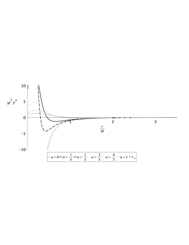
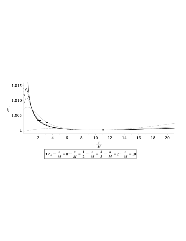
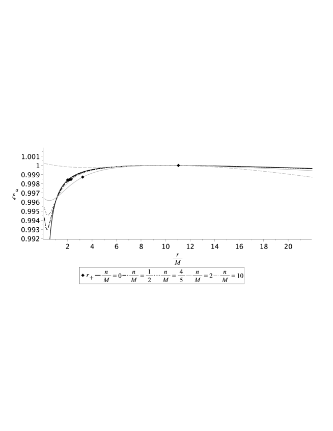
Since for $\delta_{1}=0$ the right sides of Eqs. (28) and (29) are trivial, and nonzero values of $\delta_{1}$ differ in sign, we represent in the Figs. 1 and 2 spatial component of tidal force with $\delta_{1}=1$. Note also that expression (28) is different from (16).

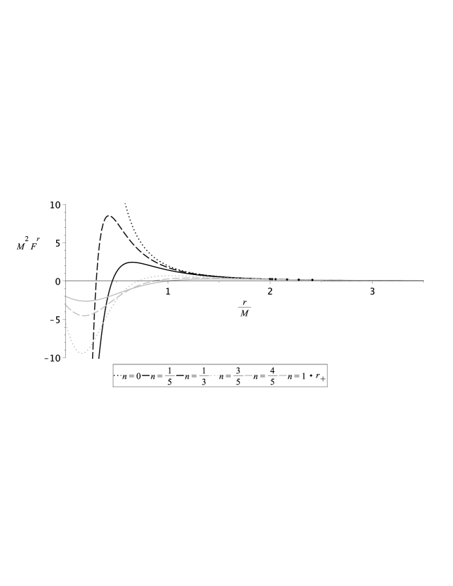
It is seen that at zero NUT-charge $n=0$ spatial components of tidal force has form

	$$\ddot{\xi}^{r}=\frac{2M\delta_{1}}{r^{3}}\xi^{r},$$		(30a)
	$$\ddot{\xi}^{a}=-\frac{M\delta_{1}}{r^{3}}\xi^{a},$$		(30b)

which are the same as the classic result from [32] for timelike geodesics with $\delta_{1}=1$. It should be noted that at a nonzero NUT-charge the investigated tidal forces do not become infinite at the point $r=0$. They are

	$$\ddot{\xi}^{r}\bigg{|}_{r=0}=-\frac{2\delta_{1}}{n^{2}}\xi^{r},$$		(31a)
	$$\ddot{\xi}^{a}\bigg{|}_{r=0}=\frac{\delta_{1}}{n^{2}}\xi^{a}.$$		(31b)

This is an important difference between the Taub–NUT spacetime and Schwarzschild spacetime, where all tidal force components have non-analytical behavior in $r=0$. However, their common feature is the regular behavior of tidal forces on the event horizon. Another important feature of the Taub–NUT metric is that the presence of the NUT-charge makes the spatial components of tidal forces alternating in sign, in contrast to the Schwarzschild metric, where all components were sign constant.

The points at which the tidal acceleration changes sign are determined by the equation

$$Mr^{3}+3n^{2}r^{2}-3Mn^{2}r-n^{4}=0$$

(32)

for all spatial components (28) and (29) of geodesic deviation vector. The roots of this equation define the points at which tidal stretching replaces tidal compression. The solution of this equation with respect to the variable $r$ is rather cumbersome, but we can see that the Eq.(32) is biquadratic with respect to the variable $n$. Therefore, we can explicitly express the NUT-charge

$$n^{2}=\frac{3}{2}\left(r^{2}-Mr\right)\left\{1+\sqrt{1+\frac{4Mr^{3}}{9\left(r^{2}-Mr\right)^{2}}}\right\},$$

(33)

where we dropped the root with minus before radical because the radical is greater than one, which makes the square of NUT-charge $n^{2}$ less than zero. Therefore solution (33) exists and is real at $r\geq M$.

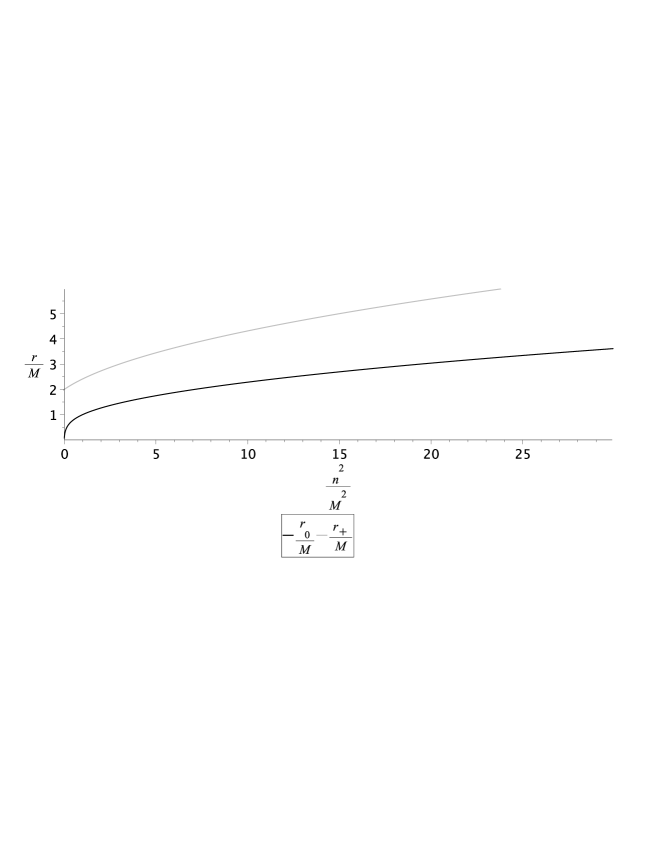
Fig. 3 shows inverse curve (33) and dependence of horizon radius (4) on $n^{2}$. It can be seen that the tidal acceleration zero point is below the event horizon at any values of NUT-charge $n$.

The extremum points of the curves shown in Figs. 1 and 2 are determined by the common equation

$$Mr^{4}+4n^{2}r^{3}-6Mn^{2}r^{2}-4n^{4}r+Mn^{4}=0.$$

(34)

It is an equation of the fourth degree with respect to $r$, but also biquadratic with respect to $n$. It allows us to express the charge in terms of the radial variable $r$

$$n^{2}=\frac{2r^{3}-3Mr^{2}}{4r-M}\left\{1\pm\sqrt{1+\frac{4Mr-M^{2}}{\left(2r-3M\right)^{2}}}\right\}.$$

(35)

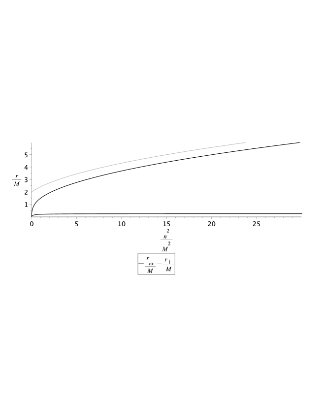
Fig. 4 shows inverse curve (35) and dependence of horizon radius (4) on $n^{2}$. It can be seen that the tidal acceleration extremum points is below the event horizon at any values of NUT-charge $n$.

It is also important to note that formulas (33)-(35) and Figs. 3 and 4 are valid for both the radial and angular components of tidal forces, because the right-hand sides of expressions (28) and (29) differ only by a factor, which does not affect the position of tidal equilibrium points and extrema of tidal acceleration.

In Eqs. (26) and (27) below, we pass from differentiation with respect to the affine parameter $\tau$ to differentiation with respect to the radial variable $r$ using Eq. (12). So they take the form

$$\left(E^{2}-\delta_{1}f\right){\xi^{r}}^{\prime\prime}-\frac{\delta_{1}f^{\prime}}{2}{\xi^{r}}^{\prime}+\frac{\delta_{1}f^{\prime\prime}}{2}\xi^{r}=0,$$

(36)

$$\left(E^{2}-\delta_{1}f\right){\xi^{a}}^{\prime\prime}-\frac{\delta_{1}f^{\prime}}{2}{\xi^{a}}^{\prime}+\left(\frac{\delta_{1}rf^{\prime}}{2\left(r^{2}+n^{2}\right)}+\frac{\delta_{1}n^{2}f}{\left(r^{2}+n^{2}\right)^{2}}\right)\xi^{a}=0,$$

(37)

where $a=\theta,\;\phi$. Solutions to these equations will be presented in the following sections.

For the convenience of further calculations, we pass to the dimensionless variables $\rho=\frac{r}{M}$ and $\nu=\frac{n}{M}$. These changes will allow us to eliminate the parameter $M$ from the Eqs. (36) and (37). Therefore, in all further considerations the prime will mean differentiation with respect to $\rho$ and in new terms function $f$ from (2) is

$$f(\rho)=1-\frac{2\rho+2\nu^{2}}{\rho^{2}+\nu^{2}}.$$

(38)

To compare the new solutions with the previously known ones, we present the solutions of the Eqs. (36) and (37) without NUT-charge, i.e. in Schwarzschild spacetime for $\nu=0$. Such solutions are expressed in terms of elementary functions

$$\xi^{r}=A\alpha(\rho)+\frac{B}{\psi^{4}}\left[6+\psi^{2}\rho+\frac{3\alpha(\rho)}{\psi}\ln\left(\frac{\alpha(\rho)-\psi}{\alpha(\rho)+\psi}\right)\right],$$

(39)

$$\xi^{a}=\rho\bigg{(}C+D\alpha(\rho)\bigg{)},$$

(40)

where

$$\psi=\sqrt{E^{2}-1},\;\alpha(\rho)=\sqrt{E^{2}-1+\frac{2}{\rho}},$$

(41)

and $A,B,C$ and $D$ are integration constants. These solutions were firstly obtained in Ref. [2]. In the vicinity of $\rho=0$ they are

	$$\xi^{r}(\rho)=\frac{A\sqrt{2}}{\sqrt{\rho}}+O\left(\sqrt{\rho}\right)\;\text{for}\;\rho\to 0,$$		(42a)
	$$\xi^{a}(\rho)=\sqrt{2}D\sqrt{\rho}+O\left(\rho\right)\;\text{for}\;\rho\to 0.$$		(42b)

The same solutions in the vicinity of $\rho=\infty$ behave

	$$\xi^{r}(\rho)=\frac{B}{E^{2}-1}\rho+O\left(1\right)\;\text{for}\;\rho\to\infty,$$		(43a)
	$$\xi^{a}(\rho)=\left(C+D\sqrt{E^{2}-1}\right)\rho+O\left(1\right)\;\text{for}\;\rho\to\infty.$$		(43b)

References

- [1] Schwarzschild K. Berliner Sitzungsbesichte (Phys. Math. Klasse), 189 – 196 3 Feb. (1916).
- [2] Fush H. Ann. Physik, 495, 231 – 233 (1983).
- [3] Reissner H. Ann. Physik, 50, 106 – 120 (1916).
- [4] Nordström G. Proc. Kon. Ned. Akad. Wet., 20, 1238 – 1245 (1918).
- [5] Kottler F. Ann. Physik, 56, 401 – 462 (1918).
- [6] Crispino L.C.B., et al.: Eur. Phys. J. C 76, 168 (2016).
- [7] Vandeev V.P., Semenova A.N.: Eur. Phys. J. C 81: 610 (2021).
- [8] Shahzad M. U., Jawad A., Eur. Phys. J. C 77, 372 (2017).
- [9] Kiselev, V. V.: Class. Quant. Grav. 20, 1187 (2003).
- [10] Luminet J. P., Marck J .A., Mon. Not. R. Astron. Soc. 212, 57 (1985).
- [11] B.P. Abbott, et al., LIGO Scientific, Virgo, Phys. Rev. Lett. 116 061102 (2016).
- [12] B.P. Abbott, et al., LIGO Scientific, VIRGO, Phys. Rev. Lett. 118 221101 (2017), erratum: Phys. Rev. Lett. 121 129901 (2018).
- [13] A. Goel, R. Maity, P. Roy, and T. Sarkar, Phys. Rev. D 91, 104029(2015)
- [14] Sharif M., Sadiq S., JETP 153, 232 – 239 (2018).
- [15] Haroldo C. D. Lima Junior, et al.: Int. J. Mod. Phys. D 29, 2041014 (2020)
- [16] Soon-Tae Hong, et al. Phys. Lett. B 881 135967 (2020).
- [17] Jing Li, et al. Eur. Phys. J. C 81, 590 (2021).
- [18] Siddharth Madan, Parth Bambhaniya, https://doi.org/10.48550/arXiv.2201.13163
- [19] Jiayi Liu, Songbai Chen, Jiliang Jing, https://doi.org/10.48550/arXiv.2203.14039
- [20] Kerr R. P. Phys. Rev. Lett., 11, 237 – 238 September 1. (1963).
- [21] E. Newman, L. Tamburino, and T. Unti, J. Math. Phys. 4, 915 (1963).
- [22] Newman E. T., Couch E., Chindapared K. et al. J. Math. Phys., 6, 918 – 919 (1965).
- [23] Haroldo C. D. Lima Junior, et al.: Eur. Phys. J. Plus 135: 334 (2020).
- [24] Chicone C., Mashhoon B., Punsly B., Int. J. Mod. Phys. D 13, 945 (2004).
- [25] Chicone C., Mashhoon B., Annalen Phys. 14, 290 (2005).
- [26] Bini D., Chicone C., Mashhoon B., Phys. Rev. D 95, 104029 (2017).
- [27] Shirokov M. F. Gen. Rel. Grav., 4, 131 (1973).
- [28] Nduka A. Gen. Rel. Grav., 8, 347 (1977).
- [29] Melkumova E.Yu., et al.: Sov. Phys. J., 33, 349 (1990).
- [30] B. Carter, Phys. Rev. 174, 1559 (1968).
- [31] Valeria Kagramanova, et al. Phys. Rev. D 81, 124044 (2010).
- [32] Misner C. W., Thorne K. S., Wheeler J. A., Gravitation (San Francisco: W.H. Freeman, 1973).