Geometric Inference on Kernel Density Estimates
We show that geometric inference of a point cloud can be calculated by examining its kernel density estimate with a Gaussian kernel. This allows one to consider kernel density estimates, which are robust to spatial noise, subsampling, and approximate computation in comparison to raw point sets. This is achieved by examining the sublevel sets of the kernel distance, which isomorphically map to superlevel sets of the kernel density estimate. We prove new properties about the kernel distance, demonstrating stability results and allowing it to inherit reconstruction results from recent advances in distance-based topological reconstruction. Moreover, we provide an algorithm to estimate its topology using weighted Vietoris-Rips complexes.
1 Introduction
Geometry and topology have become essential tools in modern data analysis: geometry to handle spatial noise and topology to identify the core structure. Topological data analysis (TDA) has found applications spanning protein structure analysis [32, 52] to heart modeling [41] to leaf science [60], and is the central tool of identifying quantities like connectedness, cyclic structure, and intersections at various scales. Yet it can suffer from spatial noise in data, particularly outliers.
When analyzing point cloud data, classically these approaches consider -shapes [31], where each point is replaced with a ball of radius , and the union of these balls is analyzed. More recently a distance function interpretation [11] has become more prevalent where the union of -radius balls can be replaced by the sublevel set (at value ) of the Hausdorff distance to the point set. Moreover, the theory can be extended to other distance functions to the point sets, including the distance-to-a-measure [15] which is more robust to noise.
This has more recently led to statistical analysis of TDA. These results show not only robustness in the function reconstruction, but also in the topology it implies about the underlying dataset. This work often operates on persistence diagrams which summarize the persistence (difference in function values between appearance and disappearance) of all homological features in single diagram. A variety of work has developed metrics on these diagrams and probability distributions over them [55, 67], and robustness and confidence intervals on their landscapes [7, 39, 18] (summarizing again the most dominant persistent features [19]). Much of this work is independent of the function and data from which the diagram is generated, but it is now more clear than ever, it is most appropriate when the underlying function is robust to noise, e.g., the distance-to-a-measure [15].
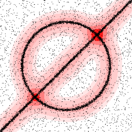
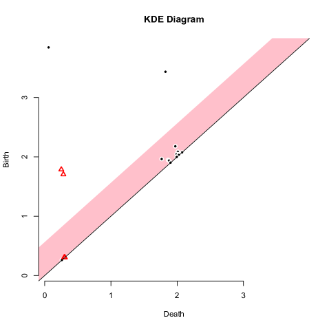
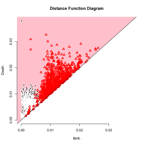
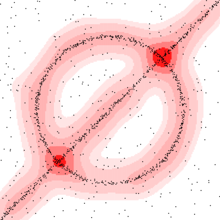
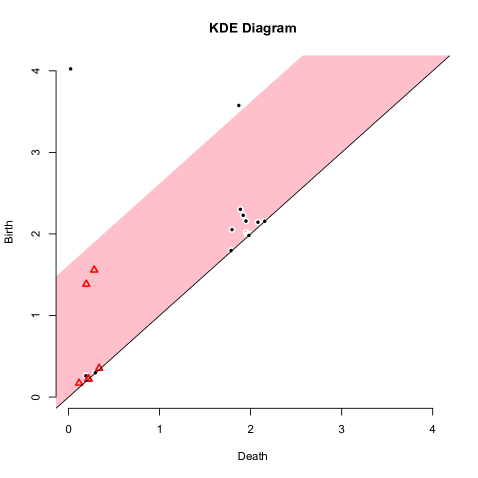
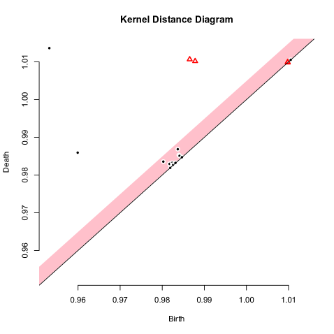
A very recent addition to this progression is the new TDA package for R [38]; it includes built in functions to analyze point sets using Hausdorff distance, distance-to-a-measure, -nearest neighbor density estimators, kernel density estimates, and kernel distance. The example in Figure 1 used this package to generate persistence diagrams. While, the stability of the Hausdorff distance is classic [11, 31], and the distance-to-a-measure [15] and -nearest neighbor distances have been shown robust to various degrees [5], this paper is the first to analyze the stability of kernel density estimates and the kernel distance in the context of geometric inference. Some recent manuscripts show related results. Bobrowski et al. [6] consider kernels with finite support, and describe approximate confidence intervals on the superlevel sets, which recover approximate persistence diagrams. Chazal et al. [17] explore the robustness of the kernel distance in bootstrapping-based analysis.
In particular, we show that the kernel distance and kernel density estimates, using the Gaussian kernel, inherit some reconstruction properties of distance-to-a-measure, that these functions can also be approximately reconstructed using weighted (Vietoris-)Rips complexes [8], and that under certain regimes can infer homotopy of compact sets. Moreover, we show further robustness advantages of the kernel distance and kernel density estimates, including that they possess small coresets [57, 71] for persistence diagrams and inference.
1.1 Kernels, Kernel Density Estimates, and Kernel Distance
A kernel is a non-negative similarity measure ; more similar points have higher value. For any fixed , a kernel can be normalized to be a probability distribution; that is . For the purposes of this article we focus on the Gaussian kernel defined as . 111 is normalized so that for . The choice of coefficient is not the standard normalization, but it is perfectly valid as it scales everything by a constant. It has the property that for small.
A kernel density estimate [65, 61, 26, 27] is a way to estimate a continuous distribution function over for a finite point set ; they have been studied and applied in a variety of contexts, for instance, under subsampling [57, 71, 3], motion planning [59], multimodality [64, 33], and surveillance [37], road reconstruction [4]. Specifically,
The kernel distance [47, 42, 48, 58] (also called current distance or maximum mean discrepancy) is a metric [56, 66] between two point sets , (as long as the kernel used is characteristic [66], a slight restriction of being positive definite [2, 70], this includes the Gaussian and Laplace kernels). Define a similarity between the two point sets as
Then the kernel distance between two point sets is defined as
When we let point set be a single point , then .
Kernel density estimates can apply to any measure (on ) as The similarity between two measures is where is the product measure of and (), and then the kernel distance between two measures and is still a metric, defined as When the measure is a Dirac measure at ( for , but integrates to ), then . Given a finite point set , we can work with the empirical measure defined as , where is the Dirac measure on , and .
If is positive definite, it is said to have the reproducing property [2, 70]. This implies that is an inner product in some reproducing kernel Hilbert space (RKHS) . Specifically, there is a lifting map so that , and moreover the entire set can be represented as , which is a single element of and has a norm . A single point also has a norm in this space.
1.2 Geometric Inference and Distance to a Measure: A Review
Given an unknown compact set and a finite point cloud that comes from under some process, geometric inference aims to recover topological and geometric properties of from . The offset-based (and more generally, the distance function-based) approach for geometric inference reconstructs a geometric and topological approximation of by offsets from (e.g. [13, 14, 15, 20, 21]).
Given a compact set , we can define a distance function to ; a common example is (i.e. -shapes). The offsets of are the sublevel sets of , denoted . Now an approximation of by another compact set (e.g. a finite point cloud) can be quantified by the Hausdorff distance of their distance functions. The intuition behind the inference of topology is that if is small, thus and are close, and subsequently, , and carry the same topology for an appropriate scale . In other words, to compare the topology of offsets and , we require Hausdorff stability with respect to their distance functions and . An example of an offset-based topological inference result is formally stated as follows (as a particular version of the reconstruction Theorem 4.6 in [14]), where the reach of a compact set , , is defined as the minimum distance between and its medial axis [54].
Theorem 1.1 (Reconstruction from [14]).
Let be compact sets such that and . Then and are homotopy equivalent for sufficiently small (e.g., ) if .
Here ensures that the topological properties of and are the same, and the parameter ensures and are close. Typically is tied to the density with which a point cloud is sampled from .
For function to be distance-like it should satisfy the following properties:
-
•
(D1) is -Lipschitz: For all , .
-
•
(D2) is -semiconcave: The map is concave.
-
•
(D3) is proper: tends to the infimum of its domain (e.g., ) as tends to infinity.
In addition to the Hausdorff stability property stated above, as explained in [15], is distance-like. These three properties are paramount for geometric inference (e.g. [14, 53]). (D1) ensures that is differentiable almost everywhere and the medial axis of has zero -volume [15]; and (D2) is a crucial technical tool, e.g., in proving the existence of the flow of the gradient of the distance function for topological inference [14].
Distance to a measure.
Given a probability measure on and a parameter smaller than the total mass of , the distance to a measure [15] is defined for any point as
It has been shown in [15] that is a distance-like function (satisfying (D1), (D2), and (D3)), and:
-
•
(M4) [Stability] For probability measures and on and , then .
Here is the Wasserstein distance [69]: between two measures, where measures the amount of mass transferred from location to location and is a transference plan [69].
1.3 Our Results
We show how to estimate the topology (e.g., approximate persistence diagrams, infer homotopy of compact sets) using superlevel sets of the kernel density estimate of a point set . We accomplish this by showing that a similar set of properties hold for the kernel distance with respect to a measure , (in place of distance to a measure ), defined as
This treats as a probability measure represented by a Dirac mass at . Specifically, we show is distance-like (it satisfies (D1), (D2), and (D3)), so it inherits reconstruction properties of . Moreover, it is stable with respect to the kernel distance:
-
•
(K4) [Stability] If and are two measures on , then .
In addition, we show how to construct these topological estimates for using weighted Rips complexes, following power distance machinery introduced in [8]. That is, a particular form of power distance permits a multiplicative approximation with the kernel distance.
We also describe further advantages of the kernel distance. (i) Its sublevel sets conveniently map to the superlevel sets of a kernel density estimate. (ii) It is Lipschitz with respect to the smoothing parameter when the input is fixed. (iii) As tends to for any two probability measures , the kernel distance is bounded by the Wasserstein distance: . (iv) It has a small coreset representation, which allows for sparse representation and efficient, scalable computation. In particular, an -kernel sample [48, 57, 71] of is a finite point set whose size only depends on and such that . These coresets preserve inference results and persistence diagrams.
2 Kernel Distance is Distance-Like
In this section we prove satisfies (D1), (D2), and (D3); hence it is distance-like. Recall we use the -normalized Gaussian kernel . For ease of exposition, unless otherwise noted, we will assume is fixed and write instead of .
2.1 Semiconcave Property for
Lemma 2.1 (D2).
is -semiconcave: the map is concave.
Proof 2.2.
Let . The proof will show that the second derivative of along any direction is nonpositive. We can rewrite
Note that both and are absolute constants, so we can ignore them in the second derivative. Furthermore, by setting , the second derivative of is nonpositive if the second derivative of is nonpositive for all . First note that the second derivative of is a constant in every direction. The second derivative of is symmetric about , so we can consider the second derivative along any vector ,
This reaches its maximum value at where it is ; this follows setting the derivative of to , (), substituting .
We also note in Appendix A that semiconcavity follows trivially in the RKHS .
2.2 Lipschitz Property for
We generalize a (folklore, see [15]) relation between semiconcave and Lipschitz functions and prove it for completeness. A function is -semiconcave if the function is concave.
Lemma 2.3.
Consider a twice-differentiable function and a parameter . If is -semiconcave, then is -Lipschitz.
Proof 2.4.
The proof is by contrapositive; we assume that is not -Lipschitz and then show cannot be -semiconcave. By this assumption, then in some direction , there is a point such that .
Now we examine at , and specifically its second derivative in direction .
Since , then and is not -semiconcave at .
Lemma 2.5 (D1).
is -Lipschitz on its input.
2.3 Properness of
Finally, for to be distance-like, we need to show it is proper when its range is restricted to be less than . Here, the value of depends on not on since . This is required for a distance-like version [15], Proposition 4.2) of the Isotopy Lemma ([44], Proposition 1.8).
Lemma 2.6 (D3).
is proper.
We delay this technical proof to Appendix A. The main technical difficulty comes in mapping standard definitions and approaches for distance functions to our function with a restricted range.
Also by properness (see discussion in Appendix A), Lemma 2.6 also implies that is a closed map and its levelset at any value is compact. This also means that the sublevel set of (for ranges ) is compact. Since the levelset (sublevel set) of corresponds to the levelset (superlevel set) of , we have the following corollary.
Corollary 2.7.
The superlevel sets of for all ranges with threshold , are compact.
The result in [33] shows that given a measure defined by a point set of size , the has polynomial in modes; hence the superlevel sets of are compact in this setting. The above corollary is a more general statement as it holds for any measure.
3 Power Distance using Kernel Distance
A power distance using is defined with a point set and a metric on ,
A point takes the distance under to the closest , plus a weight from ; thus a sublevel set of is defined by a union of balls. We consider a particular choice of the distance which leads to a kernel version of power distance
In Section 4.2 we use to adapt the construction introduced in [8] to approximate the persistence diagram of the sublevel sets of , using a weighted Rips filtration of .
Given a measure , let , and let be a point set that contains . We show below, in Theorem 3.8 and Theorem 3.2, that . However, constructing exactly seems quite difficult. We also attempt to use in place of (see Section C.1), but are not able to obtain useful bounds.
Now consider an empirical measure defined by a point set . We show (in Theorem C.21 in Appendix C.2) how to construct a point (that approximates ) such that for any . For a point set , the median concentration is a radius such that no point has more than half of the points of within , and the spread is the ratio between the longest and shortest pairwise distances. The runtime is polynomial in and assuming is bounded, and that and are constants.
Then we consider , where is found with in the above construction. Then we can provide the following multiplicative bound, proven in Theorem 3.10. The lower bound holds independent of the choice of as shown in Theorem 3.2.
Theorem 3.1.
For any point set and point , with empirical measure defined by , then
3.1 Kernel Power Distance for a Measure
First consider the case for a kernel power distance where is an arbitrary measure.
Theorem 3.2.
For measure , point set , and ,
Proof 3.3.
Let . Then we can use the triangle inequality and to show
Lemma 3.4.
For measure , point set , point , and point then
Proof 3.5.
Again, we can reach this result with the triangle inequality.
Recall the definition of a point .
Lemma 3.6.
For any measure and point we have .
Proof 3.7.
Since is a point in , and thus . Then by triangle inequality of to see that .
Theorem 3.8.
For any measure in and any point , using the point then .
We now need two properties of the point set to reach our bound, namely, the spread and the median concentration . Typically is not too large, and it makes sense to choose so , or at least .
Theorem 3.10.
Consider any point set of size , with measure , spread , and median concentration . We can construct a point set in time such that for any point ,
4 Reconstruction and Topological Estimation using Kernel Distance
Now applying distance-like properties from Section 2 and the power distance properties of Section 3 we can apply known reconstruction results to the kernel distance.
4.1 Homotopy Equivalent Reconstruction using
We have shown that the kernel distance function is a distance-like function. Therefore the reconstruction theory for a distance-like function [15] (which is an extension of results for compact sets [14]) holds in the setting of . We state the following two corollaries for completeness, whose proofs follow from the proofs of Proposition 4.2 and Theorem 4.6 in [15]. Before their formal statement, we need some notation adapted from [15] to make these statements precise. Let be a distance-like function. A point is an -critical point if with , . Let denote the sublevel set of , and let denote all points at levels in the range . For , the -reach of is the maximum such that has no -critical point, denoted as . When , coincides with reach introduced in [40].
Theorem 4.1 (Isotopy lemma on ).
Let be two positive numbers such that has no critical points in . Then all the sublevel sets are isotopic for .
Theorem 4.2 (Reconstruction on ).
Let and be two kernel distance functions such that . Suppose for some . Then , and , the sublevel sets and are homotopy equivalent for .
4.2 Constructing Topological Estimates using
In order to actually construct a topological estimate using the kernel distance , one needs to be able to compute quantities related to its sublevel sets, in particular, to compute the persistence diagram of the sub-level sets filtration of . Now we describe such tools needed for the kernel distance based on machinery recently developed by Buchet et al. [8], which shows how to approximate the persistent homology of distance-to-a-measure for any metric space via a power distance construction. Then using similar constructions, we can use the weighted Rips filtration to approximate the persistence diagram of the kernel distance.
To state our results, first we require some technical notions and assume basic knowledge on persistent homology (see [34, 35] for a readable background). Given a metric space with the distance , a set and a function , the (general) power distance associated with is defined as Now given the set and its corresponding power distance , one could use the weighted Rips filtration to approximate the persistence diagram of , under certain restrictive conditions proven in Appendix D.1. Consider the sublevel set of , . It is the union of balls centered at points with radius for each . The weighted Čech complex for parameter is the union of simplices such that . The weighted Rips complex for parameter is the maximal complex whose -skeleton is the same as . The corresponding weighted Rips filtration is denoted as .
Setting and given point set described in Section 3, consider the weighted Rips filtration based on the kernel power distance, . We view the persistence diagrams on a logarithmic scale, that is, we change coordinates of points following the mapping . denotes the corresponding bottleneck distance between persistence diagrams. We now state a corollary of Theorem 3.1.
Corollary 4.3.
The weighted Rips filtration can be used to approximate the persistence diagram of such that .
Proof 4.4.
To prove that two persistence diagrams are close, one could prove that their filtration are interleaved [12], that is, two filtrations and are -interleaved if for any , .
First, Lemmas D.1 and D.3 prove that the persistence diagrams and are well-defined. Second, the results of Theorem 3.1 implies an multiplicative interleaving. Therefore for any ,
On a logarithmic scale (by taking the natural log of both sides), such interleaving becomes addictive,
Theorem 4 of [16] implies
In addition, by the Persistent Nerve Lemma ([22], Theorem 6 of [62], an extension of the Nerve Theorem [46]), the sublevel sets filtration of , which correspond to unions of balls of increasing radius, has the same persistent homology as the nerve filtration of these balls (which, by definition, is the Čech filtration). Finally, there exists a multiplicative interleaving between weighted Rips and Čech complexes (Proposition 31 of [16]), We then obtain the following bounds on persistence diagrams,
We use triangle inequality to obtain the final result:
Based on Corollary 4.3, we have an algorithm that approximates the persistent homology of the sublevel set filtration of by constructing the weighted Rips filtration corresponding to the kernel-based power distance and computing its persistent homology. For memory efficient computation, sparse (weighted) Rips filtrations could be adapted by considering simplices on subsamples at each scale [63, 16], although some restrictions on the space apply.
4.3 Distance to the Support of a Measure vs. Kernel Distance
Suppose is a uniform measure on a compact set in . We now compare the kernel distance with the distance function to the support of . We show how approximates , and thus allows one to infer geometric properties of from samples from .
A generalized gradient and its corresponding flow associated with a distance function are described in [14] and later adapted for distance-like functions in [15]. Let be a distance function associated with a compact set of . It is not differentiable on the medial axis of . A generalized gradient function coincides with the usual gradient of where is differentiable, and is defined everywhere and can be integrated into a continuous flow that points away from . Let be an integral (flow) line. The following lemma shows that when close enough to , that is strictly increasing along any . The proof is quite technical and is thus deferred to Appendix D.2.
Lemma 4.5.
Given any flow line associated with the generalized gradient function , is strictly monotonically increasing along for sufficiently far away from the medial axis of , for and . Here denotes a ball of radius , , and suppose .
The strict monotonicity of along the flow line under the conditions in Lemma 4.5 makes it possible to define a deformation retract of the sublevel sets of onto sublevel sets of . Such a deformation retract defines a special case of homotopy equivalence between the sublevel sets of and sublevel sets of . Consider a sufficiently large point set sampled from , and its induced measure . We can then also invoke Theorem 4.2 and a sampling bound (see Section 6 and Lemma B.3) to show homotopy equivalence between the sublevel sets of and .
5 Stability Properties for the Kernel Distance to a Measure
Lemma 5.1 (K4).
For two measures and on we have .
Proof 5.2.
Since is a metric, then by triangle inequality, for any we have and . Therefore for any we have , proving the claim.
Both the Wasserstein and kernel distance are integral probability metrics [66], so (M4) and (K4) are both interesting, but not easily comparable. We now attempt to reconcile this.
5.1 Comparing to
Lemma 5.3.
There is no Lipschitz constant such that for any two probability measures and we have .
Proof 5.4.
Consider two measures and which are almost identical: the only difference is some mass of measure is moved from its location in a distance in . The Wasserstein distance requires a transportation plan that moves this mass in back to where it was in with cost in . On the other hand, is bounded.
We conjecture for any two probability measures and that . This would show that is at least as stable as since a bound on would also bound , but not vice versa. Alternatively, this can be viewed as is less discriminative than ; we view this as a positive in this setting, as it is mainly less discriminative towards outliers (far away points). Here we only show that this property for a special case and as . To simplify notation, all integrals are assumed to be over the full domain .
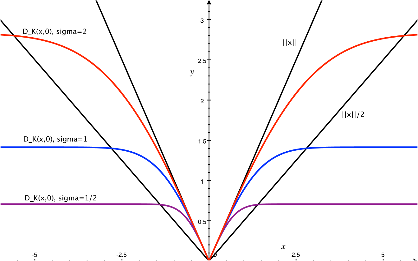
Two Dirac masses.
We first consider a special case when is a Dirac mass at a point and is a Dirac mass at a point . That is they are both single points. We can then write . Figure 2 illustrates the result of this lemma.
Lemma 5.5.
For any points it always holds that . When then .
Proof 5.6.
First expand as
Now using that for
and
where the last inequality holds when .
One Dirac mass.
Consider the case where one measure is a Dirac mass at point .
Lemma 5.7.
Consider two probability measures and on where is represented by a Dirac mass at a point . Then for any , where the equality only holds when is also a Dirac mass at .
Proof 5.8.
Since both and are metrics and hence non-negative, we can instead consider their squared versions: and
Now use the bound for to approximate
The inequality becomes an equality only when for all , and since they are both metrics, this is the only location where they are both .
General case.
Next we show that if is not a unit Dirac, then this inequality holds in the limit as goes to infinity. The technical work is making precise how and how this compares to bounds on and .
For simpler exposition, we assume is a probability measure, that is ; otherwise we can normalize at the appropriate locations, and all of the results go through.
Lemma 5.9.
For any we have
Proof 5.10.
We use the Taylor expansion of . Then it is easy to see
This lemma illustrates why the choice of coefficient of is convenient. Since then acts like , and becomes closer as increases. Define to represent the mean point of measure ; to represent the variance of the measure ; and .
Lemma 5.11.
For any we have
Proof 5.12.
Lemma 5.13.
For probability measures and on ,
Proof 5.14.
Theorem 5.15.
For any two probability measures and defined on
Proof 5.16.
First expand
Finally we observe that since all terms of are divided by or larger powers of . Thus as increases approaches and approaches , completing the proof.
Now we can relate to through . The next result is a known lower bounds for the Earth movers distance [23][Theorem 7]. We reprove it in Appendix E for completeness.
Lemma 5.17.
For any probability measures and defined on we have
We can now combine these results to achieve the following theorem.
Theorem 5.18.
For any two probability measures and defined on and Thus .
5.2 Kernel Distance Stability with Respect to
We now explore the Lipschitz properties of with respect to the noise parameter . We argue any distance function that is robust to noise needs some parameter to address how many outliers to ignore or how far away a point is that is an outlier. For instance, this parameter in is which controls the amount of measure to be used in the distance.
Here we show that has a particularly nice property, that it is Lipschitz with respect to the choice of for any fixed . The larger the more effect outliers have, and the smaller the less the data is smoothed and thus the closer the noise needs to be to the underlying object to effect the inference.
Lemma 5.19.
Let . We can bound , and over any choice of .
Proof 5.20.
The first bound follows from and for .
Next we define
Now to solve the first part, we differentiate with respect to to find its maximum over all choices of .
Where at , and as approaches . Thus the maximum must occur at one of these values. Both and , while , proving the first part.
To solve the second part, we perform the same approach on .
Thus at and as goes to for . Both and . The minimum occurs at . The maximum occurs at .
Theorem 5.21.
For any measure defined on and , is -Lipschitz with respect to , for .
Proof 5.22.
Recall that is the product measure of any and , and define as . It is now useful to define a function as
So and we can write another function as
Now to prove is -Lipschitz, we can show that is -semiconcave with respect to , and apply Lemma 2.3. This boils down to showing the second derivative of is always non-positive.
First we note that since for any product distribution of two distributions and , including when or is a Dirac mass, then
Thus since is in for all choices of , , and , then and . This bounds the third term in , we now need to use a similar approach to bound the first and second terms.
Let , so we can apply Lemma 5.19.
Then we complete the proof using the upper bound of each item of
Lipschitz in for .
We show that there is no Lipschitz property for , with respect to that is independent of the measure . Consider a measure for point set consisting of two points at and at . Now consider . When then is constant. But for for , then and , which is maximized as approaches with an infimum of . If points are at and point at , then the infimum of the first derivative of is . Hence for a measure defined by a point set, the infimum of and, hence a lower bound on the Lipschitz constant is where .
6 Algorithmic and Approximation Observations
Kernel coresets.
The kernel distance is robust under random samples [48]. Specifically, if is a point set randomly chosen from of size then with probability at least . We call such a subset and -kernel sample of . Furthermore, it is also possible to construct -kernel samples with even smaller size of [57]; in particular in the required size is . Exploiting the above constructions, recent work [71] builds a data structure to allow for efficient approximate evaluations of where .
These constructions of also immediately imply that since , and both the first and third term incur at most error in converting to and , respectively (see Lemma B.1). Thus, an -kernel sample of implies that (see Lemma B.3).
This implies algorithms for geometric inference on enormous noisy data sets. Moreover, if we assume an input point set is drawn iid from some underlying, but unknown distribution , we can bound approximations with respect to .
Corollary 6.1.
Consider a measure defined on , a kernel , and a parameter . We can create a coreset of size or randomly sample points so, with probability at least , any sublevel set is homotopy equivalent to for and .
Stability of persistence diagrams.
Furthermore, the stability results on persistence diagrams [24] hold for kernel density estimates and kernel distance of and (where is a coreset of with the same size bounds as above). If , then , where is the bottleneck distance between persistence diagrams. Combined with the coreset results above, this immediately implies the following corollaries.
Corollary 6.3.
Consider a measure defined on and a kernel . We can create a core set of size or randomly sample points which will have the following properties with probability at least .
-
•
.
-
•
.
Corollary 6.4.
Consider a measure defined on and a kernel . We can create a coreset of size or randomly sample points which will have the following property with probability at least .
-
•
.
Another bound was independently derived to show an upper bound on the size of a random sample such that in [3]; this can, as above, also be translated into bounds for and . This result assumes and is parametrized by a bandwidth parameter that retains that for all using that and . This ensures that is -Lipschitz and that for any . Then their bound requires random samples.
To compare directly against the random sampling result we derive from Joshi et al. [48], for kernel then . Hence, our analysis requires , and is an improvement when or is not known or bounded, as well as in some other cases as a function of , , , and .
7 Discussion
We mention here a few other interesting aspects of our results and observations about topological inference using the kernel distance. They are related to how the noise parameter affects the idea of scale, and a few more experiments, including with alternate kernels.
7.1 Noise and Scale
Much of geometric and topological reconstruction grew out of the desire to understand shapes at various scales. A common mechanism is offset based; e.g., -shapes [31] represent the scale of a shape with the parameter controlling the offsets of a point cloud. There are two parameters with the kernel distance: controls the offset through the sublevel set of the function, and controls the noise. We argue that any function which is robust to noise must have a parameter that controls the noise (e.g. for and for ). Here clearly defines some sense of scale in the setting of density estimation [65] and has a geometrical interpretation, while represents a fraction of the measure and is hard to interpret geometrically, as illustrated by the lack of a Lipschitz property for with respect to .
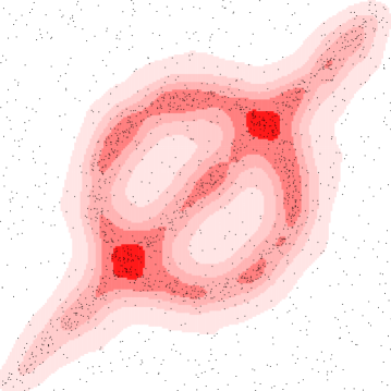
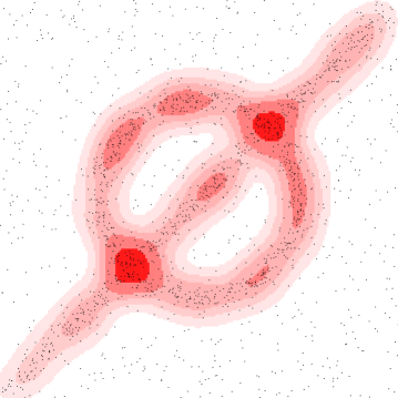
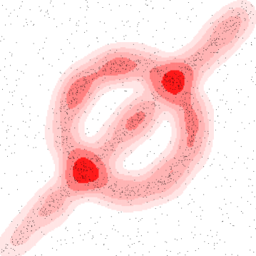
There are several experiments below, in Section 7.2, from which several insights can be drawn. One observation is that even though there are two parameters and that control the scale, the interesting values typically have very close to . Thus, we recommend to first set to control the scale at which the data is studied, and then explore the effect of varying for values near . Moreover, not much structure seems to be missed by not exploring the space of both parameters; Figure 3 shows that fixing one (of and ) and varying the other can provide very similar superlevel sets. However, it is possible instead to fix and explore the persistent topological features in the data [36, 34] (those less affected by smoothing) by varying . On the other hand, it remains a challenging problem to study two parameter persistent homology [10, 9] under the setting of kernel distance (or kernel density estimate).
7.2 Experiments
We consider measures defined by a point set . To experimentally visualize the structures of the superlevel sets of kernel density estimates, or equivalently sublevel sets of the kernel distance, we do the simplest thing and just evaluate at every grid point on a sufficiently dense grid.
Grid approximation.
Due to the -Lipschitz property of the kernel distance, well chosen grid points have several nice properties. We consider the functions up to some resolution parameter , consistent with the parameter used to create a coreset approximation . Now specifically, consider an axis-aligned grid with edge length so no point is further than from some grid point . Since when , we only need to consider grid points which are within of some point (or , of coreset of ) [48, 71]. This is at most grid points total for a fixed constant. Furthermore, due to the -Lipschitz property of , when considering a specific level set at
-
•
a point such that is no further than from some such that , and
-
•
every ball centered at some point of radius so that all has has some representative point such that , and hence .
Thus “deep” regions and spatially thick features are preserved, however thin passageways or layers that are near the threshold , even if they do not correspond to a critical point, may erroneously become disconnected, causing phantom components or other topological features. However, due to the Lipschitz property, these can be different from by at most , so the errors will have small deviation in persistence.
Varying parameter or .
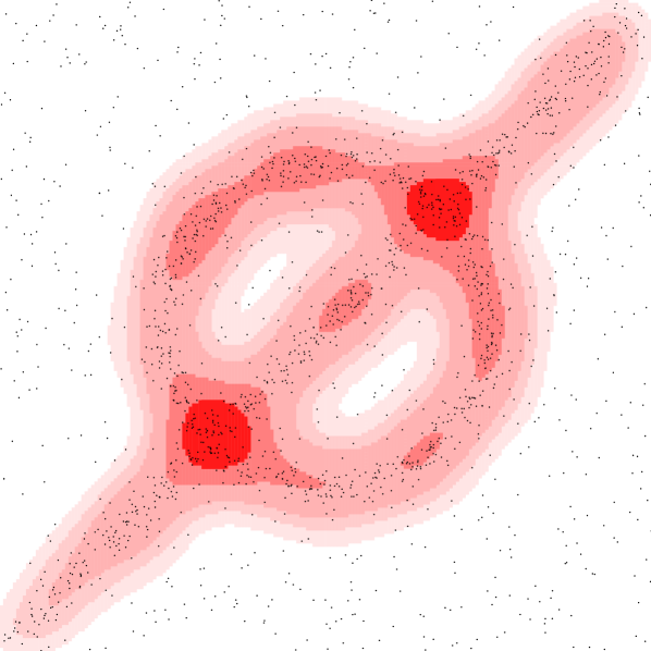
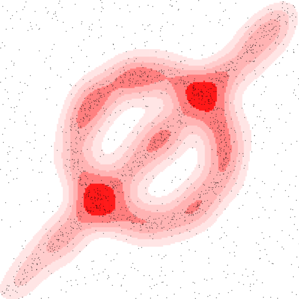
We demonstrate the geometric inference on a synthetic dataset in where points are chosen near a circle centered at with radius or along a line segment from to . Each point has Gaussian noise added with standard deviation . The remaining points are chosen uniformly from . We use a Gaussian kernel with . Figure 3 shows (left) various sublevel sets for the kernel distance at a fixed and (right) various superlevel sets for a fixed , but various values of , where
This choice of and were made to highlight how similar the isolevels can be.

Alternative kernels.
We can choose kernels other than the Gaussian kernel in the kernel density estimate, for instance
-
•
the Laplace kernel ,
-
•
the triangle kernel ,
-
•
the Epanechnikov kernel , or
-
•
the ball kernel (.
Figure 4 chooses parameters to make them comparable to the Figure 3(left). Of these only the Laplace kernel is characteristic [66] making the corresponding version of the kernel distance a metric. Investigating which of the above reconstruction theorems hold when using the Laplace or other kernels is an interesting question for future work.
Additionally, normal vector information and even -forms can be used in the definition of a kernel [42, 68, 30, 29, 43, 48]; this variant is known as the current distance. In some cases it retains its metric properties and has been shown to be very useful for shape alignment in conjunction with medical imaging.
7.3 Open Questions
This work shows it is possible to prove formal reconstruction results using kernel density estimates and the kernel distance. But it also opens many interesting questions.
-
•
For what other types of kernels can we show reconstruction bounds? The Laplace and triangle kernels are natural choices. For both the coresets results match those of the Gaussian kernel. The kernel distance under the Laplace kernel is also a metric, but is not known to be for the triangle kernel. Yet, the triangle kernel would be interesting since it has bounded support, and may lend itself to easier computation.
-
•
The power distance construction in Section 3 requires a point , which approximates the point with minimum kernel distance. This is intuitively because it is possible to construct a point set (say points lying on a circle with no points inside) such that the point which minimizes the kernel distance and maximizes the kernel density estimate is far from any point in the point set. For one, can be constructed efficiently without dependence on or ?
But more interestingly, can we generally approximate the persistence diagram without creating a simplicial complex on a subset of the input points? We do describe some bounds on using a grid-based technique in Section 7.2, but this is also unsatisfying since it essentially requires a low-dimensional Euclidean space.
-
•
Since is Lipschitz in and , it may make sense to understand the simultaneous stability of both variables. What is the best way to understand persistence over both parameters?
-
•
We provided some initial bound comparing the kernel distance under the Gaussian kernel and the Wasserstein distance. Can we show that under our choice of normalization that , unconstrained? More generally, how does the kernel distance under other kernels compare with other forms of Wasserstein and other distances on measures?
Acknowledgements
The authors thank Don Sheehy, Frédéric Chazal and the rest of the Geometrica group at INRIA-Saclay for enlightening discussions on geometric and topological reconstruction. We also thank Don Sheehy for personal communications regarding the power distance constructions, and Yusu Wang for ideas towards Lemma 4.5. Finally, we are also indebted to the anonymous reviewers for many detailed suggestions leading to improvements in results and presentation.
References
- [1] Pankaj K. Agarwal, Sariel Har-Peled, Hiam Kaplan, and Micha Sharir. Union of random minkowski sums and network vulnerability analysis. In Proceedings of 29th Symposium on Computational Geometry, 2013.
- [2] N. Aronszajn. Theory of reproducing kernels. Transactions of the American Mathematical Society, 68:337–404, 1950.
- [3] Sivaraman Balakrishnan, Brittany Terese Fasy, Fabrizio Lecci, Alessandro Rinaldo, Aarti Singh, and Larry Wasserman. Statistical inference for persistent homology. Technical report, ArXiv:1303.7117, March 2013.
- [4] James Biagioni and Jakob Eriksson. Map inference in the face of noise and disparity. In ACM SIGSPATIAL GIS, 2012.
- [5] Gérard Biau, Frédéric Chazal, David Cohen-Steiner, Luc Devroye, and Carlos Rodriguez. A weighted -nearest neighbor density estimate for geometric inference. Electronic Journal of Statistics, 5:204–237, 2011.
- [6] Omer Bobrowski, Sayan Mukherjee, and Jonathan E. Taylor. Topological consistency via kernel estimation. Technical report, arXiv:1407.5272, 2014.
- [7] Peter Bubenik. Statistical topological data analysis using persistence landscapes. Jounral of Machine Learning Research, 2014.
- [8] Mickael Buchet, Frederic Chazal, Steve Y. Oudot, and Donald R. Sheehy. Efficient and robust topological data analysis on metric spaces. arXiv:1306.0039, 2013.
- [9] Gunnar Carlsson, Gurjeet Singh, and Afra Zomorodian. Computing multidimensional persistence. Algorithms and Computation: Lecture Notes in Computer Science, 5878:730–739, 2009.
- [10] Gunnar Carlsson and Afra Zomorodian. The theory of multidimensional persistence. Proc. 23rd Ann. Symp. Computational Geometry, pages 184–193, 2007.
- [11] Frédéric Chazal and David Cohen-Steiner. Geometric inference. Tessellations in the Sciences, 2012.
- [12] Frédéric Chazal, David Cohen-Steiner, Marc Glisse, Leonidas J. Guibas, and Steve Y. Oudot. Proximity of persistence modules and their diagrams. In Proceedings 25th Annual Symposium on Computational Geometry, pages 237–246, 2009.
- [13] Frédéric Chazal, David Cohen-Steiner, and André Lieutier. Normal cone approximation and offset shape isotopy. Computational Geometry: Theory and Applications, 42:566–581, 2009.
- [14] Frédéric Chazal, David Cohen-Steiner, and André Lieutier. A sampling theory for compact sets in Euclidean space. Discrete Computational Geometry, 41(3):461–479, 2009.
- [15] Frédéric Chazal, David Cohen-Steiner, and Quentin Mérigot. Geometric inference for probability measures. Foundations of Computational Mathematics, 11(6):733–751, 2011.
- [16] Frederic Chazal, Vin de Silva, Marc Glisse, and Steve Oudot. The structure and stability of persistence modules. arXiv:1207.3674, 2013.
- [17] Frédéric Chazal, Brittany Terese Fasy, Fabrizio Lecci, Bertrand Michel, Alessandro Rinaldo, and Larry Wasserman. Robust topolical inference: Distance-to-a-measure and kernel distance. Technical report, arXiv:1412.7197, 2014.
- [18] Frédéric Chazal, Brittany Terese Fasy, Fabrizio Lecci, Alessandro Rinaldo, Aarti Singh, and Larry Wasserman. On the bootstrap for persistence diagrams and landscapes. Modeling and Analysis of Information Systems, 20:96–105, 2013.
- [19] Frédéric Chazal, Brittany Terese Fasy, Fabrizio Lecci, Alessandro Rinaldo, and Larry Wasserman. Stochastic convergence of persistence landscapes. In Proceedings Symposium on Computational Geometry, 2014.
- [20] Frédéric Chazal and André Lieutier. Weak feature size and persistent homology: computing homology of solids in rn from noisy data samples. Proceedings 21st Annual Symposium on Computational Geometry, pages 255–262, 2005.
- [21] Frédéric Chazal and André Lieutier. Topology guaranteeing manifold reconstruction using distance function to noisy data. Proceedings 22nd Annual Symposium on Computational Geometry, pages 112–118, 2006.
- [22] Frédéric Chazal and Steve Oudot. Towards persistence-based reconstruction in euclidean spaces. Proceedings 24th Annual Symposium on Computational Geometry, pages 232–241, 2008.
- [23] Scott Cohen. Finding color and shape patterns in images. Technical report, Stanford University: CS-TR-99-1620, 1999.
- [24] David Cohen-Steiner, Herbert Edelsbrunner, and John Harer. Stability of persistence diagrams. Discrete and Computational Geometry, 37:103–120, 2007.
- [25] Hal Daumé. From zero to reproducing kernel hilbert spaces in twelve pages or less. http://pub.hal3.name/daume04rkhs.ps, 2004.
- [26] Luc Devroye and László Györfi. Nonparametric Density Estimation: The View. Wiley, 1984.
- [27] Luc Devroye and Gábor Lugosi. Combinatorial Methods in Density Estimation. Springer-Verlag, 2001.
- [28] Tamal K. Dey. Curve and Surface Reconstruction: Algorithms with Mathematical Analysis. Cambridge University Press, 2007.
- [29] Stanley Durrleman, Xavier Pennec, Alain Trouvé, and Nicholas Ayache. Measuring brain variability via sulcal lines registration: A diffeomorphic approach. In 10th International Conference on Medical Image Computing and Computer Assisted Intervention, 2007.
- [30] Stanley Durrleman, Xavier Pennec, Alain Trouvé, and Nicholas Ayache. Sparse approximation of currents for statistics on curves and surfaces. In 11th International Conference on Medical Image Computing and Computer Assisted Intervention, 2008.
- [31] Herbert Edelsbrunner. The union of balls and its dual shape. Proceedings 9th Annual Symposium on Computational Geometry, pages 218–231, 1993.
- [32] Herbert Edelsbrunner, Michael Facello, Ping Fu, and Jie Liang. Measuring proteins and voids in proteins. In Proceedings 28th Annual Hawaii International Conference on Systems Science, 1995.
- [33] Herbert Edelsbrunner, Brittany Terese Fasy, and Günter Rote. Add isotropic Gaussian kernels at own risk: More and more resiliant modes in higher dimensions. Proceedings 28th Annual Symposium on Computational Geometry, pages 91–100, 2012.
- [34] Herbert Edelsbrunner and John Harer. Persistent homology - a survey. Contemporary Mathematics, 453:257–282, 2008.
- [35] Herbert Edelsbrunner and John Harer. Computational Topology: An Introduction. American Mathematical Society, Providence, RI, USA, 2010.
- [36] Herbert Edelsbrunner, David Letscher, and Afra J. Zomorodian. Topological persistence and simplification. Discrete and Computational Geometry, 28:511–533, 2002.
- [37] Ahmed Elgammal, Ramani Duraiswami, David Harwood, and Larry S. Davis. Background and foreground modeling using nonparametric kernel density estimation for visual surveillance. Proc. IEEE, 90:1151–1163, 2002.
- [38] Brittany Terese Fasy, Jisu Kim, Fabrizio Lecci, and Clément Maria. Introduction to the R package TDA. Technical report, arXiV:1411.1830, 2014.
- [39] Brittany Terese Fasy, Fabrizio Lecci, Alessandro Rinaldo, Larry Wasserman, Sivaraman Balakrishnan, and Aarti Singh. Statistical inference for persistent homology: Confidence sets for persistence diagrams. In The Annals of Statistics, volume 42, pages 2301–2339, 2014.
- [40] H. Federer. Curvature measures. Transactions of the American Mathematical Society, 93:418–491, 1959.
- [41] Mingchen Gao, Chao Chen, Shaoting Zhang, Zhen Qian, Dimitris Metaxas, and Leon Axel. Segmenting the papillary muscles and the trabeculae from high resolution cardiac CT through restoration of topological handles. In Proceedings International Conference on Information Processing in Medical Imaging, 2013.
- [42] Joan Glaunès. Transport par difféomorphismes de points, de mesures et de courants pour la comparaison de formes et l’anatomie numérique. PhD thesis, Université Paris 13, 2005.
- [43] Joan Glaunès and Sarang Joshi. Template estimation form unlabeled point set data and surfaces for computational anatomy. In International Workshop on Mathematical Foundations of Computational Anatomy, 2006.
- [44] Karsten Grove. Critical point theory for distance functions. Proceedings of Symposia in Pure Mathematics, 54:357–385, 1993.
- [45] Leonidas Guibas, Quentin Mérigot, and Dmitriy Morozov. Witnessed -distance. Proceedings 27th Annual Symposium on Computational Geometry, pages 57–64, 2011.
- [46] Allen Hatcher. Algebraic Topology. Cambridge University Press, 2002.
- [47] Matrial Hein and Olivier Bousquet. Hilbertian metrics and positive definite kernels on probability measures. In Proceedings 10th International Workshop on Artificial Intelligence and Statistics, 2005.
- [48] Sarang Joshi, Raj Varma Kommaraju, Jeff M. Phillips, and Suresh Venkatasubramanian. Comparing distributions and shapes using the kernel distance. Proceedings 27th Annual Symposium on Computational Geometry, 2011.
- [49] A. N. Kolmogorov, S. V. Fomin, and R. A. Silverman. Introductory Real Analysis. Dover Publications, 1975.
- [50] John M. Lee. Introduction to topological manifolds. Springer-Verlag, 2000.
- [51] John M. Lee. Introduction to smooth manifolds. Springer, 2003.
- [52] Jie Liang, Herbert Edelsbrunner, Ping Fu, Pamidighantam V. Sudharkar, and Shankar Subramanian. Analytic shape computation of macromolecues: I. molecular area and volume through alpha shape. Proteins: Structure, Function, and Genetics, 33:1–17, 1998.
- [53] André Lieutier. Any open bounded subset of has the same homotopy type as its medial axis. Computer-Aided Design, 36:1029–1046, 2004.
- [54] Quentin Mérigot. Geometric structure detection in point clouds. PhD thesis, Université de Nice Sophia-Antipolis, 2010.
- [55] Yuriy Mileyko, Sayan Mukherjee, and John Harer. Probability measures on the space of persistence diagrams. Inverse Problems, 27(12), 2011.
- [56] A. Müller. Integral probability metrics and their generating classes of functions. Advances in Applied Probability, 29(2):429–443, 1997.
- [57] Jeff M. Phillips. eps-samples for kernels. Proceedings 24th Annual ACM-SIAM Symposium on Discrete Algorithms, 2013.
- [58] Jeff M. Phillips and Suresh Venkatasubramanian. A gentle introduction to the kernel distance. arXiv:1103.1625, March 2011.
- [59] Florian T. Pokorny, Carl Henrik, Hedvig Kjellström, and Danica Kragic. Persistent homology for learning densities with bounded support. In Neural Informations Processing Systems, 2012.
- [60] Charles A. Price, Olga Symonova, Yuriy Mileyko, Troy Hilley, and Joshua W. Weitz. Leaf gui: Segmenting and analyzing the structure of leaf veins and areoles. Plant Physiology, 155:236–245, 2011.
- [61] David W. Scott. Multivariate Density Estimation: Theory, Practice, and Visualization. Wiley, 1992.
- [62] Donald R. Sheehy. A multicover nerve for geometric inference. Canadian Conference in Computational Geometry, 2012.
- [63] Donald R. Sheehy. Linear-size approximations to the Vietoris-Rips filtration. Discrete & Computational Geometry, 49:778–796, 2013.
- [64] Bernard W. Silverman. Using kernel density esimates to inversitigate multimodality. J. R. Sratistical Society B, 43:97–99, 1981.
- [65] Bernard W. Silverman. Density Estimation for Statistics and Data Analysis. Chapman & Hall/CRC, 1986.
- [66] Bharath K. Sriperumbudur, Arthur Gretton, Kenji Fukumizu, Bernhard Schölkopf, and Gert R. G. Lanckriet. Hilbert space embeddings and metrics on probability measures. Journal of Machine Learning Research, 11:1517–1561, 2010.
- [67] Kathryn Turner, Yuriy Mileyko, Sayan Mukherjee, and John Harer. Fréchet means for distributions of persistence diagrams. Discrete & Computational Geometry, 2014.
- [68] Marc Vaillant and Joan Glaunès. Surface matching via currents. In Proceedings Information Processing in Medical Imaging, volume 19, pages 381–92, 2005.
- [69] Cédric Villani. Topics in Optimal Transportation. American Mathematical Society, 2003.
- [70] Grace Wahba. Support vector machines, reproducing kernel Hilbert spaces, and randomization GACV. In Advances in Kernel Methods – Support Vector Learning, pages 69–88. Bernhard Schölkopf and Alezander J. Smola and Christopher J. C. Burges and Rosanna Soentpiet, 1999.
- [71] Yan Zheng, Jeffrey Jestes, Jeff M. Phillips, and Feifei Li. Quality and efficiency in kernel density estimates for large data. In Proceedings ACM Conference on the Management of Data (SIGMOD), 2012.
Appendix A Details on Distance-Like Properties of Kernel Distance
We provide further details on distance-like properties of the kernel distance.
A.1 Semiconcave Properties of Kernel Distance
We also note that semiconcavity follows quite naturally and simply in the RKHS for .
Lemma A.1.
is -semiconcave in : the map is concave.
Proof A.2.
We can write
Now
Since the above is twice-differentiable, we only need to show that its twice-differential is non-positive. By definition, for a fixed , and are both constant. Suppose and , we have . Since the RKHS is a vector space with well-defined norm , the above is a concave parabolic function.
However, this semiconcavity in is not that useful. For unit weight elements , an element such that is a weighted point set with a point at with weight and another at with weight . Lemma A.1 only implies that .
A.2 Kernel Distance is Proper
We use two more general, but equivalent definitions of a proper map. Definition (i): A continuous map between two topological spaces is proper if and only if the inverse image of every compact subset in is compact in ([50], page 84; [51], page 45). Definition (ii): a continuous map between two topological manifolds is proper if and only if for every sequence in that escapes to infinity, escapes to infinity in ([51], Proposition 2.17). Here, for a topological space , a sequence in escapes to infinity if for every compact set , there are at most finitely many values of for which ([51], page 46).
Lemma A.3 (Lemma 2.6).
is proper.
Proof A.4.
To prove that is proper, we prove the following two claims: (a) A continuous function (where c is a constant) is proper, if for any sequence in that escapes to infinity, the sequence tends to (approaches in the limit); (b) Let and one needs to show that for any sequences that escapes to infinity, the sequence tends to ; or equivalently, tends to .
We prove claim (a) by proving its contrapositive. If a continuous function is not proper, then there exists a sequence in that escapes to infinity, such that the sequence does not tend to . Suppose is not proper, this implies that there exists a constant such that is not compact (based on properness definition (i)) and therefore either not closed or unbounded. We first show that is closed. We make use of the following theorem ([49], page 88, Theorem 10’): A mapping of a topological space into a topological space is continuous if and only if the pre-image of every closed set is closed in . Since is continuous, it implies that the pre-image of every closed set is closed in . Therefore, is closed, therefore it must be unbounded. Since every unbounded sequence contains a monotone subsequence that has either or as a limit, therefore contains a subsequence that tends to an infinite limit. In addition, as elements in escapes to infinity, tends to and does not tend to . Therefore (a) holds by contraposition.
To prove claim (b), we need to show that for any sequence that escapes to infinity, tends to . For each , define a radius and define a ball that is centered at the origin and has radius . As goes to infinity, increases until for any fixed arbitrary , we have and thus . Furthermore, let , so . Thus also as goes to infinity, increases until for any we have . We now decompose . Thus for any , as goes to infinity, the first term is at most since all and the second term is at most since and . Since these results hold for all , as goes to infinity and goes to , goes to .
Combine (a) with (b) and the fact that is a continuous (in fact, Lipschitz) function, we obtained the properness result.
Appendix B -Approximation of the Kernel Distance
Here we make explicit the way that an -kernel sample approximated the kernel distance. Recall that if is an -kernel sample of , then .
Lemma B.1.
If is an -kernel sample of , then .
Proof B.2.
First expand . Replacing with , the first term is unaffected. The second term is bounded,
Similar results hold by switching with in the above inequality, that is, . And for the third term we have similar inequality, . Combining all three terms, we have the desired result: .
Lemma B.3.
If is an -kernel sample of , then .
Proof B.4.
By Lemma B.1 this condition on implies that .
We then use a basic fact for values and .
. This follows since
.
We now prove the main result as an upper and lower bound using for any . We first use and expand to obtain
Now we use and expand to obtain
Hence for any we have .
Appendix C Power Distance Constructions
Recall we want to consider the following power distance using (as weight) for a measure associated with a subset and metric on ,
We consider a particular choice of the distance metric which leads to a kernel version of the power distance
Recall that . In this section, we will always use the notation , and when or are points (e.g. is a Dirac mass at and is a Dirac mass at ), then we will just write . This will be especially helpful when we apply the triangle inequality in several places.
C.1 Kernel Power Distance on Point Set
Given a set defining a measure of interest , it is of interest to consider if is multiplicatively bounded by . Theorem 3.2 shows that the lower bound holds. In this section we try to provide a multiplicative approximation upper bound.
Let . We can start with Lemma 3.4 which reduces the problem finding a multiplicative upper bound for in terms of . However, we are not able to provide very useful bounds, and they require more advanced techniques that the previous section. In particular, they will only apply for points when is large enough; hence not well-approximating the minima of .
For simplicity, we write as .
The difficult case is when is very small, and hence is very small. So we start by developing tools to upper bound using , a point which only provides a worse approximation that .
We first provide a general result in a Hilbert space (a refinement of a vector space [25]), and then next apply it to our setting in the RKHS.
Lemma C.1.
Consider a set of vectors in a Hilbert space endowed with norm and inner product . Let each have norm . Consider weights such that and . Let . Let . Then
Proof C.2.
Recall elementary properties of inner product space: , , . By definition of , for any ,
We can decompose (based on linearity of an inner product space) as
The last inequality holds by . Then since we can solve for as
Lemma C.3.
Let , then .
Proof C.4.
Let map points in to the reproducing kernel Hilbert space (RKHS) defined by kernel . This space has norm defined on a set of points and inner product . Let be the representation of a set of points in . Note that . We can now apply Lemma C.1 to with weights and , and norm . Hence .
Lemma C.5.
For any and any , then .
Proof C.6.
We expand the square of the desired result
After subtracting from both sides, it is equivalent to . This holds since and are always nonnegative.
Lemma C.7.
for .
Proof C.8.
Refer to Figure 5 for geometric intuition in this proof. Let be a measure that is for all ; thus it has a norm . We can measure the distance from to and , noting that and . Thus by triangle inequality, Lemma C.3, and Lemma C.5,
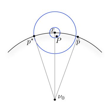
We now assume that and show this is not possible. First observe that . These expressions imply that , and thus
a contradiction. The last steps follows by setting
and solving for ,
Since , so we have .
Recall that an -kernel sample of satisfies
Theorem C.9.
If then . If is an -kernel sample of then .
C.2 Approximating the Minimum Kernel Distance Point
The goal in this section is to find a point that approximately minimizes the kernel distance to a point set . We assume here contains points and describes a measure made of Dirac mass at each with weight (this is the empirical measure defined in Section 1.1). Let . Since , for simplicity in notation, we work with point set instead of for the remaining of this section. That is, we define . Note that is chosen over all of , as the bound in Theorem C.9 is not sufficient when choosing a point from . In particular, for any , we want a point such that .
Note that Agarwal et al. [1] provide an algorithm that with high probability finds a point such that in time . However this point is not sufficient for our purpose (that is, does not satisfy the condition ), since yields
since in general it is not true that , as would be required.
First we need some structural properties. For each point , define a radius }, where is a ball of radius centered at . In other words, it is the largest radius such that at most half of points in are within . Let be the point in such that . In other words, is a point such that no more than points in satisfy . Finally it is useful to define which is where ; in particular .
We now need to lower bound in terms of . Lemma C.7 already provides a bound in terms of the closest point for any . We follow a similar construction here.
Lemma C.11.
Consider a set of vectors in a Hilbert space endowed with norm and inner product . Let each have norm . Consider weights such that and . Let . Define a partition of with and such that is the smallest set such that , and for all and we have . Let . Then
Proof C.12.
For ease of notation, we assume that for all , and let . Let . Let be a norm vector that has . Since and , let and (for . By definition, we also have . We can decompose as
The last inequality holds by . Then since we can solve for as
Lemma C.13.
Using as defined above, then .
Proof C.14.
Let map points in to the reproducing kernel Hilbert space (RKHS) defined by kernel . This space has norm defined on a set of points and inner product . Let be the representation of a set of points in . Note that . We can now apply Lemma C.11 to with weights and , and norm . Finally note that we can use since represents the set of points which are further or equal to than is . In addition, by the property of RKHS, . Hence .
Lemma C.15.
.
Proof C.16.
Now we place a net on ; specifically, it is a set of points such that for some that (we refer to this inequality as the net condition, therefore, is a set of points such that some points in it satisfy the net condition). Since is -Lipschitz, we have . This ensures that some point satisfies , and can serve as . In other words, is guaranteed to contain some point that can serve as .
Note that must be in , the convex hull of . Otherwise, moving to the closest point on decreases the distance to all points, and thus increases , which cannot happen by definition of . Let be the diameter of (the distance between the two furthest points). Clearly for some we must have .
Also note that must be within a distance to some , otherwise for , we can bound which means is not a maximum. The first inequality is by definition of , the second by assuming .
Let be the ball centered at with radius . Let . So must be in . We describe a net construction for one ball ; that is for any such that is the closest point to , then some point satisfies . Thus if this point , the correct property holds, and we can use the corresponding as . Then , and is at most times the size of . Let be the smallest integer such that . The net will be composed of , where .
Before we proceed with the construction, we need an assumption: That is a bounded quantity, it is not too small. That is, no point has more than half the points within an absolute radius . We call the median concentration.
Lemma C.17.
A net can be constructed of size so that all points satisfy for some .
If , then such a point satisfies the net condition, that is there is a point such that .
Proof C.18.
For all points , they must have , otherwise is completely inside , and cannot have enough points. Within we place the net so that all points satisfy for some . Now , and since (for , via Lemma 5.5), thus the net ensures if , then some is sufficiently close to .
Since fits in a squared box of side length , then we can describe as an axis-aligned grid with points along each axis. We define two cases to bound . When then we can set
Otherwise,
Then we need .
When we still need to handle the case for where the annulus . For a point if then . We only worry about the net on for these points where is the closest point, the others will be handled by another for and .
Recall is the smallest integer such that .
Lemma C.19.
A net can be constructed of size so that all points where , satisfy for some .
If , then such a point satisfies the net condition, that is there is a point such that .
Proof C.20.
We now consider the annuli which cover . Each has volume . For any we have , so the Euclidean distance to the nearest can be at most . Thus we can cover with a net of size based on two cases again. If then
Otherwise
Since , then the total size of , the union of all of these nets, is . In the first case dominates the cost and in the second case it is .
Thus the total size of is where . It just remains to bound . Given that no more than points are collocated on the same spot (which already holds by being a bounded quantity), then for all , . The value is known as the spread of a point set, and it is common to assume it is an absolute bounded quantity related to the precision of coordinates, where is not too large. Thus we can bound .
Theorem C.21.
Consider a point set with points, spread , and median concentration . For any , in time we can find a point such that .
Proof C.22.
Using Lemma C.17 and Lemma C.19 we can build a net of size such that some satisfies . Lemma C.15 ensures that this satisfies since is -Lipschitz.
We can find such a and set it as by evaluating for all and taking the one with largest value. This takes for each .
We claim that in many realistic settings . In such a case the algorithm runs in time. If , then over half of the measure described by will essentially behave as a single point. In many settings is drawn uniformly from a compact set , so then choosing so that more than half of has negligible diameter compared to will cause that data to be over smoothed. In fact, the definition of can be modified so that this radius never contains more than any points for any constant , and the bounds do not change asymptotically.
Appendix D Details on Reconstruction Properties of Kernel Distance
In this section we provide the full proof for some statements from Section 4.
D.1 Topological Estimates using Kernel Power Distance
For persistence diagrams of sublevel sets filtration of and the weighted Rips filtration to be well-defined, we need the technical condition (proved in Lemma D.1 and D.3) that they are -tame. Recall a filtration is -tame if for any , the homomorphism between and induced by the canonical inclusion has finite rank [12, 16].
Lemma D.1.
The sublevel sets filtration of is -tame.
Proof D.2.
The proof resembles the proof of -tameness for distance to measure sublevel sets filtration (Proposition 12, [8]). We have shown that is -Lipschitz and proper. Its properness property implies that any sublevel set (for ) is compact. Since is triangulable (i.e. homeomorphic to a locally finite simplicial complex), there exists a homeomorphism from to a locally finite simplicial complex . For any , since is compact, we consider the restriction of to a finite simplicial complex that contains . The function is continuous on , therefore its sublevel set filtration is -tame based on Theorem 2.22 of [16], which states that the sublevel sets filtration of a continuous function (defined on a realization of a finite simplicial complex) is -tame. Extending the above construction to any , the sublevel sets filtration of is therefore -tame. As homology is preserved by homeomorphisms , this implies that the sublevel sets filtration of is -tame.
Setting , Lemma D.1 implies that the sublevel sets filtration of is also -tame.
Lemma D.3.
The weighted Rips filtration is -tame for compact subset .
Proof D.4.
Since is compact subset of , is -tame based on Proposition 32 of [16], which states that the weighted Rips filtration with respect to a compact subset in metric space and its corresponding weight function is -tame.
Setting , , Lemma D.3 implies that the weighted Rips filtration is well-defined.
D.2 Inference of Compact Set with the Kernel Distance
Suppose is a uniform measure on a compact set in . We now compare the kernel distance with the distance function to the support of . We show how approximates , and thus allows one to infer geometric properties of from samples from .
For a point , the distance function measures the minimum distance between and any point in , . The point that realizes the minimum in the definition of is the orthogonal projection of on . The location of the points that have more than one projection on is the medial axis of [54], denoted as . Since resides in the unbounded component , it is referred to as the outer medial axis similar to the concept found in [28]. The reach of is the minimum distance between a point in and a point in its medial axis, denoted as . Similarly, one could define the medial axis of (i.e. the inner medial axis which resides in the interior of ) following definitions in [53], and denote its associated reach as . The concepts of reach associated with the inner and outer medial axis of capture curvature information of the compact set.
Recall that a generalized gradient and its corresponding flow to a distance function are described in [14] and later adapted for distance-like functions in [15]. Let be a distance function associated with a compact set of . It is not differentiable on the medial axis of . It is possible to define a generalized gradient function coincides with the usual gradient of where is differentiable, and is defined everywhere and can be integrated into a continuous flow . Such a flow points away from , towards local maxima of (that belong to the medial axis of ) [54]. The integral (flow) line of this flow starting at point in can be parameterized by arc length, , and we have .
Lemma D.5 (Lemma 4.5).
Given any flow line associated with the generalized gradient function , is strictly monotonically increasing along for sufficiently far away from the medial axis of , for and . Here denotes a ball of radius , , and suppose .
Proof D.6.
Since is always positive, and where is a constant that depends only on , , and , then it is sufficient to show that is strictly monotonically decreasing along .
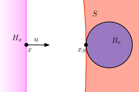
Let be the negative of the direction of the flow line at (i.e is a unit vector that points towards ). We show that is strictly monotonically increasing along . Informally, we will observe that all parts of that are “close” to are in the direction , and that these parts dominate the gradient of along . We now make this more formal by describing two quantities, and , illustrated in Figure 6.
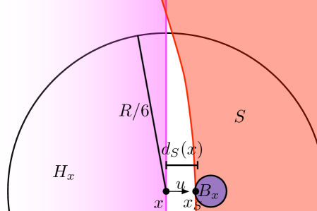
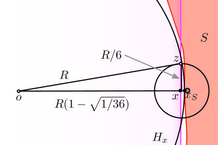
For a point , let ; since is not on the medial axis of , is uniquely defined and points in the direction of . First, we claim that there exists a ball of radius incident to that is completely contained in . This holds since . In addition, since , no part in is further than from . Second, we claim that no part of within () of (this includes ) is in the halfspace with boundary passing through and outward normal defined by . To see this, let be the center of a ball with radius that is incident to but not in , refer to such a ball as . This implies that points , and are colinear. Then a ball centered at with radius should intersect outside of , and in the worst case, on the boundary of . This holds as long as ; see Figure 6. Define .
Now we examine the contributions to the directional derivative of along the direction of from points in and , respectively. Such a directional derivative is denoted as . Recall and is a uniform measure on , . For any point , we define . Therefore .
We now examine the contribution to from points in , . First, for all points , since , we have . Second, at least half of points (that covers half the volume of ) is at least away from , and correspondingly for these points . We have . Given , we have . Denote .
We now examine the contribution to from points in , . For any point (including ), . Let so we have . Since this bound on is maximized at , under the condition , we can set to achieve the bound for (that is, for all ). Now we have , leading to . Denote .
Since only the points could possibly reside in and thus can cause to be negative, we just need to show that . This can be confirmed by plugging in , and using some algebraic manipulation.
Appendix E Lower Bound on Wasserstein Distance
We note the next result is a known lower bounds for the Earth movers distance [23][Theorem 7]. We reprove it here for completeness.
Lemma E.1 (Lemma. 5.17).
For any probability measures and defined on we have
Proof E.2.
Let describes the optimal transportation plan from to . Also let be the unit vector from to . Then we can expand
The first inequality follows since is the length of a projection and thus must be at most . The second inequality follows since that projection describes the squared length of mass along the direction between the two centers and , and the total sum of squared length of unit mass moved is exactly . Note the left-hand-side of the second inequality could be larger since some movement may cancel out (e.g. a rotation).