Geometric Weakly Admissible Meshes, Discrete Least Squares Approximations and Approximate Fekete Points††thanks: Supported by the “ex-” funds of the University of Padova, by the INdAM GNCS and NSERC, Canada.
Abstract
Using the concept of Geometric Weakly Admissible Meshes (see §2 below) together with an algorithm based on the classical QR factorization of matrices, we compute efficient points for discrete multivariate least squares approximation and Lagrange interpolation.
2000 AMS subject classification: 41A10, 41A63, 65D05, 65D15, 65Y20. Keywords: Admissible Meshes, Discrete Least Squares Approximation, Approximate Fekete Points, Multivariate Polynomial Interpolation.
1 Introduction.
In a recent paper [14], Calvi and Levenberg have developed the theory of “admissible meshes” for uniform polynomial approximation over multidimensional compact sets. Their theory is for , but here we restrict our attention to , the relevant definitions and results being easily adaptable to the general case. We begin with introducing some notation.
Suppose that is compact. We will require that not be too small, that is, that it is polynomial determining, i.e., if a polynomial is zero on then it is identically zero. This will certainly be the case if contains some open ball, as will be the case for all our examples.
We will let denote the space of polynomials of degree at most in real variables.
Then, a Weakly Admissible Mesh (WAM) of is a sequence of discrete subsets such that
| (1) |
where and the constants have (at most) polynomial growth in i.e.,
| (2) |
and
| (3) |
Throughout the paper, . When is bounded, , we speak of an Admissible Mesh (AM). It is easy to see that (W)AMs satisfy the following properties (cf. [14]):
-
•
for affine mappings of the image of a WAM is also a WAM, with the same constant
-
•
any sequence of sets containing , with polynomially growing cardinalities, is a WAM with the same constants
-
•
any sequence of unisolvent interpolation sets whose Lebesgue constant grows at most polynomially with is a WAM, being the Lebesgue constant itself
-
•
a finite union of WAMs is a WAM for the corresponding union of compacts, being the maximum of the corresponding constants
-
•
a finite cartesian product of WAMs is a WAM for the corresponding product of compacts, being the product of the corresponding constants.
As shown in [14], such meshes are very useful for polynomial approximation in the max-norm on . In fact, given the classical least-square polynomial approximant on to a function , say , we have that
| (4) |
see [14, Thm. 1]. Moreover, Fekete points (points that maximize the Vandermonde determinant) extracted from a WAM have a Lebesgue constant with the bound
| (5) |
that is times the classical bound for the Lebesgue constant of true (continuum) Fekete points; see [14, §4.4]. Recently, a new algorithm has been proposed for the computation of Approximate Fekete Points, using only standard tools of numerical linear algebra such as the QR factorization of Vandermonde matrices, cf. [7, 30].
These results show that in computational applications it is important to construct WAMs with low cardinalities and slowly increasing constants . We recall that is always possible to construct easily an AM on compact sets that admit a Markov polynomial inequality, as is shown in the key result [14, Thm. 5]. There are wide classes of such compacts, for example convex bodies, and more generally sets satisfying an interior cone condition, but the best known bounds for the cardinality of the resulting meshes grow like , where is the exponent of the Markov inequality (typically in the real case). This means that, for example, for a 3-dimensional cube or ball one should work with points, a number that becomes practically intractable already for relatively small values of (recall that the number of points determines the number of rows of the Least Squares (non-sparse) matrices). But already in dimension two, working with points makes the construction of polynomial approximants at moderate values of computationally rather expensive.
The properties of WAMs listed above (concerning finite unions and products) suggest an alternative: we can obtain good meshes, even on complicated geometries, if we are able to compute WAMs of low cardinality on standard compact “pieces”. For example, it is immediate to get a WAM with for the -dimensional cube, as the tensor-product of 1-dimensional Fekete (or Chebyshev) points.
In this paper we introduce the notion of geometric WAM, that is a WAM obtained by a geometric transformation of a suitable low-cardinality discretization mesh on some reference compact set, like the -dimensional cube. Such geometric WAMs, as well as those obtained by finite unions and products, can be used directly for discrete Least Squares approximation, as well as for the extraction of good interpolation points by means of the Approximate Fekete Points algorithm described in [7, 30], on compact sets with various geometries.
In Section 2 we illustrate the idea of geometric WAMs by several examples in , the disk, triangles, trapezoids, and polygons. In Section 3 we prove a general result on the asymptotics of approximate Fekete points extracted from WAMs by the greedy algorithm in [7, 30]. Finally, in Section 4 we present some numerical results concerning discrete Least Squares approximation and interpolation at Approximate Fekete Points on geometric WAMs.
2 Geometric WAMs.
Let and be compact subsets of ,
| (6) |
and a sequence of discrete subsets of . A geometric WAM of is a sequence
| (7) |
where the defining properties of a WAM, (1)-(3) stem from the “geometric structure” of , , , and . To make more precise this still somewhat vague notion, we give some illustrative examples in , where the reference compact is a rectangle.
2.1 The disk.
A geometric WAM of the disk can be immediately obtained by working with polar coordinates, i.e., by considering the map
| (8) |
We now state and prove the following
Proposition 1
The sequence of polar grids
gives a WAM of the unit disk, such that and .
Proof. Observe that given a polynomial , when restricted to the disk in polar coordinates, becomes a polynomial of degree in for any fixed , and a trigonometric polynomial of degree in for any fixed . Recall that Chebyshev-Lobatto points are near-optimal for 1-dimensional polynomial interpolation, and equally spaced points are near-optimal for trigonometric interpolation, both having a Lebesgue constant ; cf. [18, 28]. Now, for every we can write
where is independent of since the are the Chebyshev-Lobatto points in Further
where is independent of since the are equally spaced points in Thus
i.e., is a WAM for the disk with . We conclude by observing that the number of distinct points in is, due to the fact that .
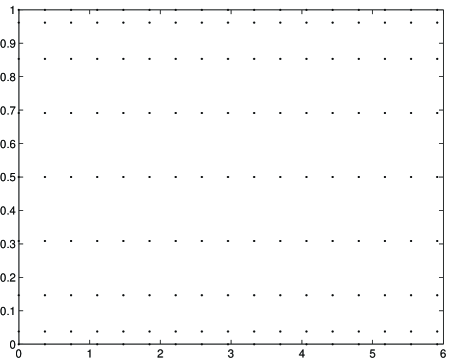
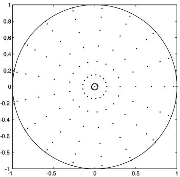
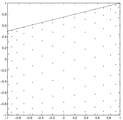
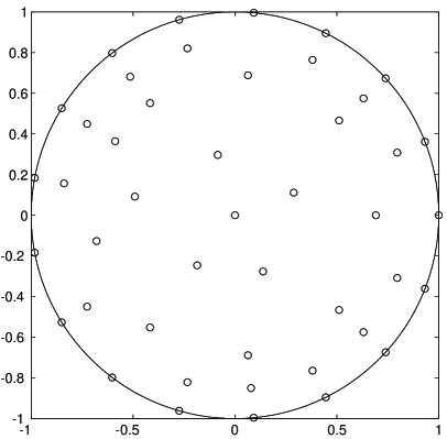
In Figure 1, we display the polar grid and the WAM in the unit disk for ( points and points, respectively). In view of the structure of and , the points of the geometric WAM cluster at the boundary and at the center of the disk. Note that this technique can also be used to construct geometric WAMs for annuli and even a ball in higher dimensions. However we will not pursue this here.
2.2 Polynomial maps.
In the case that is a polynomial map, we can give the following general
Proposition 2
Let be a WAM of , and a surjective polynomial map of degree , i.e., with . Then , with , is a WAM of such that .
Proof. Observing that for every there exists some such that , and that for every the composition is a polynomial of degree , we have
2.2.1 Triangles.
We begin by observing that for the square several WAMs formed by good interpolation points are known, namely
-
•
tensor-products of 1-dimensional near-optimal interpolation points, such as Chebyshev-Lobatto points, Gauss-Lobatto points, and others;
- •
All these WAMs have , but the Padua points have minimal cardinality , whereas the cardinality of tensor-product points is . We recall that, given the 1-dimensional Chebyshev-Lobatto points
| (9) |
the Padua points of degree are given by the union of two Chebyshev-Lobatto grids
| (10) |
There is a simple quadratic map from the square to any triangle with vertices , , , namely the Duffy transformation (cf. [16])
| (11) |
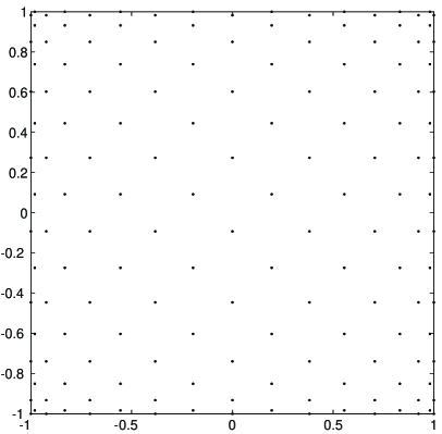
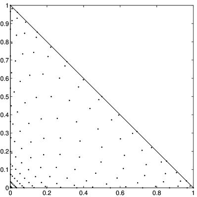
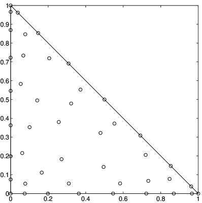
which collapses one side of the square (here ) onto a vertex of the triangle (here ). By this map, the Padua points of the square (cf. (10)) are transformed to the WAM of the triangle, with constants . The number of distinct points in is . In Figure 2, we display the WAMs in the square and in the unit simplex for ( points and points, respectively). In view of the properties of the Padua points, the points of the geometric WAM cluster at the sides and especially at the vertices of the simplex.
2.2.2 Polynomial trapezoids.
We consider here bidimensional compact sets of the form
| (12) |
where . A polynomial map of degree from the square onto is
| (13) |
Observe that a triangle could be treated (up to an affine tranformation) as a degenerate linear trapezoid.
By Proposition 2, the Padua points of the square are mapped to the WAM of the polynomial trapezoid, with and .
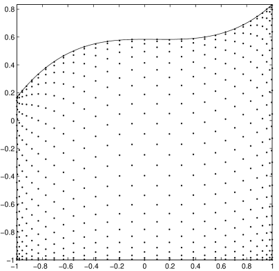
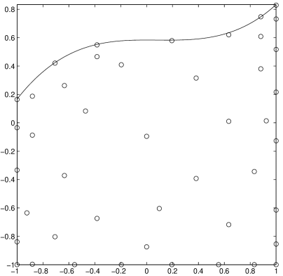
In Figure 12 we show the WAMs and obtained by mapping the Padua points onto a linear trapezoid (quadratic map) and a cubic trapezoid (quartic map), again for (the numbers of points are and , respectively). As expected, we observe clustering at the sides and at the vertices of the trapezoids. Notice that it could happen that , namely when the graphs of and intersect at some (the Chebyshev-Lobatto points of ).
2.2.3 Finite unions: polygons.
A relevant example concerning finite unions is given by polygons, which are very important in applications such as 2-dimensional computational geometry. As known, any simple (no interlaced sides) and simply connected polygon with vertices can be subdivided into triangles, and this can be done by fast algorithms, cf. e.g. [19, 26]. Once this rough triangulation is at hand, we can immediately obtain a geometric WAM for the polygon by union of the geometric WAMs constructed by mapping the Padua points on the triangles, with and , in view of the basic properties of WAMs and the results of Section 2.2.1. The points of the union WAM will cluster especially at the triangles common sides and vertices.
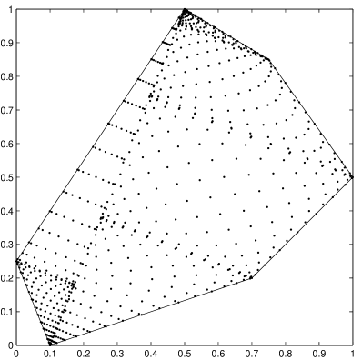
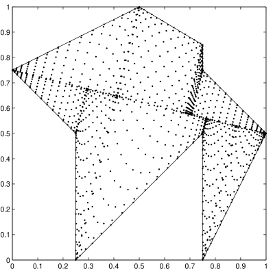
A similar approach is to subdivide into linear trapezoids, where we again obtain by finite union a geometric WAM for the polygon with and (see Section 2.2.2). In Figure 4 we show geometric WAMs generated by subdivision into linear trapezoids of a convex and a nonconvex polygon, for . The method adopted, which works for a wide class of polygons, is that used for the generation of algebraic cubature points in [29], where the trapezoidal panels are obtained simply by orthogonal projection of the sides on a fixed reference line (observe that the points cluster at the sides and at the line).
3 Approximate Fekete Points from WAMs.
In this section we go to the general setting of polynomial interpolation in several complex variables. Suppose that is a compact polynomially determining set. If is a basis for where and is a discrete subset of cardinality then
| (14) |
is called the corresponding Vandermonde determinant. If the determinant is non-zero then we may form the so-called fundamental Lagrange interpolating polynomials
| (15) |
Indeed, then for any the polynomial (of degree )
| (16) |
interpolates at the points of i.e., A set of points which maximize as a function of are called Fekete points of degree for and have the special property that (and hence Lebesgue constant bounded by ) and provide a very good (often excellent) set of interpolation points for However, they are typically very difficult to compute, even for moderate values of
For any determining subset (thought of as a sufficiently good discrete model of ) the algorithm introduced by Sommariva and Vianello in [30] and studied by Bos and Levenberg in [7] selects, in a simple and efficient manner, a subset of Approximate Fekete Points, and hence provides a practical alternative to true Fekete points, The optimization problem is nonlinear, and large-scale already for moderate values of , but the algorithm is able to give an approximate solution using only standard tools of numerical linear algebra.
We sketch here the algorithm, in a Matlab-like notation. The goal is extracting a maximum volume square submatrix from the rectangular Vandermonde matrix
| (17) |
where the polynomial basis and the array of points have been (arbitrarily) ordered. The core is given by the following iteration: Algorithm greedy (max volume submatrix of a matrix , )
-
•
-
•
-
–
“select the largest norm column ”; ;
-
–
“remove from every column of its orthogonal projection onto ;
end;
-
–
which works when is full rank and gives an approximate solution to the NP-hard maximum volume problem; cf. [15]. Then, we can extract the Approximate Fekete Points
The algorithm can be conveniently implemented by the well-known QR factorization with column pivoting, originally proposed by Businger and Golub in 1965 [10], and used for example by the Matlab “mldivide” or “” operator in the solution of underdetermined linear systems (via the LAPACK routine DGEQP3, cf. [22, 25]).
Some remarks on the polynomial basis are in order. First note that if is some other basis of then there is a transition matrix so that . It is easy to verify that then
Hence true Fekete points do not depend on the basis used and also the Lagrange polynomials of (15) are independent of the basis. Moreover, if and are two point sets for which
for some constant then the same inequality holds using the basis i.e.,
since both sides scale by the same factor.
The greedy Algorithm described above is in general affected by the basis. But this not withstanding, in the theorem below we show that if the initial set is a WAM, then the so selected approximate Fekete points, using any basis, and the true Fekete points for both have the same asymptotic distribution.
Theorem 1
Suppose that is compact, non-pluripolar, polynomially convex and regular (in the sense of Pluripotential theory) and that for is a WAM. Let be the Approximate Fekete Points selected from by the greedy Algorithm of [30], using any basis We denote by the sum of the degree of the monomials of degree at most i.e., Then
(1) the transfinite diameter of
and
(2) the discrete probability measures converge weak-* to the pluripotential-theoretic equilibrium measure of .
Remark. For , ; for the unit circle , . If is compact, then is automatically polynomially convex. We refer the reader to [21] for other examples and more on complex pluripotential theory.
By
we will mean the Vandermonde determinant computed using the standard monomial basis.
Note also that a set of true Fekete points is also a WAM and hence we may take in which case the algorithm will select (there is no other choice) and so the true Fekete points must necessarily also have these two properties.
Proof. We suppose that is a set of true Fekete points for Suppose further that is a set of true Fekete points of degree for and that are the corresponding Lagrange polynomials. Then,
It follows that the associated Lebesgue constants
and hence, since is of polynomial growth,
By Theorem 4.1 of [3]
| (18) |
By Zaharjuta’s famous result [36], we also have
| (19) |
Further, by [15], we have (cf. the remarks on bases preceeding the statement of the Theorem)
and hence
as
4 Numerical results.
In this section, we present a suite of numerical tests concerning discrete least squares approximation on geometric WAMs and polynomial interpolation at Approximate Fekete Points extracted from them. The tests concern the 2-dimensional compact sets discussed in Section 2, that are the unit disk, the unit simplex, a linear and a cubic trapezoid, a convex and a nonconvex polygon; see Figures 1-4. All the tests have been done in Matlab (see [25]), by an Intel-Centrino Duo T-2400 processor with 1 Gb RAM.
In order to compute the Approximate Fekete Points, we have actually used a refined version of the greedy algorithm of the previous section, which is sketched below. Algorithm greedy with iterative QR refinement of the basis
-
•
take the Vandermonde matrix in (17);
-
•
-
•
end
-
-
•
(the choice of is irrelevant in practice)
-
•
The greedy algorithm is implemented directly by the last row above (in Matlab), irrespectively of the actual value of the vector , and produces a set of Approximate Fekete Points . The for loop above implements a change of polynomial basis from to the nearly-orthogonal basis with respect to the discrete inner product , whose main aim is to cope possible numerical rank-deficiency and severe ill-conditioning arising with nonorthogonal bases (usually or iterations suffice); for a complete discussion of this algorithm we refer the reader to [30].
In Figures 5-7 we display the Approximate Fekete Points of degree extracted form the geometric WAMs of Figures 1-4. The computational advantage of working with a Weakly Admissible Mesh instead of an Admissible Mesh is shown in Table 1, where we show the cardinalities of the relevant discrete sets in the case of the disk. We recall that, following [14, Thm.5], it is always possible to construct an AM for a real -dimensional compact set that admits a Markov polynomial inequality with exponent , by intersection with a uniform grid of stepsize . In particular, convex compact sets have , and it is easily seen from the Markov polynomial inequality valid for every and in the disk, and the proof of [14, Thm.5], that it is sufficient to take a stepsize . The cardinality of the corresponding AM is then , to be compared with the cardinality of the geometric WAM (see Section 2.1). For example, at degree an AM for the disk has more than 2 millions points, whereas the geometric WAM has less than 2 thousands points.
| points | ||||||
|---|---|---|---|---|---|---|
| AM | 2032 | 31700 | 159692 | 503868 | 1229072 | 2547452 |
| WAM | 60 | 220 | 480 | 840 | 1300 | 1860 |
| AFP | 21 | 66 | 136 | 231 | 351 | 496 |
In Table 2, we show the Lebesgue constants of the Approximate Fekete Points extracted from the geometric WAMs for the disk at a sequence of degrees, using the algorithm above with different polynomial bases. Such Lebesgue constants have been evaluated numerically on a suitable control mesh, much finer than the extraction mesh. Without refinement iterations, the best results are obtained with the Logan-Shepp basis, which, as is well known, is orthogonal for standard Lebesgue measure (cf. [23]). On the contrary, with the monomial basis we face severe ill-conditioning and even numerical rank deficiency of the Vandermonde matrix, and we get the worst Lebesgue constants. After two refinement iterations, however, we are working in practice with a discrete orthogonal basis, the corresponding Vandermonde matrices are not ill-conditioned, and the Lebesgue constants improve and stabilize. Observe that their growth is much slower than that of the theoretical bound (5).
| basis | ||||||
|---|---|---|---|---|---|---|
| Mon(0) | 7 | 21 | 34 | 869 | ||
| Mon(2) | 5 | 24 | 32 | 42 | 60 | 81 |
| Che(0) | 9 | 23 | 30 | 91 | 1321 | |
| Che(2) | 5 | 24 | 32 | 42 | 60 | 81 |
| LoS(0) | 7 | 20 | 32 | 52 | 87 | 119 |
| LoS(2) | 5 | 24 | 32 | 42 | 60 | 81 |

In Table 3 we compare, for the three test functions below, the errors (in the uniform norm) of discrete least squares approximation on the AM and on the WAM of the disk, and of interpolation at the Approximate Fekete Points extracted from the WAM (with two refinement iterations). The test functions exhibit different regularity: the first is analytic entire, the second is analytic nonentire (a bivariate version of the classical Runge function), the third is but has a singularity of the second derivatives at the origin.
-
•
test function 1:
-
•
test function 2:
-
•
test function 3:
The Vandermonde matrices have been constructed using the product Chebyshev basis. Both the least squares and the interpolation polynomial coefficients have been computed by the standard Matlab “backslash” solver, and the errors have been evaluated on a suitable control mesh.
| points | |||||||
| test 1 | LS AM | 9E-4 | 3E-10 | ||||
| LS WAM | 5E-4 | 1E-10 | 3E-15 | 7E-15 | 6E-15 | 2E-14 | |
| interp AFP | 1E-3 | 3E-10 | 2E-15 | 2E-15 | 2E-15 | 3E-15 | |
| test 2 | LS AM | 4E-1 | 1E-1 | ||||
| LS WAM | 5E-1 | 7E-2 | 5E-2 | 6E-3 | 4E-3 | 5E-4 | |
| interp AFP | 5E-1 | 7E-2 | 5E-2 | 6E-3 | 4E-3 | 5E-4 | |
| test 3 | LS AM | 2E-2 | 2E-3 | ||||
| LS WAM | 2E-2 | 1E-3 | 7E-4 | 1E-4 | 2E-4 | 4E-5 | |
| interp AFP | 2E-2 | 1E-3 | 7E-4 | 1E-4 | 2E-4 | 4E-5 |
Notice that with the AM we have computational failure (“out of memory”) in our computing system already at degree , due to the large cardinality of the discrete set; see Table 1. The least squares error on the WAM is close to that on the AM (when comparable), which shows that geometric WAMs are a good choice for polynomial approximation, with a low computational cost. It is worth observing that in the theoretical estimate (4) we even have for the AM, and for the WAM, but we recall that these are overestimates, the term being in some way “artificial” (cf. [14, Thm.2]).


The following tables are devoted to numerical tests on the other domains. First, in Table 4 we show the Lebesgue constants of the Approximate Fekete Points extracted from the geometric WAMs described in Section 2. Again, the growth is much slower than that of the theoretical bound (5).
As for the simplex, the Lebesgue constant of our Approximate Fekete Points points is larger than that of the best points known in the literature. The case of the simplex has been widely studied and several specialized approaches have been proposed for the computation of Fekete or other good interpolation points, due to the relevance in the numerical treatment of PDEs by spectral-element and high order finite-element methods: see e.g. [20, 27, 33, 35] and references therein.
On the other hand, our method for computing Approximate Fekete Points via geometric WAMs is quite general and flexible, since it allows to work on a wide class of compact sets and, differently from other computational approaches, up to reasonably high interpolation degrees. The good quality of the discrete sets used for least squares approximation and for interpolation is evidenced by Tables 5-9. We observe that the singularity of the third test function is in the interior of the domains, apart from the simplex where it is located at a vertex (where the discrete points cluster). This explains the better results with the simplex for this function. In the case of the two polygons, a change of variables is made in order to put the problem in the reference square .
The availability of good interpolation points in compact sets with various geometries has a number of potential applications. One for example is connected to numerical cubature. Indeed, when the moments of the underlying polynomial basis are known [29, 31], cubature weights associated to the Approximate Fekete Points can be computed as a by-product of the algorithm, simply by using the moments vector as right-hand side . This gives an algebraic cubature formula, that can be used directly, or as a starting point towards the computation of a minimal formula, by the method developed in [34].
Another relevant application concerns the numerical treatment of PDEs, where a renewed interest is arising in global polynomial methods, such as collocation and discrete least squares methods, over general domains (see, e.g., [24]). Recently, Approximate Fekete Points have been successfully used for discrete least squares discretization of elliptic equations [37]. Moreover, again in the context of numerical PDEs, Approximate Fekete Points for polygons could play a role in connection with discretization methods on polygonal (non simplicial) meshes (see, e.g., [32] and references therein).
| set | ||||||
|---|---|---|---|---|---|---|
| disk | 5 | 24 | 32 | 42 | 60 | 81 |
| simplex | 5 | 15 | 25 | 48 | 62 | 80 |
| linear trap | 6 | 19 | 34 | 37 | 31 | 54 |
| cubic trap | 6 | 16 | 35 | 45 | 40 | 75 |
| conv polyg | 7 | 13 | 22 | 53 | 53 | 66 |
| nonconv polyg | 5 | 18 | 36 | 35 | 45 | 80 |
| points | |||||||
|---|---|---|---|---|---|---|---|
| test 1 | LS WAM | 7E-7 | 8E-15 | 3E-15 | 4E-15 | 4E-15 | 6E-15 |
| interp AFP | 2E-6 | 2E-14 | 1E-15 | 3E-15 | 3E-15 | 5E-15 | |
| test 2 | LS WAM | 2E-2 | 5E-4 | 1E-5 | 4E-7 | 1E-8 | 4E-10 |
| interp AFP | 5E-2 | 2E-3 | 4E-5 | 2E-6 | 3E-8 | 2E-9 | |
| test 3 | LS WAM | 7E-4 | 5E-6 | 4E-7 | 8E-8 | 2E-8 | 7E-9 |
| interp AFP | 8E-4 | 2E-5 | 1E-6 | 2E-7 | 6E-8 | 3E-8 |
| points | |||||||
|---|---|---|---|---|---|---|---|
| test 1 | LS WAM | 3E-3 | 5E-9 | 1E-13 | 3E-15 | 4E-15 | 9E-15 |
| interp AFP | 8E-3 | 2E-8 | 3E-13 | 4E-15 | 3E-15 | 4E-15 | |
| test 2 | LS WAM | 2E-1 | 2E-1 | 1E-1 | 3E-2 | 1E-2 | 5E-3 |
| interp AFP | 3E-1 | 2E-1 | 2E-1 | 3E-2 | 2E-1 | 1E-2 | |
| test 3 | LS WAM | 3E-2 | 4E-3 | 2E-3 | 5E-4 | 2E-4 | 1E-4 |
| interp AFP | 5E-2 | 4E-3 | 3E-3 | 5E-4 | 3E-4 | 2E-4 |
| points | |||||||
|---|---|---|---|---|---|---|---|
| test 1 | LS WAM | 2E-3 | 6E-9 | 6E-14 | 3E-15 | 4E-15 | 5E-15 |
| interp AFP | 6E-3 | 1E-8 | 1E-13 | 5E-15 | 3E-15 | 4E-15 | |
| test 2 | LS WAM | 4E-1 | 2E-1 | 6E-2 | 3E-2 | 9E-3 | 5E-3 |
| interp AFP | 5E-1 | 2E-1 | 7E-2 | 5E-2 | 1E-2 | 6E-3 | |
| test 3 | LS WAM | 3E-2 | 3E-3 | 9E-4 | 5E-4 | 2E-4 | 2E-4 |
| interp AFP | 6E-2 | 5E-3 | 9E-4 | 7E-4 | 2E-4 | 2E-4 |
| points | |||||||
|---|---|---|---|---|---|---|---|
| test 1 | LS WAM | 7E-4 | 1E-9 | 7E-15 | 9E-15 | 1E-14 | 2E-14 |
| interp AFP | 1E-3 | 4E-9 | 6E-15 | 4E-15 | 4E-15 | 5E-15 | |
| test 2 | LS WAM | 4E-1 | 1E-1 | 4E-2 | 2E-2 | 4E-3 | 1E-3 |
| interp AFP | 5E-1 | 1E-1 | 4E-2 | 2E-2 | 9E-3 | 3E-3 | |
| test 3 | LS WAM | 2E-2 | 2E-3 | 6E-4 | 3E-4 | 1E-4 | 9E-5 |
| interp AFP | 2E-2 | 2E-3 | 6E-4 | 3E-4 | 1E-4 | 8E-5 |
| points | |||||||
|---|---|---|---|---|---|---|---|
| test 1 | LS WAM | 5E-4 | 3E-10 | 1E-14 | 2E-14 | 3E-14 | 4E-13 |
| interp AFP | 6E-4 | 5E-10 | 3E-15 | 3E-15 | 3E-15 | 4E-15 | |
| test 2 | LS WAM | 4E-1 | 2E-1 | 5E-2 | 2E-2 | 5E-3 | 1E-3 |
| interp AFP | 6E-1 | 2E-1 | 5E-2 | 2E-2 | 5E-3 | 2E-3 | |
| test 3 | LS WAM | 2E-2 | 3E-3 | 7E-4 | 3E-4 | 1E-4 | 9E-5 |
| interp AFP | 4E-2 | 3E-3 | 8E-4 | 3E-4 | 1E-4 | 7E-5 |
References
- [1] R. Berman and S. Boucksom, Equidistribution of Fekete Points on Complex Manifolds, preprint (online at: http://arxiv.org/abs/0807.0035).
- [2] A. Björk, Numerical methods for least squares problems, SIAM, 1996.
- [3] T. Bloom, L. Bos, C. Christensen and N. Levenberg, Polynomial interpolation of holomorphic functions in ℂ and , Rocky Mtn. J. Math 22 (1992), 441–470.
- [4] T. Bloom, L. Bos, N. Levenberg and S. Waldron, On the Convergence of Optimal Measures, submitted.
- [5] L. Bos, M. Caliari, S. De Marchi, M. Vianello and Y. Xu, Bivariate Lagrange interpolation at the Padua points: the generating curve approach, J. Approx. Theory 143 (2006), 15–25.
- [6] L. Bos, S. De Marchi, M. Vianello and Y. Xu, Bivariate Lagrange interpolation at the Padua points: the ideal theory approach, Numer. Math. 108 (2007), 43–57.
- [7] L. Bos and N. Levenberg, On the Approximate Calculation of Fekete Points: the Univariate Case, Electron. Trans. Numer. Anal. 30 (2008), 377–397.
- [8] L. Bos, N. Levenberg and S. Waldron, On the Spacing of Fekete Points for a Sphere, Ball or Simplex, Indag. Math., to appear// (online at: http://www.math.auckland.ac.nz/waldron/Preprints).
- [9] L. Bos, M.A. Taylor and B.A. Wingate, Tensor product Gauss-Lobatto points are Fekete points for the cube, Math. Comp. 70 (2001), 1543–1547.
- [10] P.A. Businger and G.H. Golub, Linear least-squares solutions by Householder transformations, Numer. Math. 7 (1965), 269–276.
- [11] M. Caliari, S. De Marchi and M. Vianello, Bivariate polynomial interpolation at new nodal sets, Appl. Math. Comput. 165 (2005), 261–274.
- [12] M. Caliari, S. De Marchi and M. Vianello, Bivariate Lagrange interpolation at the Padua points: computational aspects, J. Comput. Appl. Math. 221 (2008), 284–292.
- [13] M. Caliari, S. De Marchi and M. Vianello, Algorithm 886: Padua2D: Lagrange Interpolation at Padua Points on Bivariate Domains, ACM Trans. Math. Software 35-3 (2008).
- [14] J.P. Calvi and N. Levenberg, Uniform approximation by discrete least squares polynomials, J. Approx. Theory 152 (2008), 82–100.
- [15] A. Civril and M. Magdon-Ismail, Finding Maximum Volume Sub-matrices of a Matrix, Technical Report 07-08, Dept. of Comp. Sci., RPI, 2007 (online at: http://serv2.ist.psu.edu:8080/viewdoc/summary?doi=10.1.1.64.4502).
- [16] M.G. Duffy, Quadrature over a pyramid or cube of integrands with a singularity at a vertex, SIAM J. Numer. Anal. 19 (1982), 1260–1262.
- [17] C.F. Dunkl and Y. Xu, Orthogonal Polynomials of Several Variables, Encyclopedia of Mathematics and its Applications 81, Cambridge University Press, Cambridge, 2001.
- [18] V.K. Dzjadyk, S.Ju. Dzjadyk and A.S. Prypik, On the asymptotic behavior of the Lebesgue constant in trigonometric interpolation, Ukrainian Math. J. 33 (1981), 553-559.
- [19] M. Held, FIST: Fast Industrial-Strength Triangulation of Polygons, Algorithmica 30 (2001), 563–596.
- [20] J.S. Hesthaven and T. Warburton, Nodal discontinuous Galerkin methods. Algorithms, analysis, and applications, Texts in Applied Mathematics, 54, Springer, New York, 2008.
- [21] M. Klimek, Pluripotential Theory, Oxford U. Press, 1991.
- [22] LAPACK Users’ guide, SIAM, Philadelphia, 1999 (available online at http://www.netlib.org/lapack).
- [23] B.F. Logan and L.A. Shepp, Optimal reconstruction of a function from its projections, Duke Math. J. 42 (1975), 645–659.
- [24] Y. Maday, N.C. Nguyen, A.T. Patera and G.S.H. Pau, A general multipurpose interpolation procedure: the magic points, Commun. Pure Appl. Anal. 8 (2009), 383–404.
- [25] The Mathworks, MATLAB documentation set, 2008 version (available online at: http://www.mathworks.com).
- [26] A. Narkhede and D. Manocha, Graphics Gems 5, Editor: Alan Paeth, Academic Press, 1995.
- [27] R. Pasquetti and F. Rapetti, Spectral element methods on unstructured meshes: comparisons and recent advances, J. Sci. Comput. 27 (2006), 377–387.
- [28] T.J. Rivlin, An Introduction to the Approximation of Functions, Dover, 1969.
- [29] A. Sommariva and M. Vianello, Product Gauss cubature over polygons based on Green’s integration formula, BIT Numerical Mathematics 47 (2007), 441–453.
- [30] A. Sommariva and M. Vianello, Computing approximate Fekete points by QR factorizations of Vandermonde matrices, Comput. Math. Appl., to appear (online at: www.math.unipd.it/marcov/publications.html).
- [31] A. Sommariva and M. Vianello, Gauss-Green cubature and moment computation over arbitrary geometries, J. Comput. Appl. Math., to appear (online at: www.math.unipd.it/marcov/publications.html).
- [32] N. Sukumar and E.A. Malsch, Recent advances in the construction of polygonal finite element interpolants, Arch. Comput. Methods Engrg. 13 (2006), 129–163.
- [33] M.A. Taylor, B.A. Wingate and R.E. Vincent, An algorithm for computing Fekete points in the triangle, SIAM J. Numer. Anal. 38 (2000), 1707–1720.
- [34] M.A. Taylor, B.A. Wingate and L.P. Bos, A cardinal function algorithm for computing multivariate quadrature points, SIAM J. Numer. Anal. 45 (2007), 193–205.
- [35] T. Warburton, An explicit construction of interpolation nodes on the simplex, J. Engrg. Math. 56 (2006), 247–262.
- [36] V.P. Zaharjuta, Tranfinite diameter, Chebyshev constants and capacity for compacts in , Math. USSR Sbornik 25 (1975), 350 – 364.
- [37] P. Zitnan, Discrete Weighted Least-Squares Method for the Poisson and Biharmonic Problems on Domains with Smooth Boundary, Numer. Methods Partial Differential Equations, under revision (online at: http://www.math.unipd.it/marcov/CAAfek.html).