Giant thermoelectric figure of merit in multivalley high-complexity-factor LaSO
Abstract
We report a giant thermoelectric figure of merit (up to 6 at 1100 K) in -doped lanthanum oxysulphate LaSO. Thermoelectric coefficients are computed from ab initio bands within Bloch-Boltzmann theory in an energy-, chemical potential- and temperature-dependent relaxation time approximation. The lattice thermal conductivity is estimated from a model employing the ab initio phonon and Grüneisen-parameter spectrum. The main source of the large is the significant power factor which correlates with a large band complexity factor. We also suggest a possible -type dopant for the material based on ab initio calculations.
I Introduction
Thermoelectric materials, which convert heat into electricity via the Seebeck effect, have attracted considerable interest as components of power generation devices. In addition to being scalable and reliable, thermoelectric generators are silent and require no moving parts. Sufficiently cheap and efficient thermoelectric devices therefore have massive potential for waste-heat recovery in a variety of industrial and consumer processes, such as automotive exhausts, home heating, and large-scale commercial processes genref . Industrial thermoelectric devices are still comparatively expensive and inefficient, and are often relegated to niche applications despite their potential. Nonetheless, this might change in a number of ways; for example, a breakthrough material might be be found with a high conversion efficiency as measured by the figure of merit
| (1) |
where is the electrical conductivity, the Seebeck coefficient, the temperature, and , the electronic and lattice thermal conductivities. It is thus only natural that much research is aimed at finding materials with large .
In this framework, the band complexity factor has emerged as a very relevant parameter from a large-scale data-mining study gibbs . Indeed, the power factor PF = appearing in the numerator of Eq. 1 exhibits a power law increase PF as a function of . The latter is actually obtained as , where is the multiplicity, i.e., the number of equivalent extrema within the Brillouin zone, and is a measure of the anisotropy of the relevant band extremum (the ratio of geometric and harmonic averages of the diagonal elements of the mass tensor to the power of 3/2). Thus, multiple band-structure extrema (each potentially involving multiple bands) and anisotropic masses are expected to be conducive to large power factors. A quick evaluation readily shows that the most direct power-factor amplifier is the band-valley multiplicity , whereas the factor deviates significantly from 1 (isotropic case) only for energy surfaces with unusually strong anisotropy.
In this paper, we study a material with a large complexity factor (mostly due to a large ), from which follow very large PF and predicted , despite a not especially favorable lattice thermal conductivity. Lanthanum sulfoxide, LaSO, was identified as a candidate by screening a large (so far unpublished) database of calculated band extrema. Methodologically, such database searches for significant complexity factors (and especially valley multiplicity) appear to provide useful guidance in the quest for thermoelectric materials.
II Methods and results
II.1 General
The ingredients of are the electronic transport coefficients (electrical and electronic-thermal conductivity, Seebeck thermopower) obtained from the electronic structure, and the lattice thermal conductivity, which we discuss specifically in Sec. II.3.
The electronic transport coefficients are computed from the ab initio density-functional band structure as a function of temperature and doping in the relaxation-time approximation to the linearized Boltzmann transport equation, an approach known as Bloch-Boltzmann theory allen ; bt2 . We use a model of temperature- and energy-dependent relaxation time described at length in previous papers noi ; sno , as implemented in a publicly-available custom code sno ; thermocasu . We concentrate on -type doping, although -doping also gives interesting values.
II.2 Electronic structure calculations
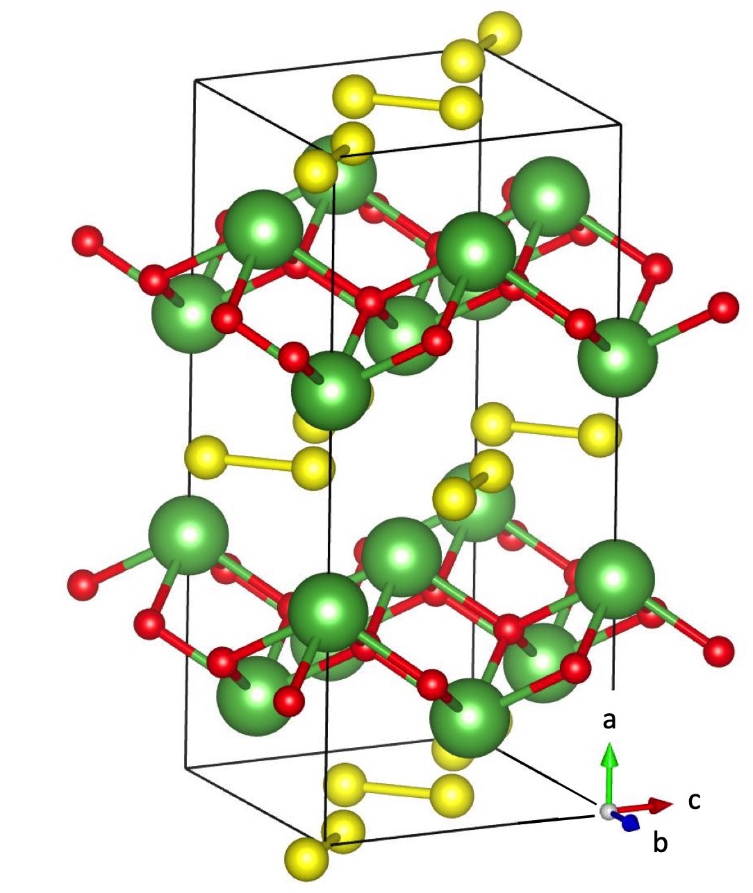
Ab initio density-functional structure optimization and band-structure calculations are performed within the generalized-gradient approximation (GGA) using the PBE functional pbe (hereafter simply labelled as GGA) and the projector augmented wave method paw using the VASP code vasp , with the La, S, and O_s datasets at the maximum suggested cutoff. LaSO has an orthorhombic structure (Fig. 1) with space group . It is optimized following quantum forces and stress in a conventional cell containing 8 formula units.
The material is made of strongly buckled La-O bonded planes intercalated in the direction by molecular-crystal-like layers of S dimers. The resulting computed lattice constants are =13.323, =5.950, and =5.945 Å. As expected, transport is found to be less efficient in the direction than in the plane.
The electronic states are calculated on a (122424) k-points grid. The minimum gap in GGA is 1.3 eV, so the -type thermoelectric coefficients are essentially unaffected by valence states (we checked this using a scissor operator which adjusts the gap to the value obtained by hybrid functional calculations, see Sec. II.7). The band structure will be discussed further in Sec. II.5.
II.3 Lattice thermal conductivity
We estimate the lattice thermal conductivity using the model of Ref. antimonides . In the present Subsection, the equation numbers refer to that paper. We compute the phonon spectrum and Grüneisen parameters from first principles using density-functional perturbation theory with the Quantum Espresso QE code, using ultrasoft pseudopotentials and GGA. The phonon-phonon relaxation time is computed from Eqs.3 and 7, where for the parameter we use the Grüneisen density of states obtained from the calculated spectrum, instead of the average Grüneisen value (which we can calculate and find to be 0.78). Beside phonon-phonon scattering, Casimir and disorder scattering can be easily introduced via Eqs. 21 and 22 (assuming for example that disorder originates from O vacancies). The sound velocity is approximated à la Debye (constant below the Debye energy , zero above); its value is the harmonic average =3134 m/s of the computed small-wavevector acoustic-branch velocities. The thermal conductivity is finally obtained from Eq.2, with energy dependence only.
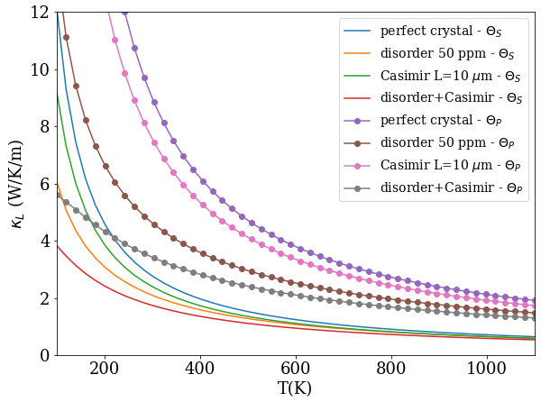
Fig. 2 shows the lattice thermal conductivity for two Debye temperatures, =215 K as obtained from our data according to the definition of Eq. 10, and =335 K with the definition by Pässler passler . The choice of changes considerably the conductivity, because the phonon-phonon scattering time depends exponentially on . In the following we will compare results obtained with for the perfect crystal with these two Debye tempeatures (the higher curves for each of the two ’s). Fig. 2 also shows for a few combinations of size and disorder parameters; weak disorder or micron-sized-crystalline Casimir scattering clearly have comparatively minor effects on the scale set by the choice of , so we will not expound upon them further.
II.3.1 Discussion
The accuracy of the estimate of to be discussed below clearly depends on the lattice conductivity, as a hypothetically much larger would directly reduce . A full ab initio computation noi is costly and impractical for this material, hence out of our present scope. Nevertheless, we reckon that the model calculation of should be sufficient for the present purposes: it has the correct asymptotic behavior; it includes the density of states and specific heat obtained ab initio, as well as the ab initio Grüneisen parameters in the relaxation time; the only model part is the relaxation time, whereby in particular the key parameter is, as mentioned, for which we use two different possible definitions; finally, the model appears to err on the side of giving too large a antimonides compared to experiments and other techniques.
Adding to this the fact that we use the worst possible (that for the crystal) to calculate below, whereas in a real material will be smaller (e.g., defected, doped, polycrystalline, etc.), we ultimately expect no significant reductions compared to our estimates (rather, even an increase). This is because the defining feature of this material is in fact the large electronic power factor.
II.4 Transport coefficients and electronic relaxation time
We compute the transport coefficients with a code thermocasu ; sno employing parts of the BoltzTrap2 bt2 transport code as libraries, and including energy- and temperature-dependent relaxation time. The ab initio bands (assumed rigid, i.e., not changing with doping or temperature) are interpolated by a Fourier-Wannier technique bt2 over a k-point grid with 64 times more points than the ab initio one, i.e. approximately equivalent to a (489696) grid.
As discussed for instance in Ref. noi , a constant relaxation time = neglects relevant physics in the electron scattering (thermal distributions, local masses, energies of phonons, and more). So we adopt a temperature- and energy-dependent relaxation time which enters the kernel of the integral in Eq. 9 of Ref. bt2 (additional details can be found in Ref. sno ). The ’s are the scattering rates of charged impurities, acoustic phonons, and polar optical phonons given in Refs. noi ; ridley1 ; ridley2 . Piezoelectric scattering is zero by symmetry ridley2 ; bilbao . We point out that there is no effective mass approximation in the transport coefficient calculations, except those implicit in the relaxation time.
The parameters entering the model for can be computed directly. The conduction-band deformation potential is =2.1 eV, the density is 5270 kgm-3 and the effective conduction mass is set to a conservatively large =0.5 . The phonon energies, dielectric tensor, and sound velocity are obtained from linear-response calculations QE as in Sec. II.3. The sound velocity is 3134 m/s as discussed in the previous Section. For the dielectric constants we use the harmonic averages of the (very similar) and components, =6.23 and =18.73 (as it turns out, the direction is quite irrelevant for thermoelectricity).
A key point is the scattering by polar (i.e. optical) phonons, which dominates the total scattering rate. The LO phonon energies are calculated directly using the linear-response approach (Sec. II.3) with non-analiticity along the crystallographic directions. Since LO phonons scatter electrons with momentum parallel to the LO polarization vector, a direction-dependent polar-phonon would be needed. To simplify the procedure, we use a set of effective LO energies (20, 27, and 30 meV) obtained as averages of the three LO groups of frequencies over the , , and directions. We deem this simplification to be quite acceptable in view of the other significant uncertainties in the calculations, such as the choice of in the lattice thermal conductivity, or our choice of using a single phonon replica in the polar-phonon scattering rate.
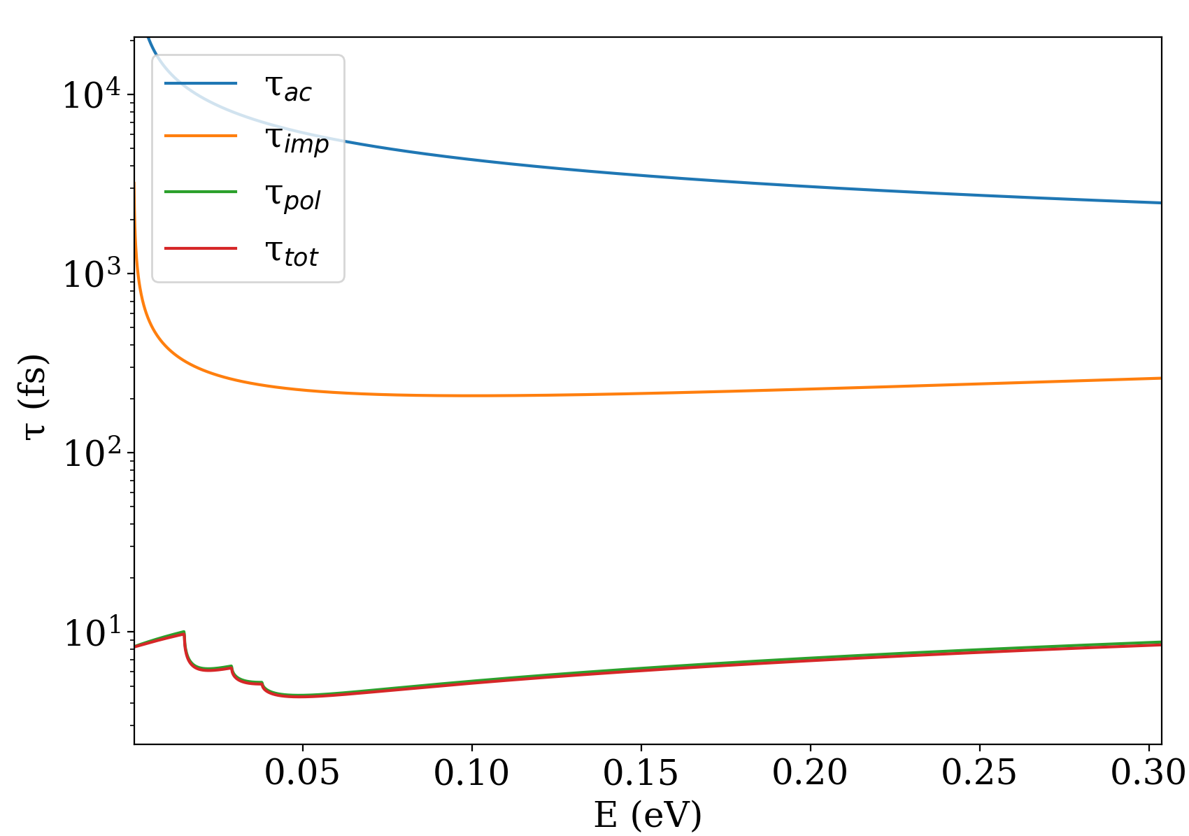
The relaxation time (,) is sketched vs. in Fig. 3. As typical of polar insulators, the polar-phonon scattering dominates, and its downward jump across the LO phonon energies is in the low energy region relevant for transport. Here, we use this relaxation time accounting self-consistently for chemical potential changes, and do not employ any average-time or constant-time approximations.
II.5 Band structure and complexity factors
We now discuss the band structure of LaSO, and two versions of the complexity factor. The first, , is a geometrical value derived from the number of valleys and the masses from the band structure. The second, , is a transport value obtained a posteriori from the calculated transport properties, with the procedure of Ref. gibbs . The data are summarized in Fig. 4, reporting the conduction-band Fermi surface of -doped LaSO at several chemical potentials, and Fig. 5, displaying the bands, the carrier density (the conduction density of states multiplied by the Fermi distribution), and the complexity factor .

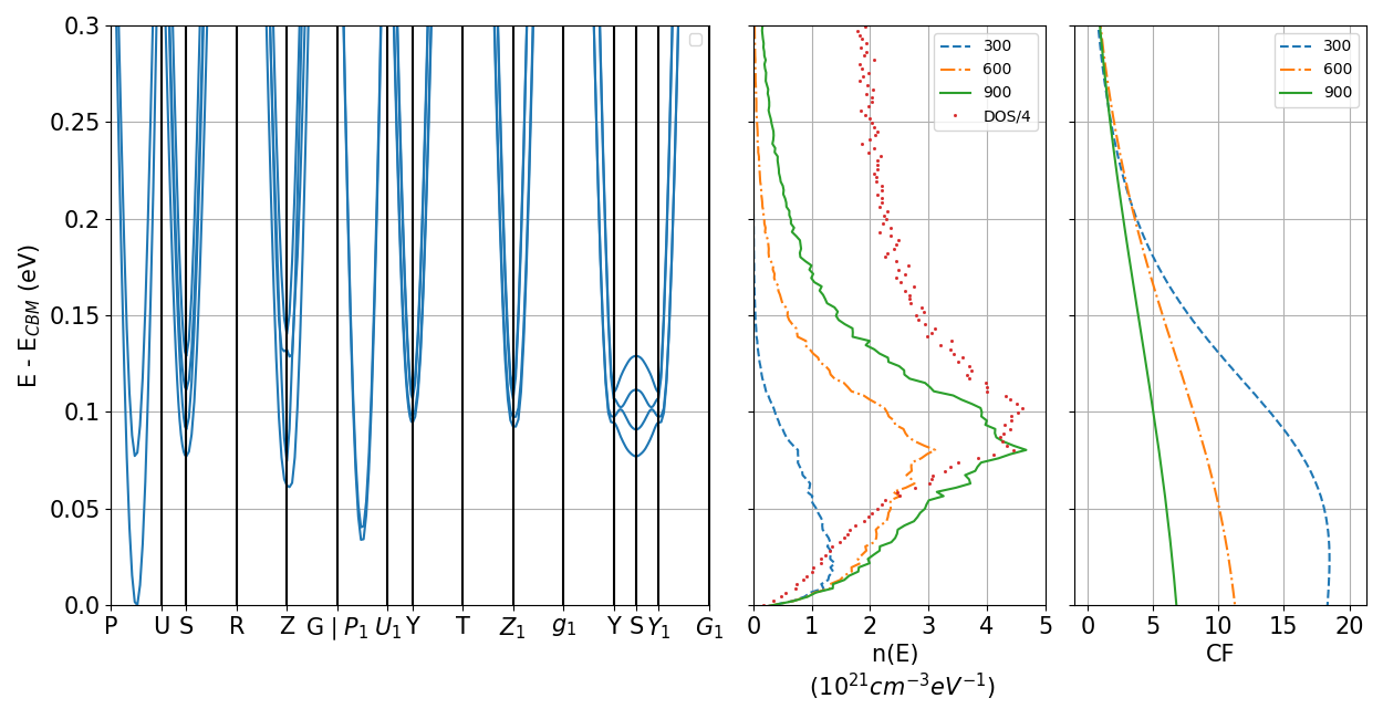
The low-energy valleys of the LaSO conduction band occur at four internal points of the Brillouin zone (BZ) and at four zone-border points (which count as two internal points). By inspection, the first four conduction states (marked in different colors in Fig. 4) provide 16 available valleys within about 150 meV of the band edge. These are visible in the Fermi surface in Fig. 4. Four valleys provided by the first band are internal to the BZ. Eight valleys, from the second band, are located on the square faces and therefore shared with adjacent BZs (hence their wight is 1/2). Eight valleys come from the third band (specifically on the segments Z-Z1 and S-Y/S-Y1, Fig. 5), and eight more from the fourth band on the same segment.
The same result is found by counting the relevant bands in Fig. 5. The stationary point on the P–U segment and its three symmetry partners contribute a total of 8 bands; points S and Z with their two symmetry partners contribute 2 bands each (accounting for their being at zone border); that amounts again to 16 available band minima.
The carrier density vs. energy (in the central panel of Fig. 5) shows that all these bands are occupied at the chemical potentials and temperatures of interest (i.e., near the lowest conduction edge, and temperatures of the order of 1 to 3 times room temperature). Accordingly, all the bands just mentioned may be considered active (i.e., contributing to the trasport), so that the effective total multiplicity of the occupied valleys is =16. From Fig. 5, we can also infer that the optimal doping level, namely the doping at which is maximal for a given , will probably fall in the low 1020 cm-3, and that the Seebeck coefficient may be interesting due to the fast rise of the density of states near the band edge.
As it turns out, the relevant directions for conduction are in the basal - plane of the material. The masses in the in-plane directions are quite isotropic, so 1, and the geometrical complexity factor is 16. If the component of the mass tensor were to be considered, a larger anisotropy would arise, resulting in 1.2-1.3, i.e., a of about 20. (The anisotropy can be appreciated, for example, from the different curvature of the bands at point S, respectively along the Y-S-Y1 segment and along the U-S-R segment.)
The transport complexity factor is in the rightmost panel of Fig. 5. It is computed from the calculated transport coefficients in the basal plane as outlined in Ref. gibbs using a constant relaxation time =10 fs, purely for consistency with Ref. gibbs . We set the scattering parameter =1 in the Seebeck coefficient model of Ref. gibbs , to take into account the dominant polar scattering we have in the present case. Similarly to most quantities in thermoelectricity, is a temperature- and chemical potential-dependent tensor. To compare it with the geometric (a scalar) we pick a low T=300 K and =0, and average over in-plane directions. at 300 K is relatively flat at low energy, and its energy average is roughly 15, in quite decent agreement with =16 obtained above. This is in line with our having considered just the in-plane, largely isotropic transport. We discuss in Sec. II.6 (especially with reference to Figs. 6 and 7) the connection of our values with the rule of thumb of Ref. gibbs .
II.6 Thermoelectric coefficients and figure of merit
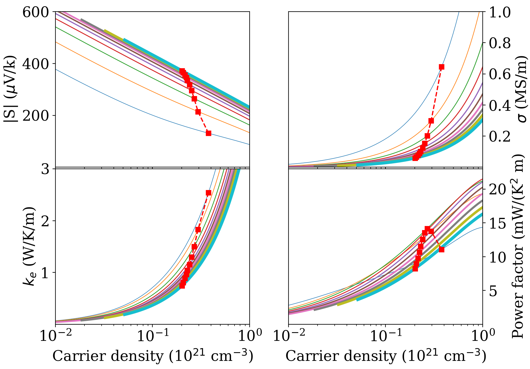
Fig. 6 reports the Seebeck coefficient, the electrical conductivity, the electronic thermal conductivity, and the power factor vs. doping and parametrized by . Fig. 7 displays the same quantities vs. at optimal doping (i.e. the doping at which is a maximum at the given temperature). For simplicity, only the component is plotted in Fig. 6. As seen in Fig. 7, the and components are very close, and the component ends up producing small power factor and , so it can be ignored.
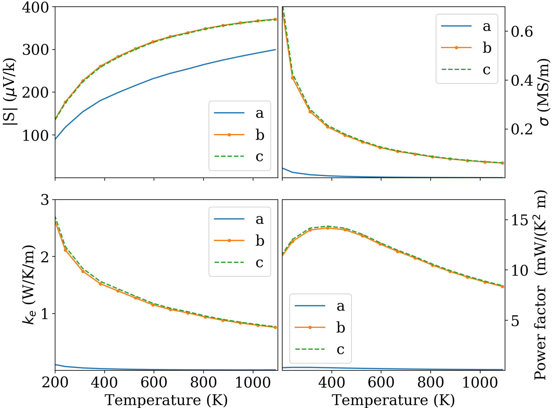
The large conductivity and Seebeck coefficient result in a large power factor for the in-plane transport, with a maximum of 15 mW/(K2m) at 400 K. We can now make contact between the large complexity factors 16 discussed in the previous Section and the rule of thumb of Gibbs et al. gibbs . For this complexity factor, Fig. 3 of Ref. gibbs suggests that the expected maximum power factor should be between 6 and 22 mW/(K2m). Using the setting of Ref. gibbs (==10 fs and =600 K), we indeed obtain a power factor of 21 mW/(K2 m); with the full relaxation time treatment, the power factor at 600 K (Fig. 7) is about 12 mW/(K2m). In both cases, our results are consistent with the general prediction gibbs .
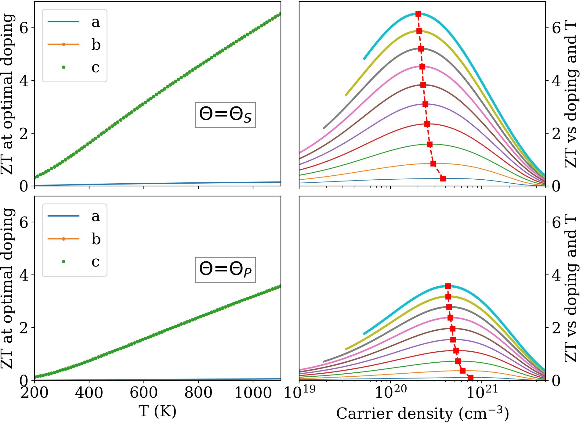
Finally, in Fig. 8, we show the tensor for the two instances of lattice thermal conductivity discussed in Sec. II.3. The left panels report the diagonal components of as a function of at optimal doping, and the right panels the component as a function of doping for different temperatures. The and components differ by only a fraction of a percent. The main results in this Figure are i) is very large, reaching values well over 3 and, respectively, 6 at high for the two versions of the lattice thermal conductivity; ii) the optimal doping is in the low to mid cm-3, depending on and . may still be rather interesting even at lower doping: for example, it is already above 2 at 800 K and 21019 cm-3 (Fig. 8, upper panel). We recall again that all coefficients refer to electrons in perfect-crystal bands, subject to scattering from phonons and charged impurities, so that no scattering is accounted for from disorder, dislocations, neutral impurities, extended defects, etc. which could affect transport in ways we cannot quantify.
II.7 Doping
Given the relatively high carrier density required to obtain interesting s, we now look into the possibility of -type doping of LaSO. Screening a number of options, we find that Hf seems to be a reasonable candidate donor.
Dopability is difficult to assess in any material, and LaSO is no exception. In particular, here we do not address possible compensation by native defects or other contaminants, but only the solubility and ionization of donors. Also, our discussion is based on equilibrium thermodynamics, so the possibility remains that epitaxial growth (which often occurs out of equilibrium), ion implantation, and certain kinds of diffusion doping processes may do better than we predict here.
Solubility and carrier concentrations are estimated from the formation energies and thermal ionization levels obtained via ab initio calculation. We use VASP, on 144-atom supercells with a 444 k-point grid and the GGA, the details being the same as in the calculations in the previous Sections. For charged states we use the simple monopole correction by Leslie and Gillan LG , with the dielectric constant calculated in Sec. II.4.
We concentrate on potential donors substituting on the La site (namely Zr, Hf, Ce, Sb, Bi, Sn, and Si) as we find that potential substitutions for O or S, such as F or Cl, tend to go interstitial or have large formation energy. Si can be discarded offhand because of its huge formation energy. Sb, Bi, and Sn can be neglected as well since they have no state (in particular no donor state) in the vicinity of the gap. This effective trivalent behavior is presumably due to the hybridization cost of the orbital, and the pyramidal bonding geometry of the La site which does not favor hybrids.
| Dopant | Hf | Zr | Zr HSE | Ce |
|---|---|---|---|---|
| +0.05 | +0.05 | +0.07 | –0.56 |
For the remaining dopants Zr, Hf, and Ce, we find the thermal levels reported in Table 1. Neutral Ce has an electron in an orbital when substituting for trivalent La, and its donor level is deep in GGA. This will not improve when using non-local-density methods (such as hybrid functionals) which remove self-interaction and tend to lower the energy of very localized occupied states. Luckily, instead, Zr and Hf have shallow thermal levels, in fact lying just above the conduction edge in GGA (although there as usual are large uncertainties in these estimates, at the very least 0.1-0.2 eV). A python notebook with the formation energies and their post processing is at https://gitlab.com/vfiore/laso-eform.
To check for the effects of more advanced exchange-correlation functionals, we calculated the thermal level for Zr using the hybrid HSE functional hse , and found a value similar to GGA. This is further confirmed by the electronic band structure, which exhibits impurity-related resonant states within the lower portion of the conduction band, at the same position both in GGA and HSE. In passing, the gaps are 1.3 eV in GGA and 2.9 eV and HSE, the difference being within 15% of that predicted by the dielectric correction rule FB .
Another interesting result of these calculations is that the upper valence band and the bottom conduction band are predominantly sulphur-like, so that conduction effectively occurs in-plane in the S layers. Carriers living in the S layer may thus be partially decoupled from charged impurities in the La-O layers, leading to a reduced impurity scattering.
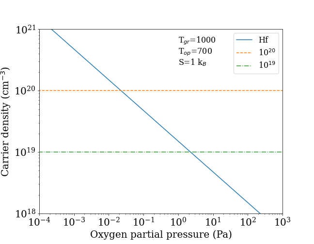
To present synthetically the results as a function of an operational quantity, we report in Fig. 9 the density of carriers vs. the oxygen partial pressure at a typical device operating temperature =700 K, and with Hf incorporated in LaSO in thermal equilibrium during growth at temperature . The rationale for this is that, as we now discuss in more detail, the partial pressure is related to the formation energy of the donor via the oxygen chemical potential, hence determines the doping level.
More specifically, the carrier density at is computed as
| (2) |
originating from a dopant thermal level at energy below to the conduction edge, with a dopant density
| (3) |
embedded in thermodynamical equilibrium at the growth temperature (we assume =1000 K). The vibrational formation entropy is arbitrarily but conservatively set to =1 , and there are =1.6971022 cm-3 available sites. For a normal dopant having a level below the band edge, = (Table 1), but since the Hf level is above the conduction edge, i.e. is positive, the ionization Arrhenius factor in Eq. 2 is simply set to 1.
The formation energy is related to the oxygen chemical potential, hence to the oxygen partial pressure. The dominant solubility limit for Zr and Hf is the formation of dioxides. Since La forms a sesquioxide, the Hf substitution causes an excess of oxygen. Therefore the formation energy increases with the oxygen chemical potential, and it is at its largest in oxygen-rich conditions, namely
| (4) |
with and
where and are the defected and pristine supercell energies, the ’s the chemical potentials of the bulk elements, the chemical potential of O in a O2 molecule, and the oxide formation enthalpies. and are calculated directly, the bulk chemical potentials are taken from experiment, and formation enthalpies are from the Materials Project mp . Finally, the O partial pressure at growth temperature is related to the oxygen chemical potential by the standard relation = and =19 kPa the normal-conditions oxygen partial pressure.
The dopant density increases as the chemical potential goes more and more negative, i.e. the partial pressure is reduced, and this offers some leeway to increase the density by adopting O-lean growth conditions. As Fig. 9 shows, Hf can indeed produce useful carrier densities in the 1020 cm-3 range for low but not unreasonable O partial pressures. Since the O vacancy is most likely a deep donor as it is in most oxides, oxygen deficiency should not cause notable counterdoping. Zr, in turn, is unfortunately ruled out by its comparatively larger formation energy.
III Summary
We predicted a giant thermoelectric figure of merit in high-valley-multiplicity lanthanum oxysulphate LaSO. The GGA ab initio band structure, interpolated over a fine grid, is fed into Bloch-Boltzmann theory, accounting for an energy- and temperature-dependent relaxation time bt2 (code available on line thermocasu ). The lattice thermal conductivity is obtained from a model using the ab-initio phonon dispersion and Grüneisen parameters, and the Debye temperature. For the perfect crystal, is practically linear in and at 1100 K reaches a value between 3.5 and 6.5 depending on the lattice thermal conductivity. The optimal doping is weakly temperature dependent and in the low to mid 1020 cm-3 range. Our results for the power factor confirm earlier suggestions gibbs that high valley multiplicity leads to large power factors and therefore large . The -type dopability of LaSO was also analyzed, suggesting Hf as a potential dopant.
Acknowledgments
F.R. and G.-M.R. acknowledge support from the ”Low Cost ThermoElectric Devices” (LOCOTED) project funded by the Région Wallonne (Programmes FEDER) and from CISM and CECI for computational support. VF, RF, and GC thank CINECA for ISCRA supercomputing grants. RF thanks ICMN-UCL for hospitality. VF is on secondment leave at the Italian Embassy to Germany; his views as expressed herein are not necessarily shared by the Italian Ministry of Foreign Affairs.
References
- (1) T. M. Tritt and M. A. Subramanian, MRS Bull. 31, 188 (2006).
- (2) Z. M. Gibbs, F. Ricci, G. Li, H. Zhu, K. Persson, G. Ceder, G. Hautier, A. Jain, and G. J. Snyder, npj Comput. Mater. 3, 8 (2017).
- (3) P. B. Allen, Phys. Rev. B 17, 3725 (1978); P. B. Allen, W. Pickett, and H. Krakauer, ibid. 37, 7482 (1988).
- (4) G. K. H. Madsen, J. Carrete, and M. J. Verstraete, Comp. Phys. Commun. 231, 140 (2018).
- (5) G. Casu, A. Bosin, and V. Fiorentini, Phys. Rev. Materials, in print (2020)
- (6) R. Farris, M. B. Maccioni, A. Filippetti, and V. Fiorentini, J. Phys.: Condens. Matter 31, 065702 (2019); M. B. Maccioni, R. Farris, and V. Fiorentini, Phys. Rev. B 98, 220301(R) (2018).
- (7) Available on Gitlab at http://tiny.cc/houqkz
- (8) J. P. Perdew, K. Burke, and M. Ernzerhof, Phys. Rev. Lett. 77, 3865 (1996).
- (9) P. E. Blöchl, Phys. Rev. B 50, 17953 (1994); G. Kresse and D. Joubert, ibid., 59, 1758 (1999).
- (10) G. Kresse and J. Furthmüller, Phys. Rev. B 54, 11169 (1996); G. Kresse and D. Joubert, ibid. 59, 1758 (1999).
- (11) L. Bjerg, B. B. Iversen, and G. K. H. Madsen, Phys. Rev. B 89, 024304 (2014).
- (12) P. Giannozzi et al., J. Phys.:Condens. Matter 21, 395502 (2009); J. Phys.:Condens. Matter 29, 465901 (2017).
- (13) R. Pässler, J. Appl. Phys. 101, 093513 (2007).
- (14) B. K. Ridley, J. Phys.: Condens. Matter 10, 6717 (1998).
- (15) B. K. Ridley, Quantum Processes in Semiconductors (Clarendon Press, Oxford, 1988).
- (16) M. I. Aroyo, J. M. Perez-Mato, D. Orobengoa, E. Tasci, G. de la Flor, and A. Kirov, Bulg. Chem. Commun. 43, 183 (2011); J. M. Perez-Mato, S. V. Gallego, E. S. Tasci, L. Elcoro, G. de la Flor, and M. I. Aroyo, Annu. Rev. Mater. Res. 45, 13.1 (2015); Bilbao crystallographic server: http://www.cryst.ehu.es.
- (17) M. Leslie and M. J. Gillan, J. Phys. C: Solid State Phys. 18, 973 (1985).
- (18) J. Heyd, G. E. Scuseria, and M. Ernzerhof, J. Chem. Phys. 118, 8207 (2003).
- (19) V. Fiorentini and A. Baldereschi, Phys. Rev. B 51, 17196 (1995).
- (20) A. Jain, S.P. Ong, G. Hautier, W. Chen, W.D. Richards, S. Dacek, S. Cholia, D. Gunter, D. Skinner, G. Ceder, and K.A. Persson, APL Materials 1, 011002 (2013); https://materialsproject.org