Global asymptotic stability of the active disassembly model of flagellar length control
Abstract
Organelle size control is a fundamental question in biology that demonstrates the fascinating ability of cells to maintain homeostasis within their highly variable environments. Theoretical models describing cellular dynamics have the potential to help elucidate the principles underlying size control. Here, we perform a detailed study of the active disassembly model proposed in [Fai et al, Length regulation of multiple flagella that self-assemble from a shared pool of components, eLife, 8, (2019): e42599]. We construct a hybrid system which is shown to be well-behaved throughout the domain. We rule out the possibility of oscillations arising in the model and prove global asymptotic stability in the case of two flagella by the construction of a suitable Lyapunov function. Finally, we generalize the model to the case of arbitrary flagellar number in order to study olfactory sensory neurons, which have up to twenty cilia per cell. We show that our theoretical results may be extended to this case and explore the implications of this universal mechanism of size control.
Key words: length control; flagella; self assembly; dynamical systems
Robust size control is essential in biology at the levels of organs, cells, and organelles. The absence of size regulation is a marker of pathologies such as cancer [1], and the varied sizes of biological structures highlight differences in the fundamental physical constraints on biological systems [2, 3, 4].
At the level of organelles, a particular useful model organism for flagellar length control is the unicellular green algae Chlamydomonas reinhardtii (Figure 1(a))[5, 6, 7, 8, 9]. Chlamydomonas uses its two flagella to propel itself through its aqueous environment and the lengths of its flagella are important for maintaining swimming speed and direction [10, 11].
Each flagellum is made up of a microtubule structure known as the axoneme, in which nine microtubule doublets surround a central pair (referred to as the structure) [12]. In flagellates such as Chlamydomonas, the sliding motion between these microtubule doublets generated by the molecular motor dynein leads to an emergent beating along the flagellum.
The internal structures of flagella are highly dynamic and in continual turnover. During intraflagellar transport (IFT), protein assemblies called IFT particles are transported by motor molecules, some of which carry particles toward the tip of the flagella (anterograde motion) and others that carry IFT particles toward the base of the flagella (retrograde motion) [13]. These IFT particles move processively with speeds that are approximately constant. There is a difference in speed between anterograde (2 µm/s) and retrograde (3.5 µm/s) transport is explained by the fact that different species of molecular motors—kinesin and dynein—are responsible for walking along the microtubule filaments in the anterograde and retrograde directions, respectively [14].
Experiments on Chlamydomonas have shown that flagellar maintenance and length control is a dynamic process, which is closely linked to protein transport by IFT. For example, researchers have performed severing experiments in which one of the two flagella is removed from the cell and observed to regenerate. This severing may be achieved experimentally through either mechanical shearing [15] or laser ablation [16]. After severing, the shortened flagellum regrows to approach a new and somewhat smaller steady-state length. Interestingly, the unsevered flagellum also responds; it shortens until it reaches approximately the same length as the severed flagellum, revealing the coupling between the two flagella. After this relatively rapid initial phase (order of seconds), there is a subsequent phase on a slower timescale (order of minutes) in which the two flagella grow back in unison to the initial steady-state length (shown in Figure 1(b)).
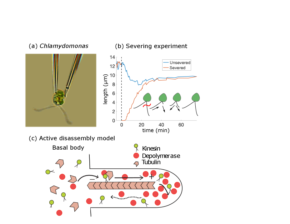
In [17], we proposed an active disassembly model for flagellar length regulation in Chlamydomonas based on physical first principles of flux balance (Figure 1(c)). By providing a mechanism for length-dependent disassembly, this model leads to simultaneous length control consistent with the length-equalization observed in severing experiments.
In this work, we consider the mathematical properties of the system of nonlinear ordinary differential equations that make up the active disassembly model. While it is well-known that in principle nonlinear equations may lead to behaviors such as finite time blow-up or oscillations, we show that these behaviors can be ruled out over a wide range of parameters. Moreover, we generalize the model to the case of arbitrary flagellar number, motivated by the olfactory sensory neurons which have on the order of 5–20 cilia per cell.
We show that these equations have a global asymptotically stable steady-state solution. To prove this, we find a Lyapunov function for the dynamics. The Lyapunov function also implies there are no limit cycles or periodic oscillations. Further, we construct a hybrid system to ensure that the flagellar lengths remain non-negative, and this yields regions of state space from which all trajectories contract to a single point on the boundary before flowing toward steady-state. We interpret these trajectories in light of existing experimental data. In addition, we provide alternate proofs of global asymptotic stability and the non-existence of periodic oscillations that do not rely on the construction of a Lyapunov function. We discuss how these results generalize to other situations.
By characterizing the mathematical properties of the active disassembly model, we aim to provide a strong foundation for subsequent applications and analysis of the model. In the Discussion, we note several open questions regarding the mathematical model and its application to organelle size control.
1 Active disassembly model of flagellar length control
As described in the Introduction, the process of IFT involves the transport of various biomolecules between the flagellar base and tip, and is believed to be closely linked with the dynamics of flagellar length. In the development of the mathematical model described next, we conceptually simplify this process by capturing only the essential biomolecular constituents for length control. In particular, we restrict attention to the tubulin that makes up the axoneme structure, the molecular motors that power transport along the axoneme, and the depolymerase conjectured to be necessary for length control. We assume that both assembly and disassembly are in continual competition so that the overall growth rate is the net result of these processes. Next, we describe the assembly and disassembly rates that give rise to differential equations for the flagellar lengths.
Let and denote the lengths of two flagella on a single Chlamydomonas organism at a particular time . The flagellum is composed of tubulin filaments, and we assume there is a total amount of tubulin available. The units of tubulin are given in microns, so that the pool size and flagellar lengths have the same units and the amount of free tubulin at the flagellar base is given by .
We assume there are a total number of anterograde molecular motors, of which a number are free in the basal pool while the others are undergoing IFT. In line with the pattern of motion found experimentally for kinesin [18], the motors move ballistically in the anterograde direction with velocity and diffusively in the retrograde direction with diffusion coefficient .
The injection flux of IFT particles into the flagella satisfies mass action kinetics, so that
| (1) |
There is a separation of timescales between the motion of IFT particles, which traverse the flagellum in several seconds, and the flagellar length dynamics, which varies over a timescale of several minutes [19]. As shown in Appendix A, upon combining (1) with conservation of protein number, this separation of timescales leads to a quasi-steady state approximation for the flux:
| (2) |
The flux represents the number of IFT particles injected per second into the flagella, and these particles are assumed to carry an amount of tubulin proportional to the free tubulin in the basal pool. Therefore, the overall speed of assembly is equal to , where is a proportionality constant that represents the fraction of tubulin arriving at the flagellar tip that is incorporated into the flagellum.
Disassembly is taken to be a linear function of the depolymerase concentration at the flagellar tip, i.e. each depolymerizing enzyme located near the flagellar tip removes a constant number of tubulin subunits per second. This implies that for the th flagellum for , the speed of disassembly is equal to , where and are the coefficients of the first-order Taylor series approximation. As explained in detail in Appendix A, this follows from the assumption that there is a depolymerase which has the same ballistic-to-diffusive pattern of motion as kinesin: the disassembly rate equals , where is the concentration of depolymerase at the flagellar tip.
Setting the growth rate to be the difference between assembly and disassembly speeds leads to a system of coupled nonlinear differential equations:
| (3) | ||||
| (4) |
where satisfies
| (5) |
1.1 Nondimensionalization
We next rewrite eqs. 3 and 4 in dimensionless form. In terms of the nondimensional length and nondimensional time as well as the dimensionless parameters , , , and , the system of equations eqs. 3 and 4 becomes
| (6) | |||
| (7) |
where the dimensionless flux satisfies
| (8) |
We interpret the dimensionless parameters as follows: is the ratio of disassembly and assembly rates, is the depolymerase activity level, is the ratio of the ballistic timescale of IFT transport to the injection timescale , and is an analogous ratio of the diffusive timescale to the injection timescale. (We could equivalently think of and as ratios of lengthscales related to the same physical processes.)
It is a straightforward calculation to verify that both flagella have the same steady-state length given by
| (9) |
1.2 Generalization to arbitrary flagellar number
Here we generalize the flagellar length control model to arbitrary . We are motivated by cells such as olfactory sensory neurons (OSN’s), which have on the order of a dozen cells, as we shall discuss later on in detail. In this case, the equations corresponding to eqs. 3, 4 and 5 become:
| (10) | ||||
| (11) |
To put the equations in dimensionless form, we follow the approach taken in the case above by introducing the dimensionless variables and as well as the dimensionless parameters , , , and . This leads to the following system, which generalizes eqs. 6, 7 and 8 above:
| (12) | ||||
| (13) |
As in the case , (12) leads to a unique fixed point with for with
| (14) |
which decays as as .
Note that, in the limit for fixed and , the dimensionless basal disassembly parameter satisfies . This is because the injection rate into any one flagellum, which goes as , becomes smaller and smaller in comparison to the -independent basal disassembly , resulting in steady-state lengths of zero beyond a critical value of . However, in the special case , one obtains flagella of progressively smaller but nonzero lengths as .
1.3 Ofactory sensory neuron cilia
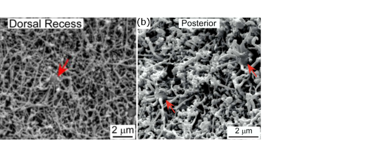
We next apply the active disassembly model to data on olfactory sensory neurons (OSN’s) from the mouse nasal septum. These cells each have on the order of 5–20 cilia, and the number depends on the cell’s location the within the dorsal zone. (The structures of cilia and flagella are the same and the terms may be used interchangeably.) In particular, it is reported in [20] that cells in the anterior region have cilia, whereas cells in the posterior region have cilia. Not only the cilia number but also the average lengths are location-dependent, with anterior cilia having lengths of µm and posterior cilia having shorter lengths of µm.
This data provides an opportunity to apply our model of length control to study the correlation between cilia number and length. Notably, it is not the case that posterior cells having fewer cilia tend to have longer cilia. Interpreting this data through the active disassembly model, which in the limit of large implies the steady-state lengths satisfy , this implies that cells in different regions have different tubulin pool sizes. Accordingly, we estimate the pool sizes of OSN’s in the anterior to be µm and for OSN’s in the posterior to be µm.
If we assume protein concentrations are held roughly constant across the dorsal zone, this means the pool size should scale with volume, and based on the spherical shape of OSN’s implies a scaling of . Plugging in the numbers above, the model predicts that , whereas direct measurement of the cell radii from published images of OSN’s yields a ratio of . As data is sparse, we use an available image from the dorsal recess to approximate the diameter of anterior OSN’s. See Figure 2, which shows how the OSN diameters are estimated using images from [20].
This analysis leads to several conclusions. First, the assumption of constant concentrations of ciliary proteins appears to be inconsistent with the variations of cilia length and number observed across the dorsal zone. This indicates that concentration gradients may be responsible for sustaining the different pool sizes predicted by the model. Interestingly, computing the ratio of cilia number yields , which suggests that cilia number scales with volume. The mechanism for this apparent scaling relation remains an open question.
2 Nonlinear behavior
Next, we turn to the mathematical analysis of the dynamical equations. To simplify notation, we drop tildes and use the dimensionless formulation for the remainder of the article. We will first consider the case of flagella, and later on show that the key results generalize to arbitrary flagellar number. The active disassembly model eqs. 6 and 7 is not a gradient system, i.e. it cannot be written as the gradient of an energy function . This is proven by contradiction. Suppose there is an energy function such that and . Then, by equality of mixed partials
| (15) |
i.e.
| (16) |
However, the left-hand side of the equality is equal to
| (17) |
whereas the right-hand side is equal to
| (18) |
Because , we have . Assuming , it follows that there is equality if and only if . We have thereby reached the contradiction since in general. It follows that no energy function exists.
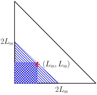
However, using a technique applicable to many nonlinear dynamical systems, we may construct a Lyapunov function to show that the steady state is globally asymptotically stable. First, we specify the subspace with over which the model is defined. Because we must have for the variables to have physical meaning as lengths, is contained within the first quadrant. Moreover, the sum of lengths cannot exceed the total pool size so that . To summarize, is defined to be the triangular region in the first quadrant bound by the lines , , and .
We define the deviations from steady-state and on and express the dynamics in terms of and :
| (19) | ||||
| (20) |
or equivalently
| (21) | ||||
| (22) |
By symmetry, the steady-state lengths and are equal. We denote the common steady-state length by . It is determined by setting the derivative equal to zero in (21) or (22), which yields the identity
| (23) |
where
| (24) |
(Eq. (23) yields a quadratic equation for , which has a unique positive root given by (9).)
We next use the steady-state relationship (23) to rewrite eqs. 21 and 22 in a different form. Before we proceed, we first note the identities given by
| (25) | ||||
| (26) |
where the first line follows from adding and subtracting and the second line follows from adding and subtracting . Plugging the above expressions into eqs. 21 and 22 and using the steady-state relation (23) yields
| (27) | ||||
| (28) |
Adding and subtracting the above equations yields
| (29) | ||||
| (30) |
It follows that
| (31) | ||||
| (32) |
where we have used for and
| (33) | ||||
| (34) |
Claim.
is a Lyapunov function on .
We first comment on some implications of the above claim before proceeding with its proof. It follows from the claim that there is a unique steady-state at which and that no limit cycles exist in .
Proof.
Since it is the sum of squared terms with positive factors, . It remains to show that with equality achieved only at the unique steady-state . Because the second term of has a non-positive derivative (by (32)), a sufficient condition for is that the right-hand side of (31) is negative away from the steady-state, i.e.
| (36) |
except when in which case it is zero. As we show next, in some cases (36) holds and the claim immediately follows. Later on, we show how, if (36) does not hold, we may use the second term of to obtain the desired result .
It follows from the steady-state condition (23) that
| (37) |
Therefore, the first term on the left-hand side of (36) may be rewritten as
| (38) |
To simplify the right-hand side of the above expression, we use the definition of the flux (8) to get
| (39) |
Note that
| (40) |
and moreover
| (41) |
Combining eqs. 38, 39, 40 and 41, for the left-hand side of (36) we have
| (42) |
To show the above expression is negative, we consider two cases. In the case , the term in parentheses on the right-hand side of (42) is a sum of squared terms multiplied by positive numbers. Therefore the right-hand side of (42) is negative.
In the case , we may bound the positive term by the negative terms in the right-hand side of (42) to show that the overall expression is negative. In this case, must reside in a triangular subset (the striped region in Fig. 3).
On this subset, if both and are negative, then
| (43) |
and moreover , so that
| (44) |
and since this term already appears in (42) with a minus sign it follows that the right-hand side of (42) is negative.
On the other hand, if and have opposite signs, then we must use a different bound. From the geometry of the relevant triangular subset , we have as before so that
| (45) |
From the condition that the flagella initially grow if they start at zero length, we have , and from the steady-state equation (23) it follows that . Therefore
| (46) |
It follows that is bounded above by , where is the right-hand side of (32). Therefore,
| (47) |
∎
Next, we consider whether is a trapping region closed to the dynamics. That is, we must consider whether any trajectories originating in may eventually leave . First, we show that no trajectories cross the boundary. To show that all trajectories move inward from this boundary, we calculate
| (48) |
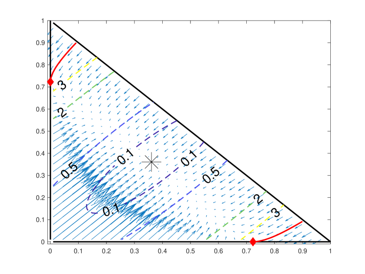
This proves that trajectories flow inward cannot leave across the boundary. See Figure 4 for an illustration of as well as the slope field and contours of .
In addition, for to be a trapping region, no trajectories should escape the first quadrant. In terms of , this means that no trajectories cross the axis on the interval , and no trajectories cross the axis on the interval . However, the model eqs. 6 and 7 does not satisfy this requirement. To the contrary,
| (49) |
and upon solving the quadratic equation resulting from one finds that there is a unique positive root
| (50) |
Therefore, to prevent trajectories that cross the -axis resulting in negative lengths, we construct a hybrid system by setting when on . This results in trajectories that flow down to the -axis, move horizontally according to this modified dynamics with until they reach , at which point they rejoin the full dynamics and move toward steady state. The dynamics are modified symmetrically to prevent trajectories from crossing the -axis as well.
To characterize the trapping region of the full dynamics, we therefore define the trajectory going backward in time from the point , as defined by
| (51) |
up until it hits the diagonal . We define another trajectory similarly as the one going backward in time from the point . The points from which the trajectories and originate are illustrated by red diamonds and the trajectories are shown as red curves in Fig. 4.
As a consequence of the modified dynamics, trajectories originating in the corner regions of phase space bounded by and consist of three distinct phases: first, there is flow down to the or -axis, followed next by horizontal or vertical motion to the point or , respectively, and finally leading to recovery by the full dynamics back to steady state. One interesting consequence of this behavior is its interpretation in the context of severing experiments. We find that the typical severing protocol, in which the two flagella first reach steady-state before severing takes place, does not lead to states within the corner region (purple trajectory in Fig. 5).
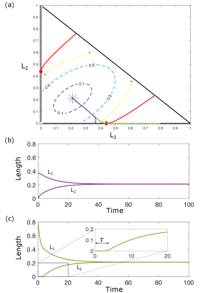
Fig. 5 shows a representative simulation of a severing experiment. The code used to generate this simulation and the corresponding figures is included in our open source code repository located at https://github.com/thomasgfai/StabilityFlagellarLengths.
If the system is initially out of steady-state, however, severing may result in a state outside the trapping region. This yields two phases of flow after severing: first, a horizontal flow to the accumulation point , and second a flow by the full dynamics to reach the global steady-state (green trajectory in Fig. 5). As shown in the inset of Fig. 5(c), this first phase of horizontal flow leads to an apparent delay in the response of the cut flagellum.
As mentioned above, the corner regions that lead to negative lengths in the original active disassembly model are not encountered in typical biological scenarios. One may nevertheless ask how a model derived from physical principles could lead to negative lengths. In our case, this behavior arises because of the basal disassembly rate that appears in the model, which implies a nonzero rate of disassembly even when the flagellum is very small. In the corner regions of the phase space, this basal term is greater than the rate of assembly because the tubulin pool is nearly depleted. This leads to a negative growth rate at zero length. Note that this issue does not arise in agent-based models in which each tubulin monomer is treated explicitly, since in that case disassembly only occurs when the flagellum contains at least one monomer. Within the ODE model, the modified dynamics ensure that disassembly only occurs when there are tubulin monomers remaining on the flagellum. Alternatively, one could rectify this issue by defining to be a step function of length that turns off once a flagellum is sufficiently small.
2.1 Nonexistence of Oscillations: Alternate Proof
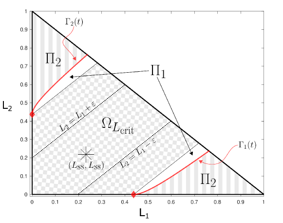
Recall that we have an invariant set on the domain by construction. In this section, we use an alternative approach to exclude oscillations using standard methods in dynamical systems. The proof will primarily focus on the region of containing the fixed point that is bounded by the lines :
where . An example of this domain is shown in Figure 6 for (checkerboard region). The boundary of for is shown using dotted lines, labeled . The smaller the value of , the thinner the domain will be. We will first show that is a trapping region (invariant set) for each arbitrarily small, by showing that the flows across the sections defined by the lines are always inward towards the fixed point . This condition is sufficient because we have already shown that flow along the relevant boundaries of point inwards, specifically, and for , and . To prove the non-existence of oscillations, we assume it exists and show that a portion of the oscillation must escape for some and can not return, which is a contradiction.
Claim.
is an invariant set.
In the ensuing proof, we show that the flows across the sections defined by the lines are always inward towards the fixed point . Combined with the inward flow along the boundaries of , this inward flow across the lines is sufficient to prove the claim.
Proof.
To show that the vector field points inwards for a given , we show that along and along . First, we plug in into the right hand side of eqs. 6 and 7 and take the difference :
Therefore, independent of the choice of . Inward flow along the lower boundary follows using the same argument. Thus, for each , the set is invariant.
We now proceed with a proof by contradiction. Suppose that there exists a periodic solution. Every oscillating solution must surround at least one fixed point (see index theory, [21]), and the only fixed point of this system exists within . Therefore, the oscillating solution surrounds the fixed point , and there exists some such that parts of the periodic solution lie outside of . (If an oscillating solution is fully contained within for some , to obtain we may simply reduce until parts of the periodic solution lie outside of .) It follows that solutions must exit , but this contradicts being an invariant set. ∎
2.2 Global Asymptotic Stability: Alternate Proof
Claim.
The fixed point is globally asymptotically stable in .
Proof.
We will consider three parts of the domain. First, for (Figure 6, checkerboard region), second, the region between and which we call (Figure 6, white region within ), and third, the region (Figure 6, striped region). The sets , , and are taken to be closed.
We begin our proof with and because they are the most straightforward. In , all solutions exit through one of the lines . This observation follows because there are no fixed points in and flows cannot cross the solution . In , we force all flows to exit through or by definition. Therefore, all flows originating in will enter the trapping region .
It remains to show asymptotic stability in . Note that our system is continuously differentiable on all of and therefore existence and uniqueness of solutions holds for all time. Before proceeding with the proof of asymptotic stability, we recall two basic definitions.
Definition 1.
The positive semiorbit is defined as the set
Definition 2.
The -limit set of a point , , is the set of those points for which there exists a sequence with , where is the flow of an autonomous ODE , and is an open subset of [22]. The omega-limit set for a trajectory is defined analogously.
In the case that all solutions are bounded, only certain types of -limit sets are possible. This is a consequence of the following theorem (Theorem 7.4.2 in [23]):
Theorem 1.
Let be a positive semiorbit contained in a compact subset of and suppose that contains only a finite number of equilibrium points. Then
-
1.
consists of a single point which is an equilibrium point of , and for an initial condition , as , or
-
2.
is a periodic orbit, or
-
3.
consists of a finite set of equilibrium points together with their connecting orbits. Each such orbit approaches an equilibrium point on and as .
This theorem, which follows from the Poincaré-Bendixson theorem, tells us that if a solution is trapped in a compact domain for all time, then a single equilibrium must be either a unique asymptotically stable point or a saddle-like point with at least one pair of connected unstable and stable manifolds. (The saddle-like observation follows by the third part of the theorem; a single equilibrium can also be stable in backwards time.)
Because we have eliminated periodic orbits in and shown that our stable fixed point is locally asymptotically stable and therefore cannot be saddle-like, we must have an asymptotically stable equilibrium point in . Finally, because all solutions in eventually reach the trapping region , is the globally asymptotically stable equilibrium point in . ∎
2.3 Generalization to organisms with flagella
Next, we prove global asymptotic stability in the case of arbitrary flagellar number by constructing a Lyapunov function, following similar logic to that used in the case. In the following, we once again drop the tildes for convenience. Define as before for and let
| (52) |
Claim.
is a Lyapunov function on .
Proof.
We first note that setting the derivative to zero in (12) yields the identify
| (53) |
where
| (54) |
Following the logic of the proof in the case results in the equations
| (55) | ||||
| (56) |
From the steady-state identify (53), we have
| (57) |
so that the first term on the right-hand side of (55) may be rewritten as
| (58) |
The expression above may be simplified further by using the definition of the flux to obtain
| (59) |
and noting that
| (60) |
Moreover, we may rewrite the first term on the right-hand side above by adding and subtracting to obtain
| (61) |
Combining eqs. 58, 59, 60 and 61 yields
| (62) |
The first three terms in parentheses on the right-hand side of (62) are clearly positive. The final term may be bounded according to
| (63) |
where the final inequality follows from , by (53) and the definition of , which asserts that the sum of lengths must not exceed the total pool size.
Note that the Lyapunov function we construct for general does not reduce to the Lyapunov function constructed previously in the case . There is an additional factor of two in the second term of . However, there is no inconsistency; the Lyapunov function is not unique. Still, the Lyapunov function constructed previously provides a tighter bound in the case , and we conjecture that the factor of two in the second term of the Lyapunov function in (52) is not essential.
3 Discussion
We have modified the active disassembly model originally proposed in [17] by constructing a hybrid system to ensure that the flagellar lengths remain positive for all time, regardless of the initial conditions. Further, we have used the method of Lyapunov functions (as well as the Poincaré-Bendixson Theorem) to prove the existence of an asymptotically stable steady-state. Although the Poincaré-Bendixson Theorem is limited to systems of two equations, the Lyapunov approach is shown to generalize to .
The Lyapunov function provides significant constraints on the possible dynamics, e.g. there can be no periodic cycles or finite time blow-up and solutions flow inextricably down the gradients of the Lyapunov function toward the unique steady-state. This highly-constrained solution space is a testable prediction of the active disassembly model.
Finally, we discuss aspects of length control in the case of a large number of organelles. Indeed, this is a biologically-relevant case given that single-cell organisms such as Paramecium cells swim using on the order of five thousand cilia [24]. Depending on which parameters are fixed in the limit , our dimensional analysis of the active disassembly model yields different limiting behaviors. A remarkable consequence of the model is that it provides a universal length-control mechanism regardless of organelle number, and an important next step would be to establish the limits of the model by testing its predictions on different organisms over a range of .
This generalization to arbitrary flagellar number reveals that while the active disassembly model was originally motivated by Chlamydomonas reinhardtii with its two flagella, it is universal in the sense that it achieves length control for any number of organelles. We have further explore the implications of this universal mechanism for controlling the sizes of large numbers of organelles by applying the model to study olfactory sensory neurons. The model provides possible explanations for scaling relations between cell size and flagellar length observed in the data.
An important caveat is that in organisms with more than two flagella, some of the assumptions of our model may need to be modified. For example, Giardia has eight flagella organized in four pairs, with each pair having a different steady-state length [25]. In order to represent length control in Giardia using the active disassembly model, the same overall modeling framework could be used with suitable modifications. For instance, each flagellar pair could be taken to have different parameters, such as the injection rate at the flagellar base, for example, or the tubulin and/or motor pools may be taken to be separate containing different amounts of protein for each of the four pairs.
4 Acknowledgments
We thank Ariel Amir and Te Cao for providing feedback on an early version of this manuscript. We further acknowledge useful discussions with Prathitha Kar, Lishibanya Mohapatra, and Jane Kondev, and Rosemary Challis for providing data on cilia lengths in olfactory sensory neurons. We acknowledge support under National Science Foundation grant DMS-1913093 (TGF) and National Institute of Health grant T32 NS007292 (YP).
Appendix A Flux derivation
Consider the lengths of two flagella and their evolution in time, which we denote by and . As stated in Section 1, we assume a total number of molecular motors and a total amount of tubulin .
We now derive the dynamical equations for the flagellar lengths, closely following [17]. Assembly occurs in two steps in our model, each of which follows the law of first-order chemical kinetics. First, tubulin aggregates on an IFT particle containing a single molecular motor. Second, the IFT particles are injected into the flagellum. The first step of protein aggregation on IFT particles results in particles carrying an amount of tubulin proportional to . In the second step, i.e. the injection of IFT particles at the flagellar base, the number of free molecular motors determines the injection rate via:
| (65) |
where is the rate constant of injection and the factor of one half is due to equal probabilities of injection into either flagellum.
Because the timescale of IFT (order of seconds) is fast compared to the timescale of changes in the flagellar lengths (order of minutes), we assume a quasi-steady state in which there is no accumulation of IFT particles along the flagellum. Therefore, the rate of injection equals the arrival flux of IFT particles to the flagellar tip.
The assembly rate is assumed proportional to this arrival flux times the average amount of tubulin carried by an IFT particle, resulting in
| (66) |
where is a constant of proportionality.
As mentioned above . In order to express in terms of the flagellar lengths, we must incorporate the detailed motion of proteins during IFT. While, as mentioned above, IFT particles including the motors and cargo move at constant speed in the anterograde direction, it has been shown that some IFT proteins such as kinesin motors diffuse in the retrograde direction back to the flagellar base [18]. We capture these different possibilities by letting and represent the numbers of motors undergoing ballistic and diffusive motion, respectively, on the th flagellum. By conservation of motor number, we have
| (67) |
We may express the ballistic flux on the th flagellum as the product of the concentration of motors moving ballistically in the anterograde direction times their speed:
| (68) |
where is the IFT speed in the anterograde direction.
On the other hand, To capture this diffusive motion, we let the concentration of diffusing particles on the th flagellum be for positions along the flagellum. If the diffusive flux is constant, then by Fick’s law so that the concentration will be a linear function of , and in particular
| (69) |
where we have used the fact that .
Assuming the flagellar base acts as a sink, we may apply the boundary condition to (69) and express the flux in terms of the number of diffusing motors:
| (70) |
and it follows that
| (71) |
Since by the quasi-steady state assumption, we drop the subscripts and denote the constant flux by . Plugging the expressions from eqs. 67, 68 and 70 into (66) yields
and upon solving for we obtain
| (72) |
Inserting this expression into (66) yields finally
| (73) |
where is given by (72).
For the disassembly rate, we assume there is both a basal rate of disassembly as well as an additional disassembly which depends on the concentration of depolymerase at the flagellar tip. For simplicity, we will assume that the depolymerase concentration at the th flagellum is proportional to the kinesin concentration . (As discussed in [17], this would be the case so long as the depolymerase follows the same pattern of ballistic anterograde to diffusive retrograde motion.) Therefore, we have
| (74) |
Subtracting the assembly and disassembly rates yields the following system of coupled nonlinear ODE’s:
| (75) | ||||
| (76) |
where is given by (72) above.
References
- [1] D. Zink, A. H. Fischer, J. A. Nickerson, Nuclear structure in cancer cells, Nature Reviews Cancer 4 (9) (2004) 677–687.
- [2] J. B. S. Haldane, On being the right size, Harper’s Magazine 152 (1926) 424–427.
- [3] W. F. Marshall, Cell geometry: How cells count and measure size, Annual Review of Biophysics 45 (2016) 49–64.
- [4] R. Milo, R. Phillips, Cell biology by the numbers, Garland Science, 2015.
- [5] K. A. Wemmer, W. F. Marshall, Flagellar length control in Chlamydomonas—a paradigm for organelle size regulation, International Review of Cytology 260 (2007) 175–212.
- [6] B. L. Gutman, K. K. Niyogi, Chlamydomonas and Arabidopsis. a dynamic duo, Plant Physiology 135 (2) (2004) 607–610.
- [7] R. E. Goldstein, Green algae as model organisms for biological fluid dynamics, Annual Review of Fluid Mechanics 47 (2015) 343–375.
- [8] P. A. Salomé, S. S. Merchant, A series of fortunate events: Introducing Chlamydomonas as a reference organism, The Plant Cell 31 (8) (2019) 1682–1707.
- [9] K. Y. Wan, G. Jékely, On the unity and diversity of cilia, Philosophical Transactions of the Royal Society B 375 (1792) (2020) 20190148.
- [10] R. L. Nguyen, L.-W. Tam, P. A. Lefebvre, The LF1 gene of Chlamydomonas reinhardtii encodes a novel protein required for flagellar length control, Genetics 169 (3) (2005) 1415–1424.
- [11] D. K. Khona, V. G. Rao, M. J. Motiwalla, P. S. Varma, A. R. Kashyap, K. Das, S. M. Shirolikar, L. Borde, J. A. Dharmadhikari, A. K. Dharmadhikari, et al., Anomalies in the motion dynamics of long-flagella mutants of Chlamydomonas reinhardtii, Journal of Biological Physics 39 (1) (2013) 1–14.
- [12] B. Morga, P. Bastin, Getting to the heart of intraflagellar transport using Trypanosoma and Chlamydomonas models: the strength is in their differences, Cilia 2 (1) (2013) 16.
- [13] K. G. Kozminksi, K. A. Johnson, P. Forscher, J. L. Rosenbaum, A motility in the eukaryotic flagellum unrelated to flagellar beating, Proceedings of the National Academy of Sciences 90 (12) (1993) 5519–5523.
- [14] J. M. Scholey, Intraflagellar transport, Annual Review of Cell and Developmental Biology 19 (1) (2003) 423–443.
- [15] J. L. Rosenbaum, J. E. Moulder, D. L. Ringo, Flagellar elongation and shortening in Chlamydomonas: the use of cycloheximide and colchicine to study the synthesis and assembly of flagellar proteins, The Journal of Cell Biology 41 (2) (1969) 600–619.
- [16] W. B. Ludington, L. Z. Shi, Q. Zhu, M. W. Berns, W. F. Marshall, Organelle size equalization by a constitutive process, Current Biology 22 (22) (2012) 2173–2179.
- [17] T. G. Fai, L. Mohapatra, P. Kar, J. Kondev, A. Amir, Length regulation of multiple flagella that self-assemble from a shared pool of components, eLife 8 (2019) e42599.
- [18] A. Chien, S. M. Shih, R. Bower, D. Tritschler, M. E. Porter, A. Yildiz, Dynamics of the IFT machinery at the ciliary tip, eLife 6 (2017) e28606.
- [19] N. L. Hendel, M. Thomson, W. F. Marshall, Diffusion as a ruler: modeling kinesin diffusion as a length sensor for intraflagellar transport, Biophysical Journal 114 (3) (2018) 663–674.
- [20] R. C. Challis, H. Tian, J. Wang, J. He, J. Jiang, X. Chen, W. Yin, T. Connelly, L. Ma, C. R. Yu, et al., An olfactory cilia pattern in the mammalian nose ensures high sensitivity to odors, Current Biology 25 (19) (2015) 2503–2512.
- [21] J. Guckenheimer, P. Holmes, Local bifurcations, in: Nonlinear oscillations, dynamical systems, and bifurcations of vector fields, Springer, 1983, pp. 117–165.
- [22] G. Teschl, Ordinary differential equations and dynamical systems, Vol. 140, American Mathematical Soc., 2012.
- [23] N. Lebovitz, Ordinary differential equations, Cengage Learning, 2019.
- [24] A. Funfak, C. Fisch, H. T. Abdel Motaal, J. Diener, L. Combettes, C. N. Baroud, P. Dupuis-Williams, Paramecium swimming and ciliary beating patterns: a study on four RNA interference mutations, Integrative Biology 7 (1) (2015) 90–100.
- [25] S. G. McInally, S. C. Dawson, Eight unique basal bodies in the multi-flagellated diplomonad Giardia lamblia, Cilia 5 (1) (2016) 21.