Global solutions with infinitely many blowups in a mean-field neural network

In this work, we consider idealized neural-network models called delayed Poissonian mean-field (dPMF) models introduced in [22]. These dPMF models are variations of classical mean-field models [5, 4, 7], whose dynamics are also prone to blowups. From a modeling perspective, blowups correspond to the occurrence of synchronous, macroscopic spiking events in a neural network. Understanding the emergence of these synchronous events is of interest for studying the maintenance of precise temporal information in neural networks [19, 15, 3]. However, blowups resist direct analytical treatment in classical mean-field models [10, 9, 13, 18, 17]. This observation is the primary motivation justifying the introduction of dPMF dynamics, whose blowups prove analytically tractable.

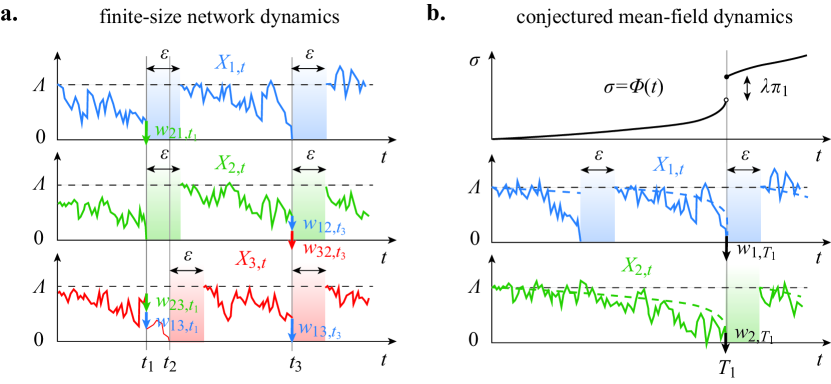
In [22], we conjectured dPMF dynamics as the mean-field limit of finite-size particle systems with singular interactions (see Fig. 1). In a finite-size system of $N$ particles, each particle $i$, $1\leq i\leq N$, represents a neuron with time-dependent state variable $X_{N,i,t}$. These state variables evolve jointly according to a $\mathbbm{R}^{N}$-valued continuous-time process $t\mapsto\{X_{N,i,t}\}_{1\leq i\leq N}$. Specifically, the network dynamics is parametrized by the drift value $\nu>0$, the refractory period $\epsilon>0$, and the interaction parameter $\lambda>0$ as follows: $(i)$ Whenever a process $X_{N,i,t}$ hits the spiking boundary at zero, it instantaneously enters its inactive refractory state. $(ii)$ At the same time, all the other active processes $X_{N,j,t}$ (which are not in the inactive refractory state) are respectively updated by amounts $-w_{N,ij,t}$, where $w_{N,ij,t}$ is independently drawn from a normal law with mean and variance equal to $\lambda/N$. $(iii)$ After an inactive (refractory) period of duration $\epsilon>0$, the process $X_{N,i,t}$ restarts its autonomous stochastic dynamics from the reset state $\Lambda>0$. $(iv)$ In between spiking/interaction times, the autonomous dynamics of active processes follow independent drifted Wiener processes with negative drift $-\nu$. Correspondingly, an initial condition for the network is specified by the starting values of the active processes, i.e., $X_{N,i,0}>0$ if $i$ is active, and the last inactivation time of the inactive processes, i.e., $-\epsilon\leq\rho_{i,0}\leq 0$, if $i$ is inactive. Following the above definition, the finite-size versions of dPMF dynamics exhibit two key features (see Fig. 1): $(1)$ recurrent interactions implement self-excitation whose strength is quantified by the interaction parameter $\lambda$; $(2)$ owing to the post-spiking refractory period $\epsilon>0$, individual neuronal processes follow delayed dynamics. Parenthetically, the inclusion of a negative drift $\nu$ is necessary to ensure that neurons will spike in finite time, independent of the initial conditions and of the coupling strength.

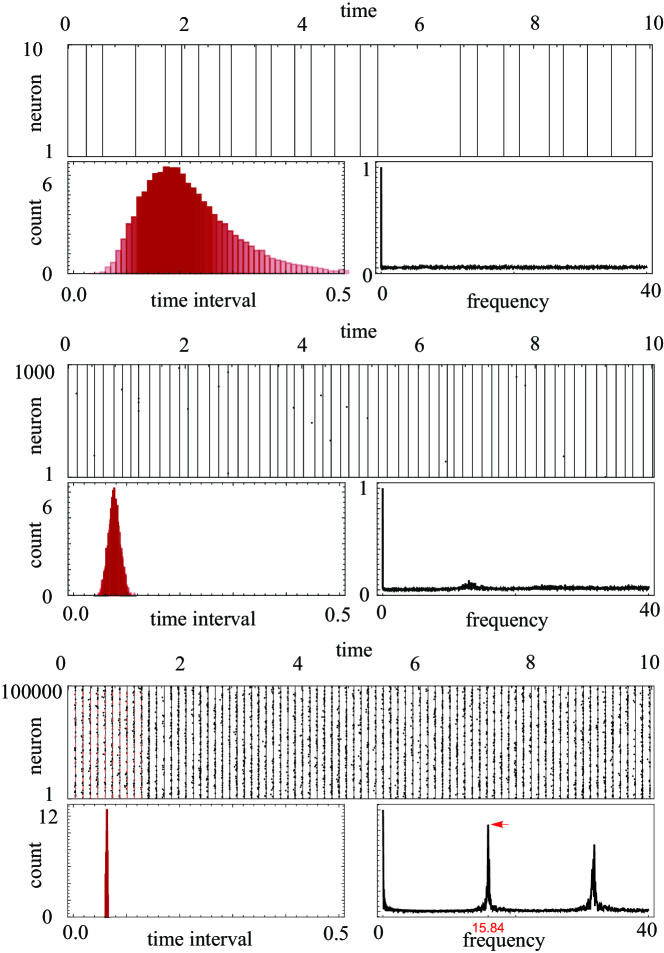
By analogy with [7, 8], dPMF dynamics are deduced from finite-size ones by conjecturing propagation of chaos in the infinite-size limit $N\to\infty$, which is supported by numerical simulations (see Fig. 2). The propagation of chaos states that for exchangeable initial conditions, the processes $X_{N,i,t}$, $1\leq i\leq N$, become i.i.d. in the limit of infinite-size networks $N\to\infty$, so that each individual process follows a mean-field dynamics [21]. For exchangeable initial conditions, a representative dPMF process $X_{t}=\lim_{N\to\infty}X_{N,i,t}$ is governed by the deterministic cumulative drift $\Phi$ that amalgamates the contribution of the autonomous drift $-\nu$ and the mean-field contribution of neuronal interactions via $\lambda$. Specifically, we have $\Phi(t)=\nu t+\lambda\mathbb{E}\left[M_{t}\right]$, where the process $M_{t}$ counts the successive first-passage times of the representative process $X_{t}$ to the zero spiking threshold. Such a process is defined as

with initial conditions bearing on $X_{0}$ or $\rho_{0}$ depending on the representative process being initially active or inactive. We will later specify such initial conditions in detail. Note that in the above definition, the first-passage times $\rho_{n}$, $n\geq 1$, denote successive inactivation times, whereas $r_{n}=\rho_{n}+\epsilon$, $n>0$, denotes the corresponding sequence of reset times. For mediating all interactions, the function $t\mapsto\mathbb{E}\left[M_{t}\right]$ plays a central role in our analysis. We denote this function by $F$ and observe that $F$ is defined as an increasing càdlàg function. Remember that a function is said to be càdlàg if it is right-continuous with left limits. Then, the hallmark of dPMF dynamics is that the drift $\Phi$ impacts the representative neuron stochastically via a process $Z_{t}=\Phi(t)+W_{\Phi(t)}$, where $W$ is a canonical, driving Wiener process. Accordingly, dPMF dynamics are referred to as Poissonian because the process $Z_{t}$ represents the diffusive limit of a Poisson counting process with $\mathbb{E}\left[Z_{t}\right]=\mathbb{V}\left[Z_{t}\right]$ for all $t\geq 0$. With these conventions, the stochastic dPMF dynamics of a representative process is given by

The above equation fully defines dPMF dynamics: The integral term indicates that when the neuron is active, for $X_{t}>0$, its state evolves according to the Poissonian diffusion process $Z_{t}$. The delayed term indicates that after hitting the spiking boundary at zero at time $\tau$, the process remains inactive until it resets at $\Lambda$ after a duration $\epsilon$: $X_{t}=0$ for $\tau\leq t<\tau+\epsilon$.

Because of their self-exciting nature, dPMF dynamics are prone to blowups/synchronous events for large enough interaction parameter and/or for initial conditions that are concentrated near the zero spiking boundary. Blowups occur at those times when $f$, the instantaneous spiking rate of a representative neuron, diverges. Formally, the firing rate $f$ is defined in the distribution sense as the Radon-Nikodym derivative of $F$ with respect to the Lebesgue measure: $f=\mathrm{d}F/\mathrm{d}t$. Then, assuming $f$ to be finite in the left vicinity of $T_{1}$, $T_{1}$ is a blowup time if $\lim_{t\to T_{1}^{-}}f(t)=\infty$. In turn, synchronous events occur at those times $T_{1}$ for which a finite fraction of processes spikes simultaneously or equivalently, for which a representative neuron spikes with nonzero probability: $\pi_{1}=\mathbb{P}\left[X_{T_{1}}=0\right]>0$. Formally, this corresponds to $F$ admitting a jump discontinuity at $T_{1}$ so that $F(T_{1})-F(T_{1}^{-})=\lambda\pi_{1}$.

The main interest of considering dPMF dynamics is that blowups and synchronous events are analytically tractable under some reasonable restrictions about the initial conditions. Specifically, denoting by $\mathcal{M}(I)$ the set of positive measure on an interval $I\subset\mathbbm{R}$, we assume as in [22] that:

The above initial conditions guarantee that there exists a dPMF dynamics locally solving (2) and that this dynamics is initially smooth in the sense that $F$ is an infinitely differentiable function in the right vicinity of zero. Such a smooth solution can be maximally continued on a possibly infinite interval $[0,T_{1})$, where $T_{1}$ marks the occurrence of the first blowup. In [22], we show that for all $0<t<T_{1}$, the density $x\mapsto p(x,t)=\mathbb{P}\left[X_{t}\in\mathrm{d}x\,|X_{t}>0\right]/\mathrm{d}x$ is smooth in the right vicinity of zero with $\lim_{x\to 0^{+}}p(x)=0$ and $\lim_{x\to 0^{+}}\partial_{x}p(t,x)/2<1/\lambda$. As the later limits are always well defined and finite, we will simply refer to their values as $p(0)$ and $\partial_{x}p(t,0)/2$ for conciseness. With this in mind, we show in [22] that for all $0<t<T_{1}$, the instantaneous spiking rate is given by

This leads to introducing the following criterion for first-blowup times:

The above criterion only bears on the local divergence of the firing rate $f$ and is silent about the possible occurrence of a synchronous event. To further characterize blowups, we introduce in [22] the so-called full-blowup criterion:

The full-blowup criterion, which generically holds with respect to the choice of initial conditions, allowed us to characterize blowups in dPMF dynamics as follows:

Thus, for generic initial conditions, blowups correspond to left Hölder singularity of exponent $1/2$ in the cumulative function $F$, followed by a jump discontinuity whose size $\lambda\pi_{1}$ can be determined as the solution of the self-consistent problem (3). In [22], we show that the latter problem directly follows from the requirement of conservation of probability during blowups.

Unfortunately, the blowup analysis of [22] is only local in the sense that it allows one to resolve a single blowup for generic initial conditions. However, this local analysis provides one with natural blowup exit conditions. In principle, these blowup exit conditions can also serve as initial conditions to analyze the next blowup, if any. Numerical simulations suggest that for large enough interaction parameters $\lambda>\Lambda$, explosive solutions exhibit repeated blowup episodes at regular time intervals (see Fig. 2). Following on this observation, the first goal of this work is to extend the analysis of [22] to show the existence of global dPMF solutions that are defined over the entire half-line $\mathbbm{R}^{+}$ and that exhibit a countable infinity of blowups. This program involves proving that for large enough interaction parameters, iteratively applying the blowup analysis of [22] produces synchronous events with sizes that remain bounded away from zero, at time intervals that also remain bounded away from zero. Moreover, the blowup analysis of [22] is only concerned with dPMF dynamics for positive refractory period $\epsilon>0$. With positive refractory period $\epsilon>0$, explosive dPMF dynamics are always well posed but at the analytical cost of being determined as delayed dynamics. For small enough $\epsilon>0$, we do not expect the refractory period to impact dPMF dynamics, except for ensuring their well-posedness in the presence of blowups. This suggests defining explosive Poissonian mean-field (PMF) dynamics in the absence of a refractory period as the limit dPMF dynamics obtained when $\epsilon\to 0^{+}$. Accordingly, the second goal of this work is to prove the existence and uniqueness of such limit dPMF dynamics. This will only be possible for large enough interaction parameters, when global dPMF dynamics sustain isolated blowups for small enough $\epsilon>0$. PMF dynamics with zero refractory period $\epsilon=0$ are of interest for analysis as their blowups can be resolved just as for $\epsilon>0$, whereas their inter-blowup dynamics are nondelayed.

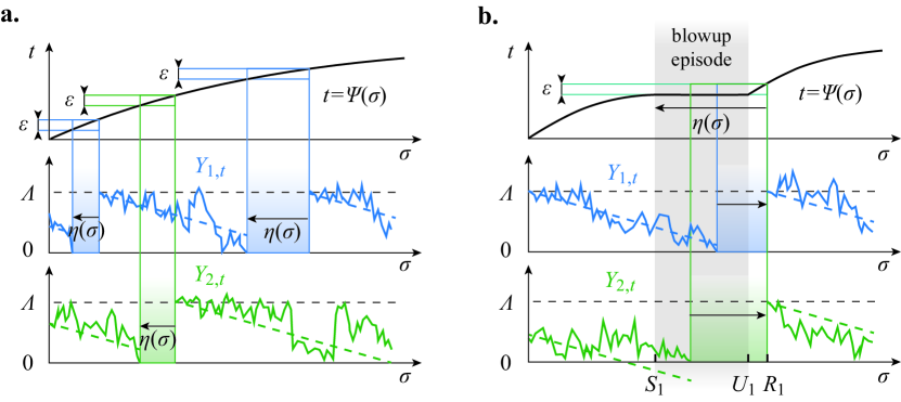
In [22], we analytically characterized blowup generation in dPMF dynamics by mapping the original time-homogenous, nonlinear dynamics onto a time-inhomogeneous, linear dynamics (see Fig. 3). Such a mapping is operated by considering the cumulative drift $\Phi$ as an implicitly defined time-change function

which is only assumed to be a càdlàg increasing function. Due to the Poisson-like attributes of the neuronal drives, the time change $\Phi$ parametrizes the dPMF dynamics of a representative process as $X_{t}=Y_{\Phi(t)}$, where the time-changed dynamics $Y_{\sigma}$ obeys a linear, noninteracting dynamics. The latter dynamics is that of a Wiener process absorbed at zero, with constant negative unit drift and with reset at $\Lambda$, but with time-inhomogeneous refractory period specified via a $\Phi$-dependent, backward-delay function $\sigma\mapsto\eta[\Phi](\sigma)$ (see Fig. 3). Independent of the presence of blowups, the functional dependence of $\eta$ on the time change $\Phi$ is given by

where $\Psi=\Phi^{-1}$ refers to the inverse of the strictly increasing time change $\Phi$. Given a backward-delay function $\eta$, the transition kernel of the process $Y_{\sigma}$ denoted by $(\sigma,x)\mapsto q(\sigma,x)=\mathrm{d}\mathbb{P}\left[Y_{\sigma}\in\mathrm{d}x\,|\,Y_{\sigma}>0\right]/\mathrm{d}x$ satisfies the time-changed PDE problem

with absorbing and conservation conditions respectively given by

In equations (6) and (7), $G$ denotes the $\eta$-dependent cumulative flux of $Y_{\sigma}$ through the zero threshold. By definition of the time change $\Phi$, which is such that $X_{t}=Y_{\Phi(t)}$, $G$ is related to the cumulative flux $F$ via $F=G\circ\Phi$. A key result of [22] is that as long as the delay function $\eta$ remains bounded, the PDE problem defined by (6) and (7) admits a unique solution parametrized by an unconditionally smooth cumulative function $G=G[\eta]$. This result holds even in the presence of blowups for the time-changed versions of the initial conditions given in Assumption 1. These time-changed initial conditions are specified as follows:

In light of (12), the cumulative function $G=G[\Phi]$ actually depends on $\Phi$ via $\eta=\eta[\Phi]$. This realization allows one to interpret the implicit definition of $\Phi$ given in (4) as a self-consistent equation for admissible time changes:

In [22], we show that such an interpretation specifies $\Phi$ as the solution of a certain fixed-point problem. This fixed-point problem turns out to be most conveniently formulated in term of the inverse time change $\Psi=\Phi^{-1}$, assumed to be a continuous, nondecreasing function. Given an inverse time change $\Psi$, the time change $\Phi$ can be recovered as the right-continuous inverse of $\Psi$. In the time-changed picture, blowups happen if the inverse time change $\Psi$ becomes locally flat and a synchronous event happens if $\Psi$ remains flat for a finite amount of time. Informally, flat sections of $\Psi$ unfold blowups by freezing time in the original coordinate $t$, while allowing time to pass in the time-changed coordinate $\sigma$. This unfolding of blowups in the time-changed picture is the key to analytically resolve blowups in dPMF dynamics. Concretely, this amounts to showing the existence and uniqueness of solutions to the following fixed-point problem:

In [22], we further showed that the cumulative flux $G[\eta]$, introduced in the PDE problem defined by equations (6) and (7), is most conveniently characterized in terms of an integral equation obtained via renewal analysis:

Definitions 1.3 and 1.4 fully specify the dPMF fixed-point problem in the time-change picture. In this time-changed picture, the occurrence of a (first) blowup involves two distinct times: the blowup trigger time $S_{1}$ and the blowup exit time $U_{1}$, so that a synchronous event of size $\pi_{1}$ corresponds to $\Psi$ remaining flat on $[S_{1},U_{1})$ with $S_{1}=U_{1}+\lambda\pi_{1}$ (see Fig. 4). The definition of the blowup trigger time $S_{1}$ directly follows from Proposition 1.1, which can be recast in the time-changed picture as:

In turn, the full-blowup assumption 2 admits a more natural but equivalent formulation in the time-changed picture:

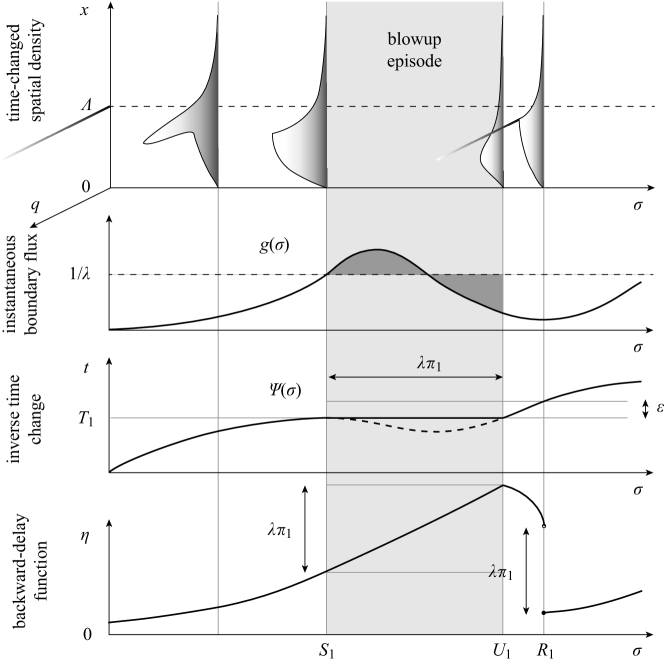
The above formulation of the full-blowup assumption is natural in view of the fixed-point problem 1.3. Indeed, such an assumption implies that the function $\sigma\mapsto\sigma-\lambda G(\sigma)$ becomes decreasing on a finite interval to the left of $S_{1}$. Thus, as a solution to the fixed-point problem (11), $\Psi$ must remain flat on a nonempty maximum interval $[S_{1},U_{1})$, which corresponds to a synchronous event of size $\pi_{1}=(S_{1}-U_{1})/\lambda$ (see Fig. 4). Incidentally, this observation sheds light on Definition 1.1 characterizing full blowups. During a full blowup episode, $\Psi$ remains flat so that the backward-delay function is constant on $[S_{1},U_{1})$. As a result, the renewal-type integral term in (13) vanishes and $G$ is revealed as the cumulative flux of a linear time-changed dynamics $Y_{\sigma}$, but without birth term due to reset. This amounts to stopping the clock for the original time coordinate $t$, while letting the clock run in the changed coordinate $\sigma$. Such a stoppage can only be maintained until $\Psi$ exceeds its blowup trigger value $\Psi(S_{1})$ (see Fig. 4), justifying the definition of blowup exit times $U_{1}$ as:

The above definition of the blowup exit time is consistent with the characterization of the blowup size $\pi_{1}$ given in (3). Indeed, one can check that

Then, introducing the reduced variable $p=(\sigma-S_{1})/\lambda$, we consistently have

where the last equality follows from the fact that the process $Y_{\sigma}$ does not reset on $[S_{1},U_{1})$. For nonzero vanishing period $\epsilon>0$, the processes that inactivate during a blowup episode reset after a period of duration $\epsilon$ elapses in original time coordinate. Thus, the reset time of a representative process $R_{1}$ shall satisfy $\Psi(R_{1})=\Psi(S_{1})+\epsilon$. The latter relation uniquely specifies $R_{1}$ if $\Phi=\Psi^{-1}$ is continuous in $T_{1}+\epsilon=\Psi(S_{1})+\epsilon$, which holds true if no blowup happens in $T_{1}+\epsilon$ (see Fig. 4). Following on [22], without any continuity assumption, the blowup reset time $R_{1}$ is generally defined as the leftmost solution of $\Psi(R_{1})=\Psi(S_{1})+\epsilon$:

The definitions of the blowup trigger time $S_{1}$, the exit time $U_{1}$, and the reset time $R_{1}$ illuminate how the time-changed process $Y_{\sigma}$ resolves a blowup episode by alternating two types of dynamics (see Fig. 4). Before a full blowup, the process $Y_{\sigma}$ follows a linear diffusion with absorption in zero and resets at $\Lambda$. These resets occur with time-inhomogeneous delays, which depends on the inverse time change $\Psi$. At the blowup onset $S_{1}$, $\Psi$ becomes locally flat, indicating that the original time $t=\Psi(\sigma)$ freezes, thereby stalling resets. As a result, after the blowup onset in $S_{1}$, the dynamics of $Y_{\sigma}$ remains that of an absorbed linear diffusion but without resets. Such a dynamics persists until a self-consistent blowup exit condition is met in $S_{1}+\lambda\pi_{1}$. This condition states that it must take $\lambda\pi_{1}$ time-changed units for a fraction $\pi_{1}$ of processes to inactivate during a blowup episode. Finally, the original time $t=\Psi(\sigma)$ resume flowing past $U_{1}$ and the inactivated fraction $\pi_{1}$ is reset at $\Lambda$ at time $R_{1}$. Importantly, observe that the time-change process $Y_{\sigma}$ always behaves regularly in the sense that $G$ remains a smooth function throughout the blowup episode.

In principle, dPMF dynamics could be continued past a blowup episode, and possibly even extended to the whole half-line $\mathbbm{R}^{+}$. Simulating the particle systems conjectured to approximate dPMF dynamics suggests that these dynamics can sustain repeated synchronization events over the whole half-line $\mathbbm{R}^{+}$ (see Fig. 2). This leads to conjecture the existence of solutions $\Psi$ globally defined on $\mathbbm{R}^{+}$ with a countable infinity of blowup episodes with associated sequence of blowup times $\{S_{k},U_{k},R_{k}\}_{k\in\mathbbm{N}}$. Extending results from [22] to show the existence of such global solutions requires showing:

• •

  Unconditional explosiveness: $(i)$ the so-called non-false-start exit condition $\partial_{\sigma}q(U_{k},0)/2<1/\lambda$ and $(ii)$ the full-blowup condition $\partial^{2}_{\sigma}\Psi(S_{k}^{-})<0$ are satisfied for all blowup episodes, not just for the first one.

• •

  Full-time domain: the blowup times $T_{k}=\Psi(S_{k})=\Psi(U_{k})$ do not have an accumulation point, i.e., $\lim_{k\to\infty}T_{k}=\infty$, which means that the explosive solution is defined over the whole half-line $\mathbbm{R}^{+}$.

The main difficulties in establishing the two above properties is that blowup times may not be well ordered, i.e., $R_{k}>S_{k+1}$ for some $k>0$ and that blowup sizes $\pi_{k}$ may exhibit vanishing sizes: $\lim_{k\to\infty}\pi_{k}=0$. However, one can exclude these possibilities in the strong interaction regime $\lambda\gg\Lambda$, for which the stable repetition of synchronization events can be understood intuitively:

$(i)$ Consider an initial condition of the form $q_{0}=\pi_{0}\delta_{\Lambda}$ with $\pi_{0}=1$, which corresponds to a full reset at time $R_{0}=0$ and which satisfies Assumption 1. For a full blowup to occur next, the post-reset flux $g$ needs to satisfy the full-blowup Assumption 3 at some trigger time $S_{1}$, where we must have $g(S_{1})=1/\lambda$ and $\partial_{\sigma}g(S_{1})>0$. For large enough $\lambda$, we expect this flux $g$ to be primarily due to processes that do not reset more than once on $[0,S_{1}]$. In other words, we have $g(\sigma)\simeq h(\sigma,\Lambda)$, where $h(\cdot,\Lambda)$ denotes the first-passage density of a Wiener process started at $\Lambda$ with unit negative drift and with a zero boundary. The function $h(\cdot,\Lambda)$ is known to be a strictly increasing convex function on some nonempty interval $[0,\sigma^{\dagger})$ with $h(0,\Lambda)=0$. Thus, choosing a large enough $\lambda>\Lambda$ guarantees that the full-blowup Assumption 3 will be met at some finite time $S_{1}>0$ with $S_{1}<\sigma^{\dagger}$. One can check the scaling $S_{1}\propto 1/\ln\lambda$, so that the fraction of inactive processes at trigger time $S_{1}$, denoted $P(S_{1})$, can be made arbitrarily small for large enough $\lambda$. Actually, provided the refractory period is such that $\epsilon=O(1/\lambda)$, one can find an upper bound for $P(S_{1})$ of the form $O(1/\lambda)$.

$(ii)$ Past the trigger time $S_{1}$, a fraction $1-P(S_{1})$ of processes are susceptible to synchronize during the blowup episode. It turns out that the actual size of the blowup $\pi_{1}<1-P(S_{1})$ can be made arbitrary close to $1-P(S_{1})$ for large enough $\lambda$. Again, this is because we still have $g(\sigma)\simeq h(\sigma,\Lambda)$ past the trigger time $S_{1}$, which satisfies $S_{1}<\sigma^{\dagger}$. This observation, together with the monotonicity properties of $h(\cdot,\Lambda)$, implies that $g(\sigma)>1/\lambda$ on $[\sigma^{\dagger},\sigma^{\star}]$, where $\sigma^{\star}$ is the unique maximizer of $h(\cdot,\Lambda)$. This means that the blowup episode includes at least the nonempty time interval $[\sigma^{\dagger},\sigma^{\star}]$, during which at least a fraction $\Delta_{H}=\int_{\sigma^{\dagger}}^{\sigma^{\star}}h(\sigma,\Lambda)\mathrm{d}\sigma>0$ synchronizes. Thus, we must have $\pi_{1}\geq\Delta_{H}>0$, so that the duration of the blowup $\lambda\pi_{1}\geq\lambda\Delta_{H}$ can be made arbitrary long for large enough $\lambda$. The key is then to observe that the tail behavior of $h(\cdot,\Lambda)$ indicates that inactivation during blowup asymptotically happens with hazard rate $1/2$ for large times. This observation allows one to deduce an exponential lower bound for the blowup size of the form, e.g., $\pi_{1}\geq\big{(}1-P(S_{1})\big{)}\big{(}1-O(e^{-\lambda\Delta_{H}/4})\big{)}>1/2$.

$(iii)$ Altogether, less than a fraction $1-\pi_{1}\leq O(1/\lambda)$ of processes survive the blowup at exit time $U_{1}=S_{1}+\lambda\pi_{1}$ with $\pi_{1}>1/2$. The distribution of these surviving processes is such that $\partial_{x}q(U_{1},0)/2\simeq h(U_{1},\Lambda)\leq O(e^{-U_{1}/2})=O(e^{-\lambda/4})<1/\lambda$ for large enough $\lambda$ so that the no-false-start Assumption 1 can be met for large enough $\lambda>\Lambda$. Moreover, we expect the fraction of surviving processes at $U_{1}$, i.e., $\|q(U_{1},\cdot)\|_{1}$, to be so small that they cannot trigger a blowup alone. In other words, the assumption of well-ordered blowups holds: the fraction of inactivated processes $\pi_{1}$ must reset at some time $R_{1}>U_{1}$ before any subsequent blowup can occur. Then, choosing $\pi_{1}=1-O(1/\lambda)$ close enough to one ensures that $g$ remains primarily shaped by those processes that reset at time $R_{1}$, so that $g(\sigma)\simeq\pi_{1}h(\sigma-R_{1},\Lambda)$. In turn, if the well-ordered property of blowups holds, we can apply $(i)$ anew but starting from $R_{1}$ with a controlled probability mass $\pi_{1}$, rather than the full mass $\pi_{0}=1$.

$(iv)$ To prove the well ordered property of blowups, one has to establish some a priori bounds about the boundary flux $g$ with respect to the $L_{1}$ norm $\|q(U_{1},\cdot)\|_{1}$. Establishing such a priori bounds requires to restrict the set of considered initial conditions to the so-called set of natural initial conditions. In a nutshell, these are those—not necessarily normalized—initial distributions such that all the active and inactive processes at the starting time have been reset at $\Lambda$ at some point in the past. For bearing on processes started away from zero at $\Lambda$, natural initial conditions cannot lead to large transient variations in boundary fluxes. As a result, one can show that in the absence of reset, $|g|$ and $|\partial_{\sigma}g|$ are uniformly upper bounded by $O(\|q(U_{1},\cdot)\|_{1})$. Then, the well-ordered property of blowups follows from showing that $|g|=O(\|q(U_{1},\cdot)\|_{1})<1/\lambda$ in the absence of the blowup reset. This requires that one has at least that $\|q(U_{1},\cdot)\|_{1}=O(1/\lambda)$, consistent with the fact that $\|q(U_{1},\cdot)\|_{1}\leq 1-\pi_{1}=O(1/\lambda)$. but not precise enough to conclude without explicit knowledge of the bounding coefficients..

$(v)$ Establishing that the no-false-start condition (Assumption 1), the full-blow up condition (Assumption 2), and the well ordered condition can be all met requires to estimate coefficients in the various $\lambda$-dependent bounds at play. Then, the strategy is to use these explicit bounds to show that given a large enough $\lambda>\Lambda$, there exists a threshold mass $\Delta_{\pi}$, $1/2<\Delta_{\pi}<1$, such that for all blowups of size $\pi_{1}\geq\Delta_{\pi}$, the next full blowup also satisfies $\pi_{2}>\Delta_{\pi}$. From there, a direct induction argument on the number of blowups shows that there is a unique inverse time change $\Psi:\mathbbm{R}^{+}\mapsto\mathbbm{R}^{+}$ dynamics as long as the initial mass $\pi_{0}\geq\Delta_{\pi}$. The fact that the domain of $\Psi$ is the full half-line $\mathbbm{R}^{+}$ follows from $\Psi$ having a countable infinity of blowup with size at least $\Delta_{\pi}>1/2$. The fact that the domain of $\Phi=\Psi^{-1}$ is also the full half-line $\mathbbm{R}^{+}$ follows from the fact that well ordered blowups must be separated by the duration of the nonzero refractory period $\epsilon>0$.

Making the arguments above rigorous leads to our first main result:

In the following, we prove an equivalent version of the above theorem for the time-changed dynamics, i.e., Theorem 3.2. The proof of Theorem 3.2 only relies on a few properties of the smooth first-passage density function $h(\cdot,\Lambda)$, which plays the key role throughout this analysis. Although we do not refer to these properties explicitly in the proof, we list them as follows:

Given some large enough Dirac-delta mass $\pi_{k}$ at reset time $R_{k}$, Property 1 ensures that a full blowup occurs for large enough $\lambda$ at trigger time $S_{k+1}>R_{k}$ and with blowup size $\pi_{k+1}$ lower bounded by some constant $\Delta_{H}$. This corresponds to the “ignition” phase of the blowup. Given that $\pi_{k+1}\geq\Delta_{H}$, Property 2 ensures that an exponentially small fraction of processes survives the blowup and that this fraction cannot lead to a subsequent blowup without reset, i.e., reignition. This corresponds to the “combustion” phase of the blowup. A potentially useful consequence of the above observations is that we expect our blowup analysis to extend to more generic diffusion processes. Indeed, the existence and uniqueness of explosive dPMF dynamics shall hold for all dynamics derived from autonomous diffusion processes whose first-passage time to a constant level has smooth densities satisfying Property 1 and 2. This class of diffusion processes includes the Ornstein-Uhlenbeck process, which forms the basis of a widely used class of models in computational neuroscience, called leaky integrate-and-fire neurons [16, 6].

In stating Theorem 1.8, we do note give a precise criterion for how to jointly choose the interaction parameter $\lambda>\Lambda$, the refractory period $\epsilon>0$, and the initial mass $\pi_{0}$ to yield explosive dPMF dynamics. This is because the precise criterion given in the proof of Theorem 1.8 is not tight, our main goal being to establish existence and uniqueness of global solution in the large interaction regime. Actually, we expect explosive dPMF dynamics to arise as soon as $\lambda>\Lambda$ for small $\epsilon\geq 0$ and we expect this emergence to be essentially independent of the size of the initial mass $\pi_{0}$. One can see the latter point by considering the limit case of PMF dynamics with zero refractory period in the time change picture. In the absence of blowups, plugging $\epsilon=0$ in Definition 1.3 yields valid, nondelayed dynamics with explicitly known instantaneous boundary flux $g$ via renewal analysis [1]. Moreover, classical arguments from renewal analysis show that $g$ is analytic away from zero and that $\lim_{\sigma\to\infty}g(\sigma)=1/\Lambda$, independent of the initial conditions. Thus, it is natural to expect that PMF dynamics exhibit a countable infinity of blowups (at least) as soon as $\lambda>\Lambda$.

One general caveat is that checking the mean-field conjecture becomes exceedingly costly when $\lambda\simeq\Lambda$. Indeed we find that the convergence to an asymptotically independent regimes for large network size $N\to\infty$ drastically slows down when $\lambda\simeq\Lambda$ —a numerical evidence of critical slowing down [20]. However, the conjectured PMF dynamics can always be analyzed in the time-changed picture by setting $\epsilon=0$ in Definition 1.3. One specific caveat remains that it is not clear why blowups are resolved in PMF dynamics via the mechanism implied by Definition 1.3 with $\epsilon=0$. This is by contrast with dPMF dynamics for which the nonzero refractory period $\epsilon>0$ makes it clear that blowup episodes correspond to halting reset at the time-changed picture. In view of this, our second main result is to justify that PMF dynamics “physically” resolve blowups by showing that these dynamics are recovered from dPMF ones in the limit $\epsilon\to 0^{+}$.

In the following, we prove an equivalent version of the above theorem for the time-changed dynamics, i.e., Theorem 4.4. Given an explosive dPMF dynamics parametrized by $\Phi_{\epsilon}=\Psi_{\epsilon}^{-1}$, proving Theorem 4.4 amounts to showing that the $\epsilon$-dependent backward-delay function

is well behaved in the limit $\epsilon\to 0^{+}$. By well behaved, we mean that $(1)$ $\eta_{\epsilon}$ converges to zero in between blowups on intervals $[R_{k},S_{k}]$, consistent with the nondelayed nature of PMF dynamics, or $(2)$ $\eta_{\epsilon}$ converges toward the unit slope function $\sigma\mapsto\sigma-S_{k}$ on blowup intervals $[S_{k},U_{k}]$, consistent with halting reset at $S_{k}$. Such an alternative covers all cases as we expect instantaneous reset after blowup exit: $U_{k}=R_{k}$ for $\epsilon=0$. This corresponds to assuming a limit of the form

where crucially, $\Phi$ is the right-continuous inverse of $\Psi$, just as if one consider the fixed-point problem of Definition 1.3 with $\epsilon=0$. The main difficulty is that (17) does not behave continuously for standard topologies when it bears on functions $\Phi_{\epsilon}$ with jump discontinuities. One route to address this point is to consider topologies specially designed to deal with càdlàg functions such as the Skorokhod topologies [2, 9]. However, the continuity of the fixed-point problem specified in Definition 1.3 with respect to such topologies does not appear straightforward.

A more pedestrian route is to leverage the fact that for small enough $\epsilon>0$, the time change $\Phi_{\epsilon}$ has only a countable infinity of blowups for large enough interaction parameter $\lambda>\Lambda$ and large enough initial reset mass $\pi_{0}<1$. Under these standard conditions, one can show that the associated blowup times $(S_{\epsilon,k},U_{\epsilon,k},R_{\epsilon,k})$, $k$ in $\mathbbm{N}$, can be uniformly controlled with respect to $\epsilon\to 0^{+}$. Such control can be established by considering separately the three stages of a time-change blowup dynamics: $(1)$ the blowup trigger stage on $[R_{\epsilon,k},S_{\epsilon,k+1})$, $(2)$ the blowup resolution stage on $[S_{\epsilon,k+1},U_{\epsilon,k+1})$, and $(3)$ the blowup reset stage $[U_{\epsilon,k+1},R_{\epsilon,k+1})$. The key observation is that each of these stages has a duration that continuously depends on $\epsilon$ and on the $L_{1}$ norm of the current state of the dynamics at the start of the stage. Note that these current states represent natural initial conditions in $\mathcal{M}((0,\infty))\times\mathcal{M}([-\eta_{\epsilon}(\sigma),0))$ specified by $\big{(}q_{\epsilon}(\sigma,\cdot),\{g_{\epsilon}(\xi-\sigma)\}_{-\eta_{\epsilon}(\sigma)\leq\xi<0}\big{)}$ for $\sigma=R_{\epsilon,k},S_{\epsilon,k+1},U_{\epsilon,k+1}$. Both the continuity of the trigger time $S_{\epsilon,k+1}$ and of the exit time $U_{\epsilon,k+1}$ follow from nondegeneracy conditions, namely that the full-blowup condition $\partial_{\sigma}g(S_{k+1})>0$ and the non-false-start condition $\partial_{\sigma}g(U_{k+1})<1/\lambda$ holds uniformly with respect to $\epsilon$. The continuity of the reset time $R_{k+1}$ is straightforward for well-ordered blowups. Thus, to propagate these continuity results by induction on the number of blowups, one just has to show that for each stage, considering the terminal dynamical state as a function of the initial dynamical state specifies a continuous mapping in the $L_{1}$ norm. Technically, establishing such $L_{1}$ continuity results, jointly with $\epsilon$-continuity, is primarily made possible by the availability of certain uniform bounds for the heat kernel at times bounded away from zero and infinity.

The above discussion lays out our strategy to prove that PMF dynamics with zero refractory period represents “physical” solutions, which is one of our main objectives. PMF dynamics are of special interest because they admit an explicit iterative construction in terms of well-known analytic functions. Moreover, PMF can be easily simulated within the PDE setting. Such simulations confirm the prediction from particle-system simulations that explosive PMF solutions become asymptotically periodic (see Fig. 2). In that respect, we conclude by mentioning that the existence of periodic PMF dynamics directly follows from our $L_{1}$ continuity analysis with $\epsilon=0$. This is a consequence of Schauder’s fixed-point theorem [12] applied to the inter-exit-time mapping

defined on $\mathcal{C}$, the convex set of normalized natural initial conditions with large enough blowup mass $\pi_{k}$ (given some large enough $\lambda>\Lambda$). Note that we automatically have $\|q(U_{k},\cdot)\|_{1}+\pi_{k}=\|q(U_{k+1},\cdot)\|_{1}+\pi_{k+1}=1$ when $\epsilon=0$ so that the set $\mathcal{C}$ is stable by $\mathcal{U}$. Our analysis shows that the mapping $\mathcal{U}$ is continuous with respect to the $L_{1}$ norm. Then, all there is left to show in order to apply Schauder’s fixed-point theorem is that the mapping $\mathcal{U}$ is compact in $\mathcal{C}$ with respect to the $L_{1}$ norm. But this follows directly from the fact that blowups are lower bounded by some $\Delta_{\pi}>1/2$. The latter point implies that the image of $\mathcal{U}$ is included in the image of a compact operator defined in terms of the heat kernel for times at least $1/2$. Thus there must be a fixed point to $\mathcal{U}$ in $\mathcal{C}$, which corresponds to a periodic PMF dynamics. Studying the general contractive property of PMF and dPMF dynamics is beyond the scope of this work.

In Section 2, we recall results from [22] that allows one to resolve a single dPMF blowup episode in the time-changed picture. In Section 3, we leverage these results to show that dPMF solution can be continued past blowup episodes to specify explosive solutions over the whole half-line $\mathbbm{R}^{+}$ in the large interaction regime. In Section 4, we show that explosive PMF dynamics, which can be defined explicitly for zero refractory period $\epsilon=0$, are recovered from dPMF dynamics in the limit $\epsilon\to 0^{+}$. Appendices A and B contain two technical lemmas that are needed to demonstrate the result of Section 4.

Following [22], our approach is based on representing possibly explosive dPMF dynamics $X_{t}=Y_{\Phi(t)}$ as time-changed versions of nonexplosive dynamics $Y_{\sigma}$. A good choice for the time change function $\Phi$ is one for which the dynamics $Y_{\sigma}$ is simple enough to be analytically tractable. The Poisson-like attributes of dPMF dynamics suggest defining $\Phi$ implicitly as the integral function of the drift:

Such a definition equates blowups/synchronous events with singularities/discontinuities in the time change $\Phi$, while allowing for the corresponding time-changed dynamics $Y_{\sigma}$ to always be devoid of blowups. As a result, showing the existence and uniqueness of a dPMF dynamics $X_{t}$ reduces to showing the existence and uniqueness of a time change $\Phi$ satisfying relation (18). We shall seek such time changes $\Phi$ in a set of candidate time changes denoted by $\mathcal{T}$. To define $\mathcal{T}$, we utilize the fact that the cumulative function $F:\mathbbm{R}^{+}\to\mathbbm{R}^{+}$ featured in (18) can be safely assumed to be a nondecreasing function. This leads to the following definition:

As alluded to in the introduction, it is actually most convenient to consider dPMF dynamics as parametrized by the inverse time change:

In order to specify the time changed dynamics $Y_{\sigma}$, we further need to introduce the so-called backward-delay function $\eta$, which represents the time-wrapped version of the refractory period $\epsilon$:

As $w_{\Phi}\geq\nu$ for all $\Phi$ in $\mathcal{T}$, it is clear that for all $\eta$ in $\mathcal{W}$, we actually have $\eta\geq\nu\epsilon$, so that all delays are bounded away from zero. Time-wrapped-delay function $\eta$ in $\mathcal{W}$ will serve to parametrize the time-changed dynamics obtained via $\Phi$ in $\mathcal{T}$. In [22], we showed that these time-changed dynamics are that of a modified Wiener process $Y_{\sigma}$ with negative unit drift, inactivation on the zero boundary, and reset at $\Lambda$ after a refractory period specified by $\eta$. Consequently, we defined time-changed dynamics as the processes $Y_{\sigma}$ solutions to the following stochastic evolution: