Gonality and genus of canonical components of character varieties
1. Introduction
Throughout the paper, will always denote a complete, orientable finite volume hyperbolic 3-manifold with cusps. By abuse of notation we will denote by to be the boundary of the compact manifold obtained from by truncating the cusps.
Given such a manifold, the character variety of , , is a complex algebraic set associated to representations of (see §4 for more details). Work of Thurston showed that any irreducible component of such a variety containing the character of a discrete faithful representation has complex dimension equal to the number of cusps of . Such components are called canonical components and are denoted . Character varieties have been fundamental tools in studying the topology of (we refer the reader to [23] for more), and canonical components carry a wealth of topological information about , including containing subvarieties associated to Dehn fillings of .
When has exactly one cusp, any canonical component is a complex curve. The aim of this paper is to study how some of the natural invariants of these complex curves correspond to the underlying manifold . In particular, we concentrate on how the gonality of these curves behaves in families of Dehn fillings on 2-cusped hyperbolic manifolds. More precisely, we study families of 1-cusped 3-manifolds which are obtained by Dehn filling of a single cusp of a fixed 2-cusped hyperbolic 3-manifold, . We write to denote the manifold obtained by filling of the second cusp of .
To state our results we introduce the following notation. If is a complex curve, we write to denote the gonality of , to be the (geometric) genus of and to be the degree (of the specified embedding) of . The gonality of a curve is the lowest degree of a map from that curve to . Unlike genus, gonality is not a topological invariant of curves, but rather is intimately connected to the geometry of the curve. There are connections between gonality and genus, most notably the Brill-Noether theorem which gives an upper bound for gonality in terms of genus (see § 7) but in some sense these are orthogonal invariants. For example, all hyperelliptic curves all have gonality two, but can have arbitrarily high genus. Moreover, for , there are curves of genus of different gonality. We refer the reader to § 3 for precise definitions.
Our first theorem is the following.
Theorem 1.1.
Let be a finite volume hyperbolic 3-manifold with two cusps. If is hyperbolic, then there is a positive constant depending only on such that
The figure-8 knot complement and its so-called sister manifold are both integral surgery of one component of the Whitehead link complement. Their canonical components are well-known to be an elliptic curve, and a rational curve, respectively. These have gonality 2 and 1. Therefore, Theorem 1.1 is best possible.
Our techniques can also be used to obtain information about the genera and degree of related varieties as we now discuss. The inclusion map from to induces a map from to the character variety of . We let denote the image of this map and let denote the image of a canonical component. When has two cusps, the variety naturally sits in where the and are a choice of framing (we often refer to these as meridional and longitudinal parameters for the cusp). For in lowest terms, we define the naive height of to be . To avoid cumbersome notation, we define .
Theorem 1.2.
Let be a finite volume hyperbolic 3-manifold with two cusps. If is hyperbolic, then there is a positive constant depending only on and the framing of the second cusp such that
Using work of Dunfield [7] (see also §4) we deduce
Corollary 1.3.
Let be a finite volume hyperbolic 3-manifold with two cusps. If is hyperbolic, and then there is a positive constant depending only on and the framing of the second cusp such that
Unlike the genus or gonality of a curve, the degree of a variety is inherently tied to its embedding in ambient space. We obtain upper bounds for the degree of a ‘natural model’ of .
The proof of Theorem 1.1 breaks naturally into cases, depending on whether or not one (or both) cusps of are geometrically isolated from the other cusp (see [17] and § 5). Geometric isolation also plays a role in our determination of degree bounds.
Theorem 1.4.
Let be a finite volume hyperbolic 3-manifold with two cusps. If is hyperbolic, then there is a positive constant depending only on and the framing of the second cusp such that
If one cusp is geometrically isolated from the other cusp, then there is a positive constant depending only on and the framing of the second cusp, such that
In contrast with the main results of this paper, we also show that by filling two cusps of a three cusped manifold, we can construct examples of knots (so-called double twist knots) for which the gonality of the canonical component can be made arbitrarily large (see §11.2 for details). Existence of families of curves with large gonality has been the subject of much recent research, including connections between the existence of towers of curves whose gonality goes to infinity and expander graphs [8].
We also remark on the gonalities of the character varieties of the once-punctured torus bundles of tunnel number one [1]. These manifolds are all integral surgeries on one cusp of the Whitehead link and the corresponding gonalities are all equal to one or two. Both the double twist knot examples and the once-punctured torus bundles of tunnel number one examples illustrate linear growth in the genus of the character varieties. We do not know if a quadratic bound such as in Theorem 1.2 is optimal.
2. Acknowledgements
The first author would like to thank the University of Texas at Austin and the Max Planck Institut für Mathematik for their hospitality while working on this manuscript. She would also like to thank Martin Hils for helpful discussions. This work was partially supported by a grant from the Simons Foundation (#209226 to Kathleen Petersen), and by the National Science Foundation (to Alan Reid).
3. Algebraic Geometry and Preliminary Lemmas
3.1. Preliminaries
We begin with some algebraic geometry. We follow Shafarevich [22] and Hartshorne [9]. The ‘natural models’ of the character varieties of interest are complex affine algebraic sets, which typically have singularities at infinity. We will rely on an analysis of rational maps between possibly singular affine sets. Such a map behaves (on most of and ) as a combination of a very nice map and a map with controlled bad parts. We now present some algebraic geometry to make this precise.
Let be the polynomial ring with coefficients in in the variables . A (Zariski) closed subset of is a subset consisting of the common vanishing set of a finite number of polynomials in . We let denote the ideal of , the ideal in consisting of all polynomials which vanish on . If is an ideal in we let denote the vanishing set of in , and if let be the vanishing set of in . The coordinate ring of is . This ring is the ring of all polynomials on , up to the equivalence of being equal on ; adding any polynomial in to a polynomial does not change the value of on . If a closed set is irreducible then the field of fractions of the coordinate ring is the function field or field of rational functions of ; it is denoted .
A function defined on with values in is regular if there exists a polynomial with coefficients in such that for all . A map is regular if there exist regular functions on such that for all . Any regular map defines a pullback homomorphism of -algebras as follows. If we define by . We define by . A rational map is an -tuple of rational functions such that, for all points at which all the are defined, We define the pullback as above. A rational map is called dominant if is (Zariski) dense in . A rational map is called birational if has a rational inverse, and in this case we say that and are birational. A regular map is finite if is integral over . These definitions naturally extend to the projective setting. A morphism is a continuous map such that for every open and every regular function the function is regular.
Character varieties are naturally affine sets. It is useful to consider an embedding of such an affine set into projective space. Given an affine variety , a projective completion of is the Zariski closure of an embedding of in some projective space. A smooth projective model of is a smooth projective variety birational to a projective completion of . Such a model is unique up to isomorphism if is a curve. The degree of any projective curve , denoted is the maximum number of points of intersection of with a hyperplane not containing any component of . This depends on the specific embedding of .
The gonality of a curve is, in the most basic sense, the degree of a map from that curve to . Intuitively the degree of a map is the number of preimages of ‘most points’ in the image. Let and be irreducible varieties of the same dimension and a dominant rational map. The degree of the field extension is finite and is called the degree of . That is,
This is well defined for rational and regular maps.
We are now in a position to see that dominant rational maps between possibly singular curves can be decomposed in a pleasing manner.
Proposition 3.1.
Let be a possibly singular irreducible affine variety of dimension and an algebraic set of dimension . Assume that is a dense rational map.
-
(1)
is finite.
-
(2)
For all but finitely many co-dimension one subvarieties of ,
-
(3)
If then consists of at most points except for perhaps finitely many . In there are finitely many irreducible sets of co-dimension one such that if is not contained in the union of these sets then contains only finitely many points.
Proof.
By Hironaka [10] one can resolve the singularities of a variety by a proper birational map (which has degree one). Therefore, the variety is birational to a smooth projective variety , and similarly is birational to a smooth projective . The rational map induces a rational map of the same degree by pre and post composition with the birational inverses,
By Hironaka’s resolution of indeterminacies [10], can be resolved into a regular map by a sequence of blowups. Therefore we can take to be a proper morphism. By Stein Factorization (see [9] Corollary 11.5), a proper morphism factors as a proper morphism with connected fibers followed by a finite map. It follows that the degree is finite. By the Weak Factorization Theorem [26] these birational maps (since they are over ) can be decomposed as a series of blow-ups and blow-downs over smooth complete varieties.
A blow up or blow down is defined for all points outside of a codimension one set. Therefore, outside of a finite union of codimension one sub varieties, the map is the composition of isomorphisms, a proper morphism with connected fibers, and a finite map. If is a codimension one subvariety not in this set, then the degree of is at most the degree of .
If is a curve, then part 3 follows from the observation that in this case, Stein Factorization implies that is a finite map. If is a surface, then it suffices to show content of the lemma for and smooth projective surfaces, and a dense morphism. By Stein factorization such a can be decomposed into a map with connected fibers followed by a finite map. For the finite map, the number of pre-images of a point is bounded above by the degree. Since the maps are between surfaces, the map with connected fibers must be birational, so part 3 follows.
∎
Lemma 3.2.
Let be a dominant rational map of affine algebraic sets. If is irreducible, then is irreducible. (That is, the closure of is irreducible.)
Proof.
By Proposition 3.1 it suffices to assume that is regular. The map induces a map of coordinate rings. If and then and . Since is dense in , it follows that is an isomorphic inclusion (see [22] page 31). An algebraic set is irreducible if and only if the vanishing ideal is prime. Therefore is prime and has no zero divisors. We conclude that has no zero divisors, and therefore is prime and is irreducible.
∎
3.2. Gonality
The algebraic definition of gonality is as follows.
Definition 3.3.
The gonality of a curve in is
Here, is generated by a single element. Since is the function field of and consists of the rational functions on , we can reformulate the definition; the gonality of is the minimal degree of a dominant rational map from to . Therefore, gonality is a birational invariant; two varieties which are birational (but not necessarily isomorphic) have equal gonality. If is an affine curve, is birational to a smooth projective model and as such the gonality of and are equal, and this is the minimal degree of a dominant rational map from to .
By Noether’s Normalization theorem, if is complex projective variety of dimension , then there is a linear subspace disjoint from such that the projection onto that subspace is finite to one and surjective. This is also true for affine varieties; if is an affine variety of dimension there is a finite degree map from onto a dense subset of . Therefore, gonality is always finite.
Remark 3.4.
Gonality of an affine variety is sometimes defined as the minimal degree of a regular map to (or of a finite map to ). This (regular) gonality is easily seen to be greater than or equal to the (rational) gonality. In fact, there are examples where these two notions differ. The affine curve determined by the equation is not isomorphic to and so the (regular) gonality is not one. One can see that there is a regular degree two map onto , by projecting onto the line . Therefore, the (regular) gonality is two. Projection onto the coordinate is a dominant map to as the image is and has degree one; the (rational) gonality is one.
In the projective setting the gonality defined by using rational, regular, or finite maps are all equal, and are therefore equal to the (rational) gonality of a corresponding affine variety. If there is a dominant rational map between affine (possibly singular) curves then this induces a finite dominant morphism between smooth projective models and for and , where the degree of and the degree of are the same.
Gonality can also be defined using the language of Riemann surfaces instead of complex curves. Here the definitions involving rational or regular maps correspond to meromorphic or holomorphic functions from the Riemann surface to . Similarly, one can define the gonality in terms of the minimal degree of a branched or unbranched covering of by the Riemann surface.
3.3. Key Lemmas
The following lemma will be essential for our gonality bounds.
Lemma 3.5.
Let be a degree dominant rational map of irreducible (possibly singular) affine or projective curves. Then
Proof.
The second inequality is clear. To show the first, we follow [20] Proposition A.1, including the proof for completeness. Let be a degree map realizing the gonality of . Let be the characteristic polynomial of when is viewed as an element in the extension of . Let be a finite extension of such that factors into the product of monomials , with .
Viewed as a function in , the degree of is . This is also the degree of the since they are all in the same orbit. The polar divisors of a coefficient of viewed in is at most the sum of the polar divisors of the . (These polar divisors are just the effective divisors .)
Therefore, each coefficient has degree at most as a function in , and therefore degree at most as a function in . Since is non-constant, at least one of these coefficients is non-constant. Therefore the gonality of is at most .
∎
We now introduce some notation. Commonly is written to mean that there are positive constants and independent of such that
Notice that if then also
so . This defines an equivalence relation.
Definition 3.6.
For positive quantities and we write if .
We will use in conjunction with quantities such as to mean that the constants do not depend on but only on and the framing of . Note that means that there is a positive constant independent of such that .
We now compute the gonality of the curves given by and in . First we establish some notation for these sets.
Definition 3.7.
Let and be relatively prime integers with . With , let
in and let
in where and are among the coordinates. (Therefore, and are each the union of two hypersurfaces unless .)
Lemma 3.8.
Assume that and are relatively prime integers. Then the gonality of each irreducible component of is one.
Proof.
If either or is zero, the polynomial is or and is therefore naturally a and has gonality one. Now assume that . We will compute the gonality of as the vanishing set of since this vanishing set is birationally equivalent to the vanishing set of under the map .
Since and are relatively prime, there are integers and such that . Let be the rational map given by
This has an inverse given by
The map is birational, so is equal to the gonality of the image of under . This image is dense in . As naturally defines a the gonality of and are both one.
∎
3.4. Gonality and Projection
We will now prove a few lemmas which will be essential in bounding the gonalities we are interested in. In we will relate the situation below to that of the character varieties of interest. Recall the definition of and from Definition 3.7. By Lemma 3.8 the gonality of (each irreducible component of) is equal to one.
Remark 3.9.
If a curve is reducible, by we mean the maximal gonality of any irreducible curve component of .
Definition 3.10.
Define the maps and to be the projection maps
for .
By Definition 3.7, with and then
Lemma 3.11.
Let be an irreducible surface in with . Then consists of a finite union of curves for all but finitely many .
Proof.
The dimension of is two, and the dimension of is three. Therefore, each irreducible component of their intersection has dimension at least one (see [9] Section I.7). As a result, the dimension of any irreducible component of is one, or two.
Assume there are infinitely many such that contains an irreducible component of dimension two. The set is of the form , and in any two distinct intersect in only finitely many points. We conclude that for some point . Therefore, has dimension zero, which does not occur by hypothesis. It follows that consists of a finite union of curves for all but finitely many .
∎
Lemma 3.12.
Let be an irreducible surface in with . Assume that is a finite union of curves and is dense in . Then for any irreducible curve component of
where the implied constant depends only on .
Proof.
By Proposition 3.1 the image consists of all of except perhaps a finite union of curves and points. The image and since two distinct intersect in only a finite set of points, we conclude that maps onto a dense subset of for all but perhaps finitely many . Therefore, it suffices to show the bound for these where is dense in .
By Proposition 3.1, the degree is finite, and for all but a finite number of points in the image of , the number of pre-images of any point is bounded by . For some such , the pre-image of is contained in a finite union of curves in . The set is a union of curves and each of these curves intersects a in a finite collection of points unless coincides with a curve component of .
Let be an irreducible curve component of . If coincides with then as there are only finitely many the maximal gonality of any such is bounded by a constant depending only on . If does not coincide with then the degree of is bounded by , which is finite and independent of . By Lemma 3.5 we conclude that . By Lemma 3.8, , which concludes the proof.
∎
Lemma 3.13.
Let be an irreducible surface in with . Assume that is a finite union of curves and is a curve. Then for any irreducible curve component of
where the implied constant depends only on .
Proof.
The projection is a finite collection of points unless a curve component of is contained in the closure of . This can only occur for finitely many as is a curve. For all in this finite set, is bounded.
It now suffices to consider those such that is a finite collection of points. For these , any curve in must be of the form where is a curve and is a point. (If is in then it is possible that are the same for all since is contained in each .)
It suffices to universally bound the gonality of one such as there are only finitely many irreducible components of each Call such a point . We use the notation established in § 3.1. Let be a generating set for where . A generating set for is contained in where . The degrees of and provide an upper bound for the degrees of . These upper bounds are independent of . It follows that the degree of is bounded by some which is independent of .
The genus of equals the genus of as they are isomorphic. Moreover, the degree of equals the degree of as seen by the form of the . Therefore, we identify with the plane curve . By the genus degree formula the genus of satisfies
(There is equality if the plane curve is non-singular.) The Brill-Noether bound states that for
Therefore
The lemma follows as and is independent of . ∎
4. Dehn Filling and Character Varieties
4.1.
Assume that is a finite volume hyperbolic 3-manifold whose boundary consists of exactly torus cusps. Fix a framing for each cusp; let be the connected component of and let and be an oriented choice of meridian and longitude for . For , , written in lowest terms (with non-negative), let denote the manifold obtained by performing Dehn filling on the cusp of . We write to indicate that the cusp remains complete and is not filled. By Thurston’s Hyperbolic Dehn Surgery theorem, for all but finitely many values of in the manifold obtained by filling of one cusp of is hyperbolic.
We fix a finite presentation for , with , amongst the generators for . If has presentation
then by van Kampen’s theorem, a presentation for
is given by
where unless in which case it is empty.
We state the next lemma for convenience. The proof is clear.
Lemma 4.1.
Let be a finite volume two-cusped hyperbolic 3-manifold. Then
for all .
4.2.
We will now define various varieties associated to the fundamental group of a 3-manifold (see [25].) For a finitely generated group , and a homomorphism the set
naturally carries the structure of an affine algebraic set defined over . This is called the representation variety, . Given an element we define the trace function as . Similarly, given a representation we define the character of to be the function given by . The -character variety of is the set of all characters,
Such a set is called a natural model for the character variety, as opposed to a set isomorphic to one obtained in this manner. The functions defined by are regular maps. The coordinate ring of is where is the subring of all regular functions from to generated by 1 and the functions.
If is isomorphic to , then the sets and are isomorphic, as are and . We write or to denote a specific or , respectively, which is well-defined up to isomorphism. The inclusion homomorphism induces a map by We write to denote the closure of the image of this map.
The representation variety naturally sits in where , and are the four entries of the matrix . Fix a generating set for , where each pair generates , the fundamental group a connected component of . Let be the eigenvalues of and be the eigenvalues of .
Define the following functions on
The extended representation variety, is the algebraic set in cut out by and the equations above for . The extended character variety is defined similarly. The eigenvalue variety, , is the closure of the image of under the projection to the coordinates . It naturally sits in . We have the following commuting diagram where the maps , , and are all finite to one of the same degree.
An irreducible component of containing a discrete and faithful representation is denoted , and the image in is denoted and called a canonical component. For a given there can be more than one canonical component, as there are multiple lifts of a discrete faithful representation to . We call an irreducible component of a canonical component and write if it is the image of a canonical component in . This definition also extends to the extended varieties.
We can define the representation and character varieties in a similar way. (See [2].) We denote the character variety of by and a canonical component by . We can form the restriction variety analogous to as above (and also form when appropriate). The group is isomorphic to , the group of orientation preserving isometries of hyperbolic half space. Since the index , for a finite volume hyperbolic 3-manifold with at least one cusp there are two characters corresponding to discrete faithful representations of . These correspond to different orientations of . The authors know of no examples where these two characters lie on different irreducible components of . The coordinate ring of the quotient is where is the subring of consisting of all elements invariant under the action of . Culler [6] (Corollary 2.3) showed that a faithful representation of any discrete torsion-free subgroup to lifts to , and moreover (Theorem 4.1) that a representation lifts to a representation to if and only if every representation in the path component containing lifts.
By the proof of Thurston’s Dehn Surgery Theorem ([24] Theorem 5.8.2), any neighborhood of the character of a discrete faithful representation in contains all but finitely many Dehn filling characters. Since a discrete faithful character is always a simple point of [21] it follows is contained in some for all but finitely many . Therefore, for all but finitely many , is contained in some canonical component of . (Due to lifting restrictions it is not necessarily true that all but finitely many are contained in a given .)
In the light of Lemma 3.5 we now establish bounds on the degrees of maps between the varieties of interest.
Lemma 4.2.
Let be a finite volume hyperbolic 3-manifold with exactly two cusps. Assume that is hyperbolic.
-
(1)
has degree 1.
-
(2)
has degree at most .
-
(3)
has degree 4.
-
(4)
has degree at most .
These mappings are all dense.
Proof.
Part (1) follows directly from Dunfield [7] (Theorem 3.1), who showed that the mapping is a birational map onto its image. Dunfield [7] (Corollary 3.2), also proved that the degree of the map is at most . By Lemma 4.1 this is bounded by . This establishes part (2). The mapping from to is given by the action of inverting both entries of the pair to . This has degree at most four, giving part (3). Part (4) follows from the observation that the number of lifts of a representation to is . Therefore the degree of the map is at most which is bounded above by by Lemma 4.1. since the maps commute.
The mappings must all have dense image in the target space since all maps considered are maps between curves and the image must have dimension one as the degrees of the maps are bounded. ∎
Proposition 4.3.
Let be a finite volume hyperbolic 3-manifold with exactly two cusps. Assume that is hyperbolic. Define the set
For any , .
5. Isolation of cusps
Let be a finite volume hyperbolic 3-manifold with cusps. Geometric isolation was studied extensively in [17].
Definition 5.1.
Cusps are geometrically isolated from cusps if any deformation induced by Dehn filling cusps while keeping cusps complete does not change the Euclidean structures at cusps .
Cusps are first order isolated from cusps if the map from the space of deformations induced by Dehn filling cusps while keeping cusps complete to the space of Euclidean structures at cusps has zero derivative at the point corresponding to the complete structure on .
Cusps are strongly geometrically isolated from cusps if performing integral Dehn filling of cusps and replacing the cusps by goedesics and then deforming cusps does not change the geometry of .
Strong geometric isolation implies geometric isolation which implies first order isolation. Strong geometric isolation and first order geometric isolation are symmetric conditions, but geometric isolation is not necessarily symmetric.
We now restrict to our case of interest, namely the case when has exactly two cusps, and . The projection is either a curve or is dense in (see Lemma 6.5 below). This projection is a curve exactly when the projection is a curve, and therefore this dimension is well-defined even if there are multiple components.
We will adopt the notation from [17]. Define the set
where is twice the logarithm of the eigenvalue of the holonomy of the meridian of and is twice the logarithm of the eigenvalue of the holonomy of the longitude of , and .
Lemma 5.2.
The first cusp of is geometrically isolated from the second cusp of if and only if is a curve.
Proof.
The coordinates correspond to the meridional coordinates. The coordinates are of the form and therefore (as long as ) are in bijective correspondence with the coordinates. These, in turn, give the longitudinal coordinates, . Therefore, the dimension of is the same as the dimension of , and the dimension of equals the dimension of .
The projection is . This is a curve if and only if is a function of alone, and not a function of . In this case is constant. This is the condition for to be geometrically isolated from (see [17], proof of Theorem 4.2).
Assume that is geometrically isolated from . The projection is a curve exactly when is a curve. In this case, by [17] is a constant, . Therefore the line intersects in a single point, . It follows that cannot be dense in . (A Riemannian neighborhood of any point in is homeomorphic to if the image is dense. However, by the above, a neighborhood of cannot be homeomorphic to .) Therefore, the image has dimension 1. As is irreducible by construction, by Lemma 3.2 we conclude that is a curve as well.
∎
Lemma 5.3.
The cusps of are strongly geometrically isolated from one another if and only if where is a curve in .
Proof.
By [17] Theorem 4.3, is strongly geometrically isolated from if and only if is dependent on and not . Strong geometric isolation is a symmetric condition (see [17]). Therefore, is strongly geometrically isolated from if and only if depends only on and depends only on . Therefore, for any irreducible polynomial in the vanishing ideal of , is a polynomial of and or of and . It follows that is the product of curves if and only if is strongly geometrically isolated from .
∎
Corollary 5.4.
The cusps of are strongly geometrically isolated from one another if and only if both cusps are geometrically isolated from one another.
Proof.
If the cusps of are strongly geometrically isolated, then by Lemma 5.3 is a product of curves, so that is a curve for and by Lemma 5.2 both cusps are geometrically isolated from each other. If both cusps are geometrically isolated from each other, then is a curve, say for . The surface is contained in both and . The intersection of these sets is , so is a product of curves. By Lemma 5.3 we conclude that the cusps of are strongly geometrically isolated.
∎
6. Gonality in Dehn surgery space
In this section we restrict to the case where is a finite volume hyperbolc 3-manifold with exactly two cusps. Before we proceed, we define some Chebyshev polynomials which will appear as traces.
Definition 6.1.
For any integer let be the Fibonacci polynomial, that is defined , and for all other , define recursively by the relation
Define , and .
Remark 6.2.
With then
The effect of Dehn filling of the second cusp of on the fundamental group is that it introduces the group relation . Therefore, for a representation the relation introduces an additional matrix relation where is the identity matrix. Up to conjugation, can be taken to be upper triangular, and since and commute, is upper triangular as well. (If we can conjugate so that is upper triangular.) The character and eigenvalue varieties are not changed by conjugation. Therefore, we may take
where and . The commuting condition ensures that
| (1) |
By the Cayley-Hamilton theorem,
As , we conclude that
If neither nor is then (1) implies that
With the condition follows. Therefore, the relation follows from (1) and unless or is . If or , an additional identity with and is required to deduce from the commuting condition and . (The commuting condition (1) is part of the defining equations for as and commute in the group.) In the next section, we will see how this additional relation manifests as an intersection in the character varieties. First, we will discuss the containment of these sets.
The set is contained in where the coordinates are distinguished eigenvalues of the meridians and longitudes of the cusps. Any irreducible component has dimension at most two, and the image of a canonical component has dimension two (See [23] and [25] Proposition 12). The set is contained in where and are identified with and , and any canonical component has dimension one.
For all but finitely many is contained in some . Therefore for all but finitely many , is contained in some . There may be numerous lifts of , each containing infinitely many . As and it is not the case that . In Lemma 6.5 we will show the relationship between these two sets.
6.1. Filling Relations
Recall the notation established in §3; if is a polynomial, indicates the vanishing set of (the ideal generated by) in a specified . We will make extensive use of the sets and polynomials from Definition 3.7. We will write for .
Lemma 6.3.
Assume that is hyperbolic. For all but finitely many there is some such that
Proof.
For all but perhaps finitely many such that is hyperbolic there is some containing a given . Consider these . The fundamental group is the quotient of corresponding to the addition of a single relation, . Therefore, the trace of equals the trace of . By construction, these traces are and with and . This shows that
It suffices to show that
This is equivalent to showing that the solution set of is contained in the solution set of in . This follows directly from the observation that the solutions to an equation of the form are .
∎
Remark 6.4.
It is possible that other trace relations will specify the sign in the relation but this is not necessarily the case.
We will assume that is hyperbolic and . The sets and lie in different ambient spaces, but we have the following lemma which allows us to concretely relate with . Since is hyperbolic is a surface, and for all but finitely many , is a curve. As a result, the projection map has dimension at most two. The following lemma will allow us to deduce that cannot be a point, and therefore is either a curve or is dense in . (The image is irreducible by Lemma 3.2.) Our analysis will depend upon the dimension of these images.
Lemma 6.5.
Assume that is hyperbolic. For all but finitely many , is a finite union of curves and the variety is a curve component of the closure of .
Proof.
The group is a quotient of ; the group presentation only has the additional relation that , where . Using the notation established earlier in this section, in the construction of and the entry of is identified with , and the entry for is identified with . The manifestation of this group quotient on the character varieties is that is contained in the intersection of and , as shown in Lemma 6.3.
The epimorphism surjects onto and this induces maps
The set is dense in and the set is contained in .
Since , it follows that
Therefore, in . Finally, since is the closure of , by projecting we conclude that is contained in (the closure of) , which is
To show that is a finite union of curves, by Lemma 3.11 it suffices to show for . Since is hyperbolic and has exactly one cusp is a curve. From the above,
which implies that . By symmetry (filling the other cusp), as well.
∎
The following lemma shows that if the first cusp of is geometrically isolated from the second cusp of then there are only finitely many . We conclude that in this situation, the gonality of any is bounded independently of .
Lemma 6.6.
Assume that the first cusp of is geometrically isolated from second cusp of . For all but finitely many such that , all of the curves are identical.
Proof.
Remark 6.7.
A similar statement applies to . If there is a single canonical component then Lemma 6.6 shows that for all but finitely many the curves are the same curve.
6.2. Gonality Relations
Now we show that if the first cusp of is not geometrically isolated from the second cusp of , in order to bound the gonality of it suffices to bound the gonality of .
Lemma 6.8.
Assume that the first cusp of is not geometrically isolated from the second cusp of . Then for all but finitely many such that the set is a finite union of curves. Additionally, for any irreducible curve component of with contained in the closure of
Proof.
It suffices to prove the lemma for a single irreducible component whose projection contains infinitely many . By Lemma 3.5 it suffices to show that with the exception of finitely many , the degree of restricted to is independent of .
By Lemma 5.2 since the first cusp of is not geometrically isolated from the second cusp of , the map is dense. By Proposition 3.1 this is a dense map between surfaces of degree . Moreover, for all but finitely many points in the image of the pre image of a point consists of at most points in . The image is with the possible exception of finitely many curves and points. By Lemma 6.5 except for finitely many points, is contained in the image of .
Therefore, for all but finitely many points on any curve , the number of pre-images of under is at most . As a result, if is an irreducible component such that is contained in the closure of , the map is degree at most . Since independent of , we have .
∎
6.3. Proof of Theorem 1.1
Proof of Theorem 1.1.
To prove Theorem 1.1 it follows from Proposition 4.3 that it suffices to bound the gonality of . For all but finitely many is contained in some . Therefore, for all but finitely many is contained in some . As there are only finitely many , it suffices to consider all such that is contained in a fixed .
Assume that neither cusp of is geometrically isolated from the other. By Lemma 5.2, is a surface in whose image under both and is dense in . By Lemma 6.8 is contained in the closure of for some irreducible curve component of , and . By Lemma 3.13 since and is dense in it follows that . By the transitivity of we conclude that .
Now we consider the case where there is one cusp geometrically isolated from another; one of the projections is a curve by Lemma 5.2.
Assume that is a curve, , and . That is assume the first cusp is geometrically isolated from the second cusp. By Lemma 6.5, for all but finitely many , is a curve component of the closure of . We conclude that for all but finitely many of the above, as well, since this projection is a union of curves contained in . (In this case the map does not have finite degree and therefore we cannot conclude that .) We conclude that is bounded independent of since there are only finitely many such curves.
Now, assume that is dense in and the closure of is a curve. By Lemma 5.2, this occurs when the second cusp is geometrically isolated from the first cusp, but the first cusp is not geometrically isolated from the second cusp. By Lemma 6.8, for any irreducible component of with contained in the closure of ,
Therefore, it suffices to bound . By Lemma 3.13, . (In this case the map does not have finite degree.) ∎
Remark 6.9.
The proof of Theorem 1.1 implies that if the first cusp is geometrically isolated from the second, then is an irreducible curve and the curve is the same for all such that contains . A similar statement is true for . As there are only two characters of discrete faithful representations in , there are at most two and at most two projections.
It is possible that all are the same if the second cusp is geometrically isolated from the first cusp. This will occur if contains one of the common intersection points of the . If not, we will show that the degree of is bounded by a constant because these curves are specializations of at particular values.
Remark 6.10.
By Proposition 4.3 the bounds in Theorem 1.1 translate to bounds for other sets as well. We obtain an analogous statement for each of the sets
For a given such that is hyperbolic, the correspondence between two such sets is established by a mapping between the sets. Even though this is ambiguous, any lift can be traced back to so there is a correspondence between different lifts.
Remark 6.11.
Assume that has two cusps neither of which is geometrically isolated from the other. (We follow [4] and use the notation established above.) With , the core curve of the second cusp of is given by with . We choose a parameter so that and , so that . With the (distinguished) eigenvalue of ,
The map used to bound the gonality is
The image under this mapping has gonality equal to one as seen by the mapping
Using the parametrization by this is
After a final projection onto the first coordinate, since , we see that the map is given by Since sending a single variable to its inverse is a birational map, this is birationally equivalent to sending to .
7. Genus and Degree
The gonality of a curve is intimately related to both the (geometric) genus of the curve, and the degree of the curve. Like gonality, the genus is a birational invariant. The degree of a curve depends on the embedding of the curve. Assume that is a curve with a specified embedding into some ambient space. Let , , and be the genus, degree, and gonality of , respectively. The Brill-Noether theorem relates the genus and the gonality of a curve. It states that
The genus degree formula (the adjunction formula) states that if is a smooth plane curve then
Each singularity of order reduces the right hand side by .
With Theorem 1.1 we can establish bounds for the genus. We have shown that the gonality is bounded. We now consider the variety which naturally is contained in .
Theorem 1.4.
Let be a finite volume hyperbolic 3-manifold with two cusps. If is hyperbolic, then there is a positive constant depending only on and the framing of the second cusp such that
If one cusp is geometrically isolated from the other cusp, then there is a positive constant depending only on and the framing of the second cusp, such that
Proof.
First, we will bound the degree of (any irreducible component of) the intersection of a surface in with . As the dimension of is three and the dimension of is two, the condition that they intersect in a curve implies that the intersection is proper. It is a consequence of Bézout’s theorem (see [9] Theorem I,7.7) that with , since , the degree of the intersection is at most
For any variety the degree of is at most the degree of . To see this, assume that intersects a complimentary hyperplane in the point . Then intersects in . It suffices to see that we can take so that is a complimentary hyperplane to and that this respects multiplicities.
Therefore, with by Lemma 6.5, is contained in the closure of . We conclude that
and by Bézout’s theorem
This implies the first assertion.
Now assume that the second cusp is geometrically isolated from the first cusp. Therefore is a curve. Let be a generating set for where . Then is generated by as in the proof of Lemma 3.13. The degree of is bounded by the degrees of these equations. The map is a projection. It follows that degree of the the image is bounded by the degree (in and ) of the .
If the first cusp is geometrically isolated from the second cusp, the result follows from Lemma 6.6. ∎
We can bound the genus using the genus-degree formula. Specifically, we have the following.
Theorem 1.2.
Let be a finite volume hyperbolic 3-manifold with two cusps. If is hyperbolic, there is a positive constant depending only on and the framing of the second cusp such that
Proof.
It suffices to consider curves of degree more than two, since the genus of plane curves of smaller degree at most two is bounded. The theorem follows directly from the genus-degree formula which implies that if is a plane curve of degree then the genus of is at most , which is less than . By Theorem 1.4 there is a constant such that so that the genus us bounded by .
∎
Remark 7.1.
For with this is
8. Newton Polygons
Bounds for the genus and the gonality of a plane curve can be obtained from the associated Newton Polygon. Let be an irreducible Laurent polynomial which defines a curve in . Let be the associated Newton polygon of . In 1893, Baker related the genus of such a curve to the volume of the Newton Polygon.
Theorem 8.1 (Baker).
The geometric genus of is at most the number of lattice points in the interior of .
Recently, Castryck and Cools showed a similar relationship for the gonality of . A -affine transformation is a map from to of the form where and . We say that two lattice polygons and are equivalent if there is a -affine transformation such that . The lattice width of is the smallest integer such that there is a -affine transformation such that is contained in the horizontal strip .
Theorem 8.2 (Castryck-Cools).
The gonality of is at most the lattice width of .
Culler and Shalen [5] showed that if has only one cusp, then determines a norm on . This norm encodes many topological properties of including information about the Dehn fillings of . This construction can be applied to other curve components of yielding a semi norm in general. Culler and Shalen, and Boyer and Zhang [2] used these semi norms to study surfaces in 3-manifolds. Boyer and Zhang also extended this semi norm to .
We observe the following about non-norm curve components.
Theorem 8.3.
Let be a compact, connected, irreducible, -irreducible 3-manifold with boundary torus. Let be a curve which is not a norm curve. Then is birational to .
Proof.
By Boyer and Zhang [2] (Proposition 5.4 3), if has one cusp any norm curve of maps to a component of the -polynomial whose Newton polygon is two-dimensional, and any curve that is not a norm curve maps to a component of the -polynomial that is one-dimensional or zero-dimensional. Therefore, the Newton polygon of a non-norm curve is a line segment or a point. This has empty interior, so by Baker’s theorem, or Castryck and Cools’ Theorem, the geometric genus is zero. It follows that the curve is birational to . ∎
9. Examples
Theorem 1.1 shows that the gonality of is bounded independent of . In general, it is difficult to determine the exact gonality of such curves, as explicit computations of character varieties are difficult and only a few infinite families have been computed. In this section, we will compute the gonality of the character varieties associated to two families of manifolds which arise as Dehn surgeries. These examples will demonstrate that the linear bounds in Theorem 1.4 are sharp, and moreover that there are character varieties with arbitrarily large gonality. All of the filled manifolds in the following examples are knot complements in . For these , is birational to .
9.1. Once-punctured torus bundles of tunnel number one
The family of once-punctured torus bundles of tunnel number one is an infinite family of one-cusped manifolds, indexed as for . These manifolds are hyperbolic for and can be realized as integral fillings of one component of the Whitehead link complement, ; the manifold is .
The character varieties of these manifolds were explicitly computed in [1]. For each hyperbolic there is a single canonical component in the character variety. The curves are all hyperelliptic curves of genus if and if . (The variety associated to the figure-eight knot sister is a a rational curve. The variety associated to the figure-eight knot complement and the variety are elliptic curves.) The discrepancy arising when is due to the fact that in this case there are two components of irreducible representations, the canonical component and an affine line component.
For this family ; the gonality of is bounded by 2, and the genus is increasing linearly in . Note that Theorem 1.2 gives an upper bound of the form for the genus. The canonical components of the character variety are all birational to and we conclude that here both the gonality and the genus are bounded by the constant one.
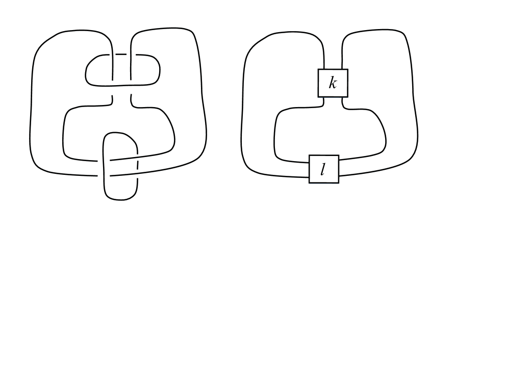
9.2. Double Twist Knots
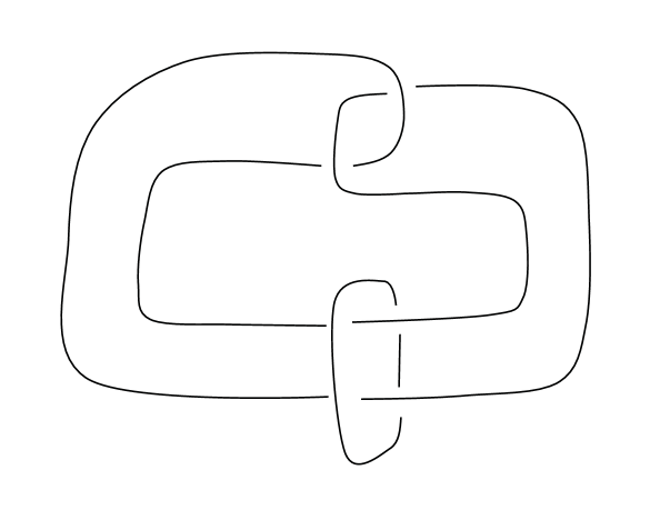
The double twist knots are the knots shown in the right hand side of Figure 4. These knots are the result of surgery and surgery on two components of the link shown in the left hand side of Figure 4 where and are the number of half twists in the boxes. The link is a knot if is even and otherwise is a two component link. Since is ambient isotopic to we may assume that . The knot complement of is hyperbolic unless or is less than two, or . The knots with or equal to two are the twist knots. These include the figure-eight knot, and the trefoil . We now restrict our attention to these hyperbolic knots.
The character varieties of these knot complements were computed in and analyzed in [14]. The component of the character variety of the double twist knot which contain irreducible representations is birationally equivalent to the curve defined by the following equations in :
| () | ||||
(The polynomials and were introduced in Definition 6.1.) These curves are smooth and irreducible in when . When the canonical component is given by . The genus can be computed from the bidegree of these polynomials. Let and and let be the projective closure of the variety determined by the equations in . When the bidegree is . The genus of is determined by studying the ramification of the map from to .
Theorem 1 ([14] Theorems 6.2 and 6.5).
Let be a hyperbolic with . If the genus of is and the genus of is where
The genus of is zero and the genus of is .
We will compute the gonality of these curves by relating the gonality to the degree of the curves. In 1883 Noether [18] proved that a non-singular plane curve of degree in has gonality equal to , where is the degree of the curve. (See [16] Theorem 2.3.1, page 73.) Certain well-behaved singularities are known to modify this relationship in an understood manner. The curves determined in [14] are smooth, but lie in ; the birational mapping to introduces singularities in the curves. We now prove a version of Noether’s theorem by understanding this mapping.
Lemma 9.1.
Let be a smooth irreducible curve in of bidegree where , then .
(If or then is isomorphic to and therefore has gonality one.)
Proof.
Consider an irreducible curve of degree . Let be the maximum multiplicity of a singular point of . The projection map from the point with multiplicity to a line has degree , so we conclude that . Ohkouchi and Sakai [19] (Theorem 3) show that if has at most two singular points (or infinitely near singular points), then . (See [15] page 194 for a discussion of infinitely near points.)
We consider the birational mapping given by
This has birational inverse given by
Let be a smooth curve of bidegree in with . It suffices to show that , , and has exactly two singular or infinitely near singular points; for then Ohkouchi and Sakai’s result implies that . Since is birational, proving the result.
If is a smooth curve of bidegree then is the vanishing set of a polynomial after projectivizing in . If the projectivization of is
When (therefore ) this reduces to . We conclude that there are points on such that . Similarly there are points corresponding to (and ). When the polynomial has a constant term, then these points do not coincide. If has no constant term, then . We will assume, by taking an isomorphic copy of , if necessary, that , so has a constant term.
Under the birational mapping, (if ). Likewise, (if ). It follows that the points above get identified, as do the points. The image in has a singularity of order and one of order . It is straightforward to see that if then a neighborhood of the point maps smoothly into . Therefore has exactly two singular points, one of degree and one of degree .
The degree of is given by the intersection number where is a hyperplane section of . Similarly, the degree of is the intersection number where is a hyperplane section of . The divisor class group of is . Let and . Then is linearly equivalent to , that is . (Two divisors are linear equivalent if their difference is a principal divisor.) The curves of bidegree correspond to the effective divisors of the class . Similarly, .
Therefore, since the degree of a divisor depends only on the linear equivalence class, . Since the degree of is the intersection number , and and it follows that the degree of is the intersection number of and , which is .
∎
We now use this to determine the gonality of the curves .
Theorem 9.2.
Let be a hyperbolic knot and let and .
-
If then .
-
If then .
Proof.
The equations defining are irreducible and determine smooth curves in by [14]. These equations have bidegree if . By Lemma 9.1 if the gonality of is . If then or and is not hyperbolic. It suffices to consider the case when . In this case, the canonical component for the character variety is isomorphic to , given by . We conclude that the gonality is one.
∎
Corollary 9.3.
For all positive integers there are infinitely many double twist knots such that
Now we compute the gonality of the canonical components of the character varieties. By Lemma 3.5 since is a degree 2 branched cover of we conclude that
We now explicitly show that the gonality equals this upper bound.
Theorem 9.4.
Let be a hyperbolic knot and let and .
-
If then .
-
If then .
Proof.
We first consider the case when . By [14], a ‘natural model’ for is given by
and is birational to the hyper elliptic curve
This has genus by [1]. If is hyperbolic then and the gonality of is two.
Now, assume that and is hyperbolic. If or is one, then one can verify directly from the defining equations that is an elliptic or hyperelliptic curve and therefore has gonality two. We will now assume that and are at least two.
Consider the following situation. Let and be smooth curves of genus and and let be a degree simple morphism and a degree morphism. (A simple morphism is one that does not factor through a nontrivial morphism.) The Castelnuovo-Severi inequality (see [3] Theorem 2.1) states that if
| () |
then factors through .
Let be a smooth projective model for and a smooth projective model for . Since there is a degree two birational map from to , by Stein factorization, there is a degree two morphism from to .
From [14], we have a degree mapping, with (for an explicitly determined ) and . Therefore, the righthand side of the inequality is
Since the right-hand side of is at most . We conclude that any dense map from to of degree at most factors through a map from to . Let be the minimal degree of a map from to . Since the gonality of is we conclude that
Since and are at least two,
By the Castelnuovo-Severi inequality, the map factors through . As the gonality of is by Lemma 9.2 we conclude that the smallest degree of a map from is .
∎
Remark 9.5.
The Brill-Noether theorem gives the bound where is the genus. For this inequality is
so the gonality is smaller than the Brill-Noether bound. For the genus of is zero and the gonality is one, meeting the Brill-Noether bound. The examples with show that for any there is a double twist knot (a twist knot, in fact) such that . That is, the discrepancy between the gonality and the Brill-Noether bound is unbounded in this family.
Remark 9.6.
Hoste and Shanahan have computed a recursive formula for the -polynomials of the twist knots [11], the knots and shown that these polynomials are irreducible. Their results show that the degree of the -polynomials grow linearly in . This shows that the linear bounds in Theorem 1.4 are sharp, since the twist knots are surgery on one component of the Whitehead link.
10. Gonality, Injectivity Radius, and Eigenvalues of the Laplacian
Since the smooth projective model of a (possibly singular) affine curve is a compact Riemann surface, it can also be viewed as a quotient of the Poincare disk by a discrete group of isometries of the Poincare disk, and as such it is natural to try to relate gonality to geometric and analytical properties associated to the hyperbolic metric; for example the injectivity radius, (i.e. half of the length of a shortest closed geodesic), or the first non-zero eigenvalue of the Laplacian, .
To that end, a famous result of Li and Yau [13] shows that for a compact Riemann surface of genus , a bound for the gonality is given by:
where is the gonality defined using regular maps. Since the (rational) gonality of a complex affine algebraic curve equals the (regular) gonality of a smooth projective completion, this bound applies to smooth projective models of character varieties. A Riemann surface of genus zero is rational and so has gonality one, and a Riemann surface of genus one is an elliptic curve and so has gonality two. For any higher genus, the above bound implies that
By Theorem 1.1 the (rational) gonality of is bounded independent of , and therefore so is the (regular) gonality, , of a smooth projective model. We conclude that is bounded above independent of for these curves. Moreover, if is sequence of rational numbers such that the genus of the character varieties grows, then since is bounded
For hyperbolic double twist knots the genera of and was determined in [14]. (See § 9.2.) The genus of is less than two only for the complements of the knots (the figure-eight) and ; both have genus 1. The only hyperbolic double twist knots such that the genus of is less than two are , , which have genus zero, and which have genus one. When , we obtain the following inequalities using Theorem 1
where and denote smooth projective models and and Both quantities as or For the once-punctured torus bundles of tunnel number one, (see § 9.1) let denote a smooth projective model. Then for
and we conclude that as .
More recently Hwang and To [12] show that the injectivity radius of a compact Riemann surface of genus is bounded above by a function of gonality (defined for regular maps),
With denoting a smooth projective model, Theorem 1.1 implies that there is a constant such that the gonality of these varieties is bounded above by and therefore there is a constant such that
It follows that the injectivity radius is bounded above for all , such that .
By Theorem 9.4 and Theorem 9.2 for all hyperbolic double twist knots other than the figure-eight, if
If then . For all once-punctured torus bundles of tunnel number one with , is a hyper elliptic curve. We conclude that for the corresponding smooth projective models the injectivity radius is bounded by
Motivated by the discussion here, we close with two questions. To state
these define an infinite family of compact Riemann surfaces
to be an expander family if the genera of
and there is a constant for which . One such
family are congruence arithmetic surfaces.
Question: (1) Does there exist an infinite family
of 1-cusped hyperbolic 3-manifolds for which (resp. )
is an expander family?
(2) Does there exist an infinite family of 1-cusped hyperbolic 3-manifolds for which (resp. ) has arbitrarily large injectivity radius?
References
- [1] Kenneth L. Baker and Kathleen L. Petersen, Character varieties of once-punctured torus bundles of tunnel number one, Internat. J. Math. 24 (2013), no. 6, 1350048 (57 pages).
- [2] S. Boyer and X. Zhang, On Culler-Shalen seminorms and Dehn filling, Ann. of Math. (2) 148 (1998), no. 3, 737–801. MR 1670053 (2000d:57028)
- [3] Youngook Choi and Seonja Kim, Gonality and Clifford index of projective curves on ruled surfaces, Proc. Amer. Math. Soc. 140 (2012), no. 2, 393–402. MR 2846309 (2012m:14064)
- [4] D. Cooper and D. D. Long, The -polynomial has ones in the corners, Bull. London Math. Soc. 29 (1997), no. 2, 231–238. MR 1426004 (98f:57026)
- [5] M. Culler and P. B. Shalen, Bounded, separating, incompressible surfaces in knot manifolds, Invent. Math. 75 (1984), no. 3, 537–545. MR 735339 (85k:57010)
- [6] Marc Culler, Lifting representations to covering groups, Adv. in Math. 59 (1986), no. 1, 64–70. MR 825087 (87g:22009)
- [7] Nathan M. Dunfield, Cyclic surgery, degrees of maps of character curves, and volume rigidity for hyperbolic manifolds, Invent. Math. 136 (1999), no. 3, 623–657. MR 1695208 (2000d:57022)
- [8] Jordan S. Ellenberg, Chris Hall, and Emmanuel Kowalski, Expander graphs, gonality, and variation of Galois representations, Duke Math. J. 161 (2012), no. 7, 1233–1275. MR 2922374
- [9] Robin Hartshorne, Algebraic geometry, Springer-Verlag, New York, 1977, Graduate Texts in Mathematics, No. 52. MR 0463157 (57 #3116)
- [10] Heisuke Hironaka, Resolution of singularities of an algebraic variety over a field of characteristic zero. I, II, Ann. of Math. (2) 79 (1964), 109–203; ibid. (2) 79 (1964), 205–326. MR 0199184 (33 #7333)
- [11] Jim Hoste and Patrick D. Shanahan, A formula for the A-polynomial of twist knots, J. Knot Theory Ramifications 13 (2004), no. 2, 193–209. MR 2047468 (2005c:57006)
- [12] Jun-Muk Hwang and Wing-Keung To, Injectivity radius and gonality of a compact Riemann surface, Amer. J. Math. 134 (2012), no. 1, 259–283. MR 2876146
- [13] Peter Li and Shing Tung Yau, A new conformal invariant and its applications to the Willmore conjecture and the first eigenvalue of compact surfaces, Invent. Math. 69 (1982), no. 2, 269–291. MR 674407 (84f:53049)
- [14] Melissa L. Macasieb, Kathleen L. Petersen, and Ronald M. van Luijk, On character varieties of two-bridge knot groups, Proc. Lond. Math. Soc. (3) 103 (2011), no. 3, 473–507. MR 2827003
- [15] Masayoshi Miyanishi, Algebraic geometry, Translations of Mathematical Monographs, vol. 136, American Mathematical Society, Providence, RI, 1994, Translated from the 1990 Japanese original by the author. MR 1284715 (95g:14001)
- [16] Makoto Namba, Families of meromorphic functions on compact Riemann surfaces, Lecture Notes in Mathematics, vol. 767, Springer, Berlin, 1979. MR 555241 (82i:32046)
- [17] Walter D. Neumann and Alan W. Reid, Rigidity of cusps in deformations of hyperbolic -orbifolds, Math. Ann. 295 (1993), no. 2, 223–237. MR 1202390 (94c:57025)
- [18] M. Noether, Zur Grundlegung der Theorie der algebraischen Raumcurven, Abhandlungen der K oniglichen Akademie der Wissenschaften, Berlin (1883).
- [19] Masahito Ohkouchi and Fumio Sakai, The gonality of singular plane curves, Tokyo J. Math. 27 (2004), no. 1, 137–147. MR 2060080 (2005d:14046)
- [20] Bjorn Poonen, Gonality of modular curves in characteristic , Math. Res. Lett. 14 (2007), no. 4, 691–701. MR 2335995 (2008k:11061)
- [21] Joan Porti, Torsion de Reidemeister pour les variétés hyperboliques, Mem. Amer. Math. Soc. 128 (1997), no. 612, x+139. MR 1396960 (98g:57034)
- [22] Igor R. Shafarevich, Basic algebraic geometry. 1, second ed., Springer-Verlag, Berlin, 1994, Varieties in projective space, Translated from the 1988 Russian edition and with notes by Miles Reid. MR 1328833 (95m:14001)
- [23] Peter B. Shalen, Representations of 3-manifold groups, Handbook of geometric topology, North-Holland, Amsterdam, 2002, pp. 955–1044. MR 1886685 (2003d:57002)
- [24] W.P. Thurston, The geometry and topology of 3-manifolds, Princeton University, Mathematics Department, 1978, available at http://msri.org/publications/books/gt3m/.
- [25] Stephan Tillmann, Boundary slopes and the logarithmic limit set, Topology 44 (2005), no. 1, 203–216. MR 2104008 (2005m:57027)
- [26] Jarosław Włodarczyk, Toroidal varieties and the weak factorization theorem, Invent. Math. 154 (2003), no. 2, 223–331. MR 2013783 (2004m:14113)