Graded Index Confined Spin Waves in an Intermediate Domain Wall
Abstract
We propose a mathematical model for describing propagating confined modes in domain walls of intermediate angle between domains. The proposed model is derived from the linearised Bloch equations of motion and after reasonable assumptions, in the scenario of a thick enough magnetic patch, are accounted. The model shows that there is a clear dependence of the local wavenumber of the confined spin wave on the local angle of the wall and excitation frequency used, which leads to the definition of a local index of refraction in the wall as a function of such angle and frequency. Therefore, the model applies to 1-D propagating modes, although it also has physical implications for 2-D scenarios where a domain wall merges with a saturated magnetic region. Micromagnetic simulations are in good agreement with the predictions of the model and also give insight on the effects of curved finite structures may have on the propagating characteristics of spin waves in domain walls.
pacs:
Valid PACS appear hereI introduction
Due to their low loss and shorter wavelength compared to electromagnetic waves in free space, spin waves are a promising candidate for information carrier in micron and sub-micron scale magnonic circuits Kruglyak et al. (2010); Karenowska et al. (2016); Hoffmann and Bader (2015). Inhomogeneities such as vortex core have been widely studied as spin waves emitters Wintz et al. (2016); Dieterle et al. (2019); Sluka et al. (2019). Once the spin wave is excited, an adequate control on its propagation is key for the developing of circuits that conducts the spin wave through channels. Local excitation of spin waves and its spatial confinement has been widely studied in terms of local ferromagnetic resonances due to inhomogeneities Davies et al. (2015a, 2017); Mushenok et al. (2017), confinement along the edges Aliev et al. (2011a); Lara et al. (2017), along domain walls and by domain wall natural fluctuations modes or so called Winter magnons Aliev et al. (2011b). Domain walls do actually act as natural channels for spin waves due to the energy well. More importantly, Winter magnons are very useful for efficiently channeling in a wide range of frequencies since they are gapless modes Winter (1961).
Graded index media for wave propagation have been widely studied specially in electromagnetics, in the field known as transformation optics Kang et al. (2008); Rinkevich et al. (2015); Pendry (2000). The development of structures ranging from nanometre size to centimetres, have proved interesting properties not shown in nature, leading to the application of novel graded-index (GRIN) lenses in an extremely wide range of frequencies, from microwaves to visible light.
In the field of magnonics, graded index magnetic media serve to similar purposes, taking advantage of the high anisotropic behaviour of spin waves Davies et al. (2015a, b). For example, tailoring the spin wave propagation in magnetic domains, allow the development of lenses for spin wavesToedt et al. (2016); Whitehead et al. (2019, 2018). Regarding uni-directional propagation in domain walls, previous studies have dealt mainly with redirection and steering the spin wave path Hamalainen et al. (2018); Albisetti et al. (2018), inducing phase changes Bayer et al. (2005); Wang and Wang (2015) or non-reciprocal paths by means of non-linear effects Garcia-Sanchez et al. (2015).
However, anisotropic magnetic media can not only modify direction, intensity, or temporal frequency of the spin wave. Spatial frequency modulation or ‘spatial chirping’ is a technique widely used in telecommunication engineering and photonics, for example, to use in fibre-Bragg gratings or other chirped mirrors as filters, where wavenumber or equivalently, wavelength (), spatially changes. Analysis of spatially chirped signals can be extended even to the processing of images where periodic features are visualised in perspective. The graded-index technique for EM waves could also have its equivalent for spin waves, and therefore, mathematical tools are required to control this feature. Using the non-uniform demagnetising field in a saturated YIG non-ellipsoidal rod, the pioneer work from Schlömann Schlömann (1964) for Backward Volume Spin waves and from Stancil Stancil and Morgenthaler (1983) for Surface Spin waves and further experimental results using spatially varying external fields Smith et al. (2008) confirmed the realization of this technique for spin waves. A change of wavelength has also been observed by using tapered saturated magnonic waveguides Demidov et al. (2011). In this article, we demonstrate a spatially dependent wavenumber (spatial dispersion) of confined modes in domain walls (and therefore, in non-saturated films), providing with an equation that allows to model their local wavenumber and propagation properties. Micromagnetic simulations on a specifically designed shape of patch, that retains in remanence a single intermediate domain wall of variable angle between two vortex cores, show good agreement with our proposed model.
II Materials and methods
To obtain insight into the dynamics, we performed a set of micromagnetic simulations using Mumax3 Vansteenkiste et al. (2014). We simulated a ‘rounded bow-tie’ shaped patch (see Fig. 3(a)) of 6000 nm length, 80 nm thickness () and 2000 nm diameter () of the circumscribed circles at the ends, with the typical material parameters of permalloy at room temperature with saturation magnetization Am-1, exchange constant Jm-1 and Gilbert damping constant for a weighted average of iron and nickel. The grid was discretized in the space into 1536 512 16 cells. The cell size along and was 3.9 nm, while the cell size along was fixed to 4 nm. The cell size along three dimensions is always kept smaller than the exchange length of permalloy (5.3 nm). The number of cells was chosen to be powers of 2 for sake of computational efficiency. We also set a ‘smooth edges’ condition with value 8. A key point in micromagnetic simulations is to achieve a stable equilibrium magnetization state. We first set a double vortex state with polarity and ‘vorticity’ numbers of (1, 1) and (1,1) and then executed the simulation with a high damping ( 1) ) to relax the magnetization until the maximum torque (‘maxtorque’ parameter in Mumax3), which describes the maximum torque/ over all cells, where is the gyromagnetic ratio of the material), reached T indicating convergence and the achievement of a magnetization equilibrium state. The typical time to achieve the equilibrium state was 100 ns. Note that this value has no direct physical meaning due to the artificial high damping. Once the ground state was obtained, damping was set back to original ( 0.008), relaxation process was repeated, the spin configuration was recorded as the ground state of the sample and then used for the simulations with the dynamic activation. For analyzing time evolution of the magnetic signal, we apply a continuous wave excitation with a magnetic field at a specific frequency in the first vortex core region only,
| (1) |
and each mode is excited with a relatively small oscillating field, mT. A sampling period of 25 ps was used, recording up to 300 simulated snap-shots in space and time, only after the steady state is reached. With these parameters, the time window of observation of the spin waves propagating in the domain wall covers up to 7.5 ns.
To numerically validate the change in wavelength predicted by the model, we run micromagnetic simulations with an excitation frequency of 1.5 GHz and 3 GHz so Winter’s magnons Winter (1961) can be efficiently launched from the core region and travel along the domain wall Garcia-Sanchez et al. (2015). Numerical results for the spatially dependent wavelength ((x)) are obtained from the time-averaged spectrograms of the channelled spin wave profiles using a Hanning window of 128 FFT points and 100 overlapping points. Since the spatial wavelength is constantly changing along the domain wall length, a fixed width of the window will introduce a trade-off between spatial frequency resolution and position accuracy in the x-direction. A wider spatial window yields less position accuracy to the wavenumber and a very narrow window cannot properly resolve the spatial frequency at large wavelengths, leading to spatial frequency leakage per frequency bin. The chosen parameters of window width and overlapping points are obtained after an optimisation process considering several different outcomes. Another solution could be using a width-variable window as described in Nisar and Tariq (2016).
III Description of the model
As a first step to a reliable model and similarly to what is done in Ref.Bayer et al. (2005), we search for an expression of a spatially dependent wavelength for a spin wave travelling in a domain wall, based on a Wentzel-Kramers-Brillouin (WKB) approximation Zilberman et al. (1995). Assuming a Neel-type domain wall along the x-direction, this implies that dynamic magnetization components at its centre can be expressed as: . As it will be shown later in this section, this description of static and dynamic magnetization is still approximately correct even for a Bloch wall of an arbitrary angle and suitable, at least, for the in-plane component of magnetization. If we assume an internal magnetic field perpendicular to the wall and only related to dipolar and exchange interactions, , where the demagnetising field is and the exchange field is . As in Ref. Bayer et al. (2005), in order to find an expression for a spatial dependent wavenumber accounting for the demagnetising field magnitude , we define a compact expression for magnetisation , assuming and neglecting the imaginary terms in order to obtain real-valued solutions, we reduce the linearised Bloch equations of motion to the following first-order, non-linear differential equation,
| (2) |
where is the excitation frequency and the gyromagnetic ratio. As a first approach to solve this differential equation, we can naively assume that variations of spin wave wavelength along the domain wall will be smooth, since no sudden changes in the demagnetizing field along the longitudinal direction are expected in a straight domain wall configuration. This implies that the first derivatives with respect to x can be neglected. Similarly to Schlömann’s work Schlömann (1964), clearing in Eq.(2) gives an approximate description for a spatially dependent wavenumber, as a function of the module of the demagnetizing field in the wall,
| (3) |
where is the wavenumber for a confined spin wave of frequency when the transversal in-plane demagnetizing field is zero, or in other words, in a 180 degrees Bloch domain wall Garcia-Sanchez et al. (2015).
Finding a general demagnetizing field expression in a non-saturated ferromagnet of a non-ellipsoidal, arbitrary shape can be a very tough task. To address this, we first provide a magnetostatic first approach for such a scenario based on how in-plane magnetization transversally changes through the wall, this is, from one domain into the other. In other words, we aim to establish a link between the Eq. (3) and the angle () between domains.
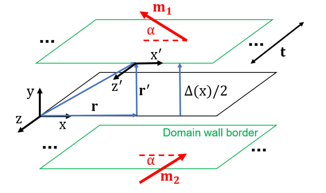
Let us assume the scenario from Fig. 1 for the domain wall of initially constant width and angle that magnetisation makes with the straight domain wall. Solving the static Landau-Lifshitz-Gilbert equation yields the Walker’s profiles across the domain wall Stancil and Prabhakar (2009). Below a critical angle , a mixed Bloch-Neel behaviour of the wall is obtained, where the Neel component is always dominant if Torok et al. (1965). A sin()-dependent coefficient is naively added to the magnetisation in-plane components transverse to the wall () to consistently model the angle dependence of a mixed wall. Following similar calculations to those shown in Ref. Hubert and Schäfer (1998), chapter 3.9 (a more detailed mathematical description of the derivation of the following equations can be found in Supplemental Material (1)), and considering that must be satisfied for every y-position across the domain wall, the three components of magnetisation in the wall region can be regarded as,
| (4) | |||
| (5) | |||
| (6) |
where
| (7) |
Following a magnetostatic approach and assuming that and , a bulk magnetic density charge () can be found,
| (8) |
The antiderivative of the latter expression effectively retrieves (Eq. (5)), which implies a ‘slow’ variation of the demagnetising field at the central region of the domain wall (), in accordance with the y-dependence of the ‘sech’ function. Notice that, if , and a cross-tie wall were formed, the term is not necessarily zero, and therefore, it should count into the expression of the bulk magnetic density charge. However, for the sake of simplicity, in this case we consider slow variations of the domain angle and domain wall’s width along the domain wall’s length ( and ) and no formation of a cross-tie profile. This implies that . Also, a thick enough patch is considered, so at the central region of the patch, far enough from the surface pinning effects, variations of magnetization across the thickness can also be neglected () even considering the formation of a cross-tie wall Metlov (2001). Under the above mentioned assumptions and due to the conservation of the transverse component in the domain wall border (following on the schematic from Fig. 1), surface magnetic charges can also be considered negligible (). Choosing the right integration volume under reasonable assumptions, for example a rectangular prism of chosen dimensions equivalent to the domain wall width () in the x- and y-directions and to the thickness () in the z-direction, an expression of the demagnetising field can be found. This expression, derived from the magnetostatic potential obtained in turn from the defined magnetic density charge, Eq. (8) (see Supplemental Material (2)), is,
| (9) |
where is the thickness of the magnetic patch and the ‘constant’ domain wall width. A more detailed derivation of Eq.(9) is shown in the Supplemental Material (2). Note that Eq. (9) is only valid for values of in the wall region (). Also, Eq. (9) yields a numerical indeterminate at the centre of the wall although this is not a physically realisable solution. At the midwidth (taking the limit ) of the domain wall, where the confinement of the mode is strongest (in accordance with the maximum of the ‘sech’ function), and assuming in a thick enough sample, Eq. (9) finally leads to
| (10) |
This equation allows to express the demagnetizing field perpendicular to the wall, in terms of the arbitrary angle α of magnetization between the magnetic domains and the wall. Moreover, it is also consistent with the assumption of a dominant Neel component in the domain wall profile.
After obtaining the compact expression from Eq.(10), it is worth noting that at an angle of there is, by definition, no domain wall since magnetisation is ‘continuous’. The wall width is by definition ‘zero’ and the model no longer applies. The competition between dipolar and exchange energies means that this angle α will also determine the width of the domain wall. In other words, finding an expression for the demagnetising field as a function of the domain angles and the domain wall width is a self-consistent problem. In order to find. In order to find a more complete and exact expression for , an additional demagnetising field should be derived from the respective magnetic potential, again derived from the magnetic density charges defined by . These considerations along with a variable domain wall width add more complexity to the model. However, as described before, the following reasonable assumptions can be made for sake of simplicity in our approximate model: (1) Since the maximum intensity of the confined mode will be at the centre of the domain wall (), the quotient is very small regardless of the domain wall width while , or equivalently, for . Under this condition is where the proposed model is intended to be used. Due to the equivalence between and ‘y’ when , replacing the first term by just ‘y’ in the equation avoids the dependence on the wall width ()); and (2), the main assumption for these results is that the demagnetising field is orientated, almost fully in-plane and perpendicular to the domain wall. This assumption is not far from reality, since it has been proved that, in intermediate domain walls (between 180°-Bloch and Neel wall), the Neel component is dominant. This behaviour is observed in arbitrary α-Bloch walls where °. In fact, above a critical angle, the out-of-plane component of magnetisation vanishes, and the wall becomes essentially a Neel wall Olson et al. (1967). Not only that, argument is even more convincing for thicker samples, since the critical angle reduces when increasing thickness almost reaching zero when Torok et al. (1965). Eq.(10) is consistent with these results, since it also reduces in magnitude as reduces.
After all these considerations, we need to stress, once again, that finding an exact solution for a local demagnetising field is very often, a very complicated task for non-ellipsoidal shapes, even in saturation or quasi-saturation Osborn (1945); Berkov and Gorn (2005). When not found numerically through micromagnetic simulations, approximate analytical approaches are usually taken under reasonable assumptions DeJong and Livesey (2015). For all this and realizing that Eq. (10) is a physically consistent model for the defined scenario, we consider it from now on, as a valid first approximation for the transverse demagnetising field along a domain wall of variable domain angle. Therefore, this expression can be combined with Eq. (3) to give a new one where the dependence is now with the variable angle between magnetic domains,
| (11) |
This equation relies on an initial k ( x) which is found to be the wavenumber of a Winter’s magnon for a frequency through a 180° domain wall (i.e., when ). Regarding this, through the dispersion relation of Winter’s magnons, a spatial index of refraction can be defined as ,
| (12) |
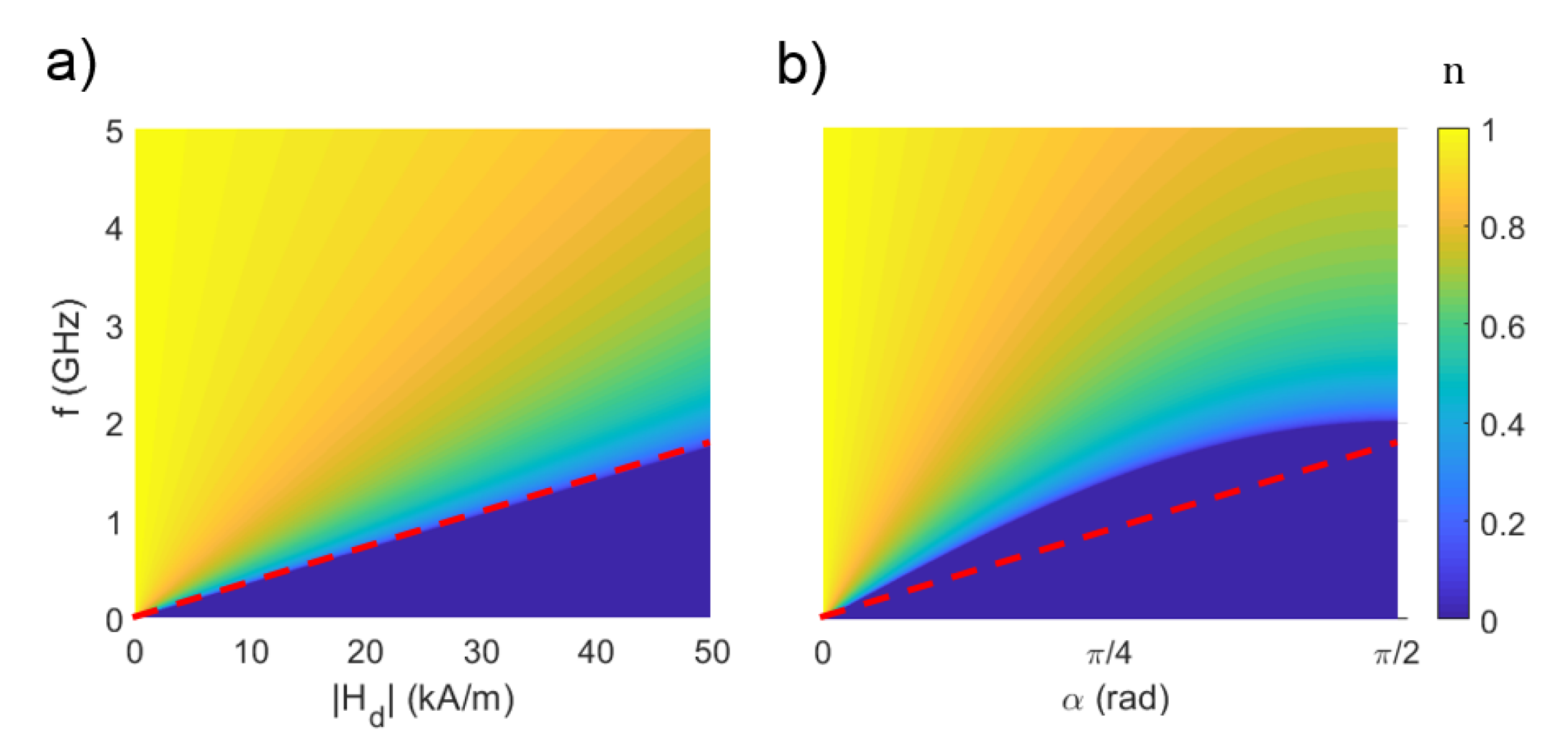
where and is the frequency of a continuous wave excitation. This equation predicts the change in wavenumber (or wavelength) from a given along the domain wall. In other words, a different initial will give different values of local wavenumbers, but always varying in accordance to this model. Therefore, this applies as well to the index of refraction if we assume an index of unity for an arbitrary initial . Fig. 2(a) shows a contour plot of the real values of Eq. (12) as a function of the magnitude of and . It clearly shows, for the right combination for excitation frequency and a generic demagnetising field magnitude, the different values for the real part of the index of refraction (dark blue area shows an entirely imaginary index). Most importantly, it shows how at lower frequencies, the change in wavenumber is more sensitive to the transversal demagnetising field than at higher frequencies. Fig. 2(b) shows the same behaviour even when Eq. (10) is introduced into Eq. (12), which reflects now the dependence on the angle .
It can be inferred from Eq.(12) that, in absence of a biasing field, there is an upper limit for the frequency at which an index of refraction of zero can be obtained. This maximum is reached when the demagnetising field is maximal. In principle, in terms of the magnetic moments’ orientation, this is when . However, notice that, in this situation, the definition of domain wall is meaningless. The scenario would imply the vanishing of the domain wall into a saturated region in the y-direction (i.e., a magnetic domain). In that region, Eq.(12) can be modified by replacing the formerly dominant demagnetising field from the (also former) domain wall by an expression of an effective or internal magnetic field . Interestingly, Eq.(12) implies that an index of refraction of zero would be obtained at , which is actually the ferromagnetic resonance main mode (i.e., all precessions in phase) of a saturated film for a given internal field . This result agrees with the wave perspective of a uniform FMR precession, which lays a wavenumber of (infinite wavelength and ). Additional simulations (see Supplemental Material (3)), show that at this combination of frequency and effective field, the FMR main mode is not necessarily excited in the saturated region but instead, a spin wave mode with at least (but not necessarily ) can be excited (i.e., a Backward Volume Spin Wave mode). This result still agrees with the perspective of a ‘confined mode’ in the x-direction, since the model becomes a loose approximation to a scenario where domains or saturated regions are present. In other words, it does not account for modes that may show non-zero wavenumber in a different direction of propagation, such as the y-direction, orthogonal to the original domain wall, although it effectively retrieves the expected zero wavenumber in the x-direction. More interestingly, the model predicts the existence of, conceptually speaking, evanescent spin waves below that ‘pseudo-FMR’ frequency condition.
IV Numerical validation
A mathematical model is only as good as the assumptions. In order to validate our model for the real values obtained from Eq.(12), micromagnetic simulations on the magnetic structure shown in Fig. 3 are performed and recorded for comparison with the analytical model. Since it is inevitable to start from an angle of approximately at the source (the vortex core), the shape of this structure has been chosen so because it allows to cover the widest range of values of and therefore of n, see Fig.4. Therefore, for the shape of this patch, the demagnetizing field transversal to the wall is not constant along its length: The angle at both sides of the wall changes from at the core region to 0 at the centre of the shape and to back again.
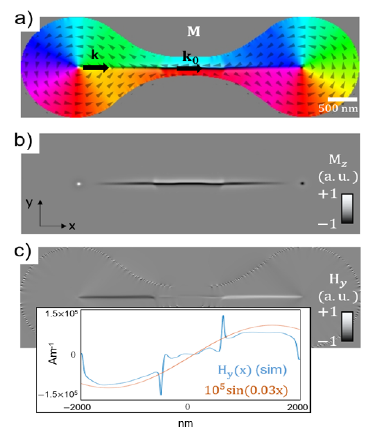
Notice that, as reference, an index of refraction of unity midway between the vortex cores, in a 180° Bloch wall, is considered. The reference wavenumber is that of a Winter’s magnon along a 180° Bloch wall. For a spin wave propagating from one of the core regions, reduction in (or equivalently, reduction in the transverse demagnetizing field, see Fig. 3(c)) implies an increase in the local wavenumber. From numerical results on this particular shape, small and smooth variations of the angle are considered far from the core regions, so the assumption and is still hold and therefore: . Close to the core regions, the domain wall angle is large enough to assume the domain wall Neel component to be dominant Olson et al. (1967) and therefore, is also satisfied at the centre of the domain wall. In other words, the assumptions held in the previous section are still valid as well as the derived model for the demagnetising field transverse to the wall.
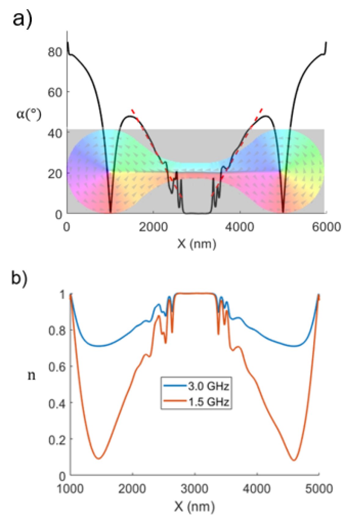
Fig. 4(a) shows the spatial position profile of α parallel to the domain wall at 50 nm from the centre of the wall, calculated as , where the components of magnetisation are extracted from numerical simulations and magnetisation is assumed in-plane. The ripples close to the central region come from the numerically obtained equilibrium state of magnetic moments. More specifically, from those in the region where the curved contour is closer to the straight domain wall, which makes magnetization to not smoothly follow the contour neither the domain wall in a straight line but rather, in an apparent ‘zig-zagging’ path as a middle-ground solution. This alters the calculation of the angle (), introducing the rippling. Ideally, this should not be happening, and magnetisation should be laying completely in-plane and smoothly following the shape contour even close to the domain wall. Still, the shape of the structure allows to approximate the dependence of angle α with x by a fitting linear dependence , see red dotted line in Fig. 4(a), making it closer to the ideal case. Including this linear fitting into the proposed model for the demagnetising field (Eq. 10) shows also good qualitative agreement with the values obtained from simulations (see inset in Fig. 3(c)).
Quantitatively, result from simulation fits better to a sinusoidal function with a maximum value of Am-1. While in the same order of magnitude, this value is about three times the maximum of the model from Eq. (10) for , Am-1, (for a saturation magnetisation of Am-1). This can be explained by the neglection of other components of the magnetostatic potential in the model (which leads to a ‘weaker’ demagnetising field than in reality, due to fewer contributions), that should be accounted for a more accurate description.
Fig. 4(b) shows the analytical index of refraction from Eq. (12) with the obtained values of α as inputs for the excitation frequencies of 1.5 GHz and 3 GHz. This agrees with analytical results from Fig. 2(b), at 3 GHz excitation frequency, which show that the wavevector can be reduced as much as approximately 0.7 times the reference wavevector (i.e., ) when the spin wave approaches the core regions (at 900 nm from the vortex core) and is approximately radians (i.e., 37°, see Fig. 4(a)).
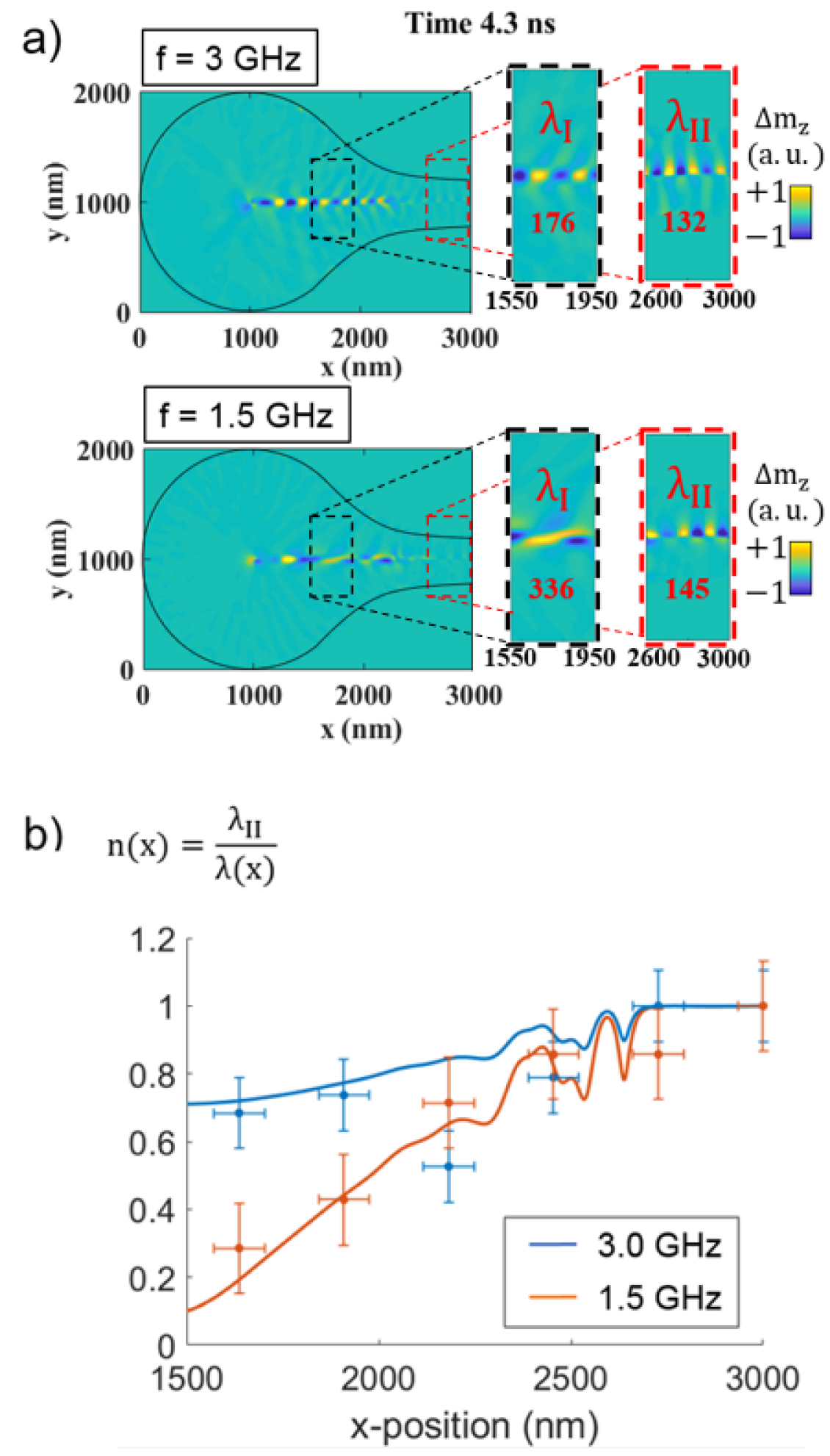
Fig. 5(a) shows the wave profile of the propagating mode and the respective wavelengths found in the respective regions I () and II () (insets). A significant attenuation of the spin wave is observed in region II (the colour intensity in the insets is manually adjusted for ease of comparison), we believe this is originated by the ‘zig-zagging’ path of magnetisation in the domains which induces a pronounced gradient in the local demagnetising field halfway between the two regions (see blue curve in the inset of Fig. 3(c)), modifying in turn the spatially local ferromagnetic resonance in the wall and thus presenting low transmission between regions in the wall Wang et al. (2013); Chang et al. (2018), as a 1-D analogy of the 2-D scenario explored in Ref.Chang et al. (2018). Fig. 5(b) shows the index of refraction profiles for 1.5 GHz and 3 GHz (solid lines) obtained from Eq.(12), with the range of angles found from simulations as input, and numerical results (dots) for the spatial frequency in the x-direction, normalised to the value at 3000 nm (or in other words, the simulated spatial index of refraction). Numerical results confirm what the equation predicted: The change in wavenumber is more pronounced, and more sensitive to the transverse demagnetising field (or equivalently, to the domain angle ) when the frequency is smaller. Therefore, the covered graded-index profile is wider at lower frequencies. Also, as expected from the model, the values of the obtained index of refraction from simulations agrees with the predicted values from Eq. (12) with the specified angle ° at the corresponding position (x = 1900 nm) in the shape ( at 3 GHz and at 1.5 GHz). An apparent physical anomaly for an excitation frequency of 3 GHz is observed from simulations (blue dots in Fig. 5(b)) halfway between the regions I and II, i.e. around x = 2200 nm. The x-positions near that value actually correspond to the region where the ‘zig-zagging’ of magnetisation is more marked, making the simulated value not comparable to the value from the model, that assumes a smooth variation of the demagnetising field. This explains the considerable mismatch at around x = 2200 nm in Fig. 5(b), and shows that the effects of curved edges on propagation in a straight domain wall might be difficult to avoid in certain localised areas in a finite structure and more significant for higher excitation frequencies.
In conclusion, Eq. (11) or its generic form Eq. (3) is proposed as a valid model for finding the local wavenumber (and Eq. (12) for the local index of refraction) of a spin wave along domain walls under the influence of different demagnetising fields or shape contour effects. The model helps to predict how these effects modify the wavelength of a confined mode in a domain wall.
V Summary
The main result of this work is the proposed mathematical model for an effective spatial frequency dependence of confined spin waves in an ‘intermediate angle’ domain walls as a function of that angle. The equation of the model is derived from the fundamental Bloch equations of motion, an approximated (under reasonable assumptions, similar to those in Ref. DeJong and Livesey (2015) expression of the demagnetising field transversal to the wall, that is applied to a variety of magnonic scenarios. The model can be applied to straight domain walls of variable domain angles, which can be useful as a first approximation to the study of more complex scenarios such as spin waves in confined structures of arbitrary shapes showing magnetic domains. Reciprocally, the connection between the shape of the magnetic ‘patch’ and the shape-induced demagnetising field transverse to the wall, allows us to design its shape for a particularly desired channelled spin wave profile.
The model also leads to conditions that have physical meaning such as the FMR main mode frequency or Backward Volume Spin Waves, and therefore further extending the applicability of the model to not localised modes in domain walls. In summary, an equation for a spatial-dependent wavenumber for spin waves is proposed, performing as a good model for their propagating behaviour in domain walls. This result may help in the development of more complex models for spin wave propagation in non-saturated nanostructures, channelled along domain walls or propagating into magnetic domains.
VI Acknowledgements
This work was supported by EPSRC and the CDT in Metamaterials, University of Exeter. All data created during this research are openly available from the University of Exeter’s institutional repository at https://ore.exeter.ac.uk/repository/
References
- Kruglyak et al. (2010) V. V. Kruglyak, S. O. Demokritov, and D. Grundler, Journal of Physics D: Applied Physics 43, 264001 (2010).
- Karenowska et al. (2016) A. D. Karenowska, A. V. Chumak, A. A. Serga, and B. Hillebrands, “Magnon spintronics,” in Handbook of Spintronics, edited by Y. Xu, D. D. Awschalom, and J. Nitta (Springer Netherlands, Dordrecht, 2016) pp. 1505–1549.
- Hoffmann and Bader (2015) A. Hoffmann and S. D. Bader, Phys. Rev. Applied 4, 047001 (2015).
- Wintz et al. (2016) S. Wintz, V. Tiberkevich, M. Weigand, J. Raabe, J. Lindner, A. Erbe, A. Slavin, and J. Fassbender, Nature Nanotechnology, 11 (2016).
- Dieterle et al. (2019) G. Dieterle, J. Förster, H. Stoll, A. S. Semisalova, S. Finizio, A. Gangwar, M. Weigand, M. Noske, M. Fähnle, I. Bykova, J. Gräfe, D. A. Bozhko, H. Y. Musiienko-Shmarova, V. Tiberkevich, A. N. Slavin, C. H. Back, J. Raabe, G. Schütz, and S. Wintz, Phys. Rev. Lett. 122, 117202 (2019).
- Sluka et al. (2019) V. Sluka, T. Schneider, R. Gallardo, A. Kakay, M. Weigand, T. Warnatz, R. Mattheis, A. Roldán-Molina, P. Landeros, V. Tiberkevich, A. Slavin, A. Erbe, A. Deac, J. Lindner, J. Raabe, J. Fassbender, and S. Wintz, Nature Nanotechnology 14 (2019), 10.1038/s41565-019-0383-4.
- Davies et al. (2015a) C. Davies, A. Francis, A. Sadovnikov, S. Chertopalov, M. Bryan, S. Grishin, D. Allwood, Y. Sharaevskii, S. Nikitov, and V. Kruglyak, Physical Review B - Condensed Matter and Materials Physics, 92 (2015a).
- Davies et al. (2017) C. S. Davies, V. D. Poimanov, and V. V. Kruglyak, Phys. Rev. B 96, 094430 (2017).
- Mushenok et al. (2017) F. B. Mushenok, R. Dost, C. S. Davies, D. A. Allwood, B. J. Inkson, G. Hrkac, and V. V. Kruglyak, Applied Physics Letters 111, 042404 (2017), https://doi.org/10.1063/1.4995991 .
- Aliev et al. (2011a) F. G. Aliev, A. A. Awad, D. Dieleman, A. Lara, V. Metlushko, and K. Y. Guslienko, Phys. Rev. B 84, 144406 (2011a).
- Lara et al. (2017) A. J. Lara, J. R. Moreno, K. Y. Guslienko, and F. G. Aliev, in Scientific Reports (2017).
- Aliev et al. (2011b) F. G. Aliev, A. A. Awad, D. Dieleman, A. Lara, V. Metlushko, and K. Y. Guslienko, Phys. Rev. B 84, 144406 (2011b).
- Winter (1961) J. M. Winter, Phys. Rev. 124, 452 (1961).
- Kang et al. (2008) L. Kang, Q. Zhao, H. Zhao, and J. Zhou, Opt. Express 16, 8825 (2008).
- Rinkevich et al. (2015) A. Rinkevich, S. Demokritov, M. Samoilovich, and O. Nemytova, Photonics and Nanostructures - Fundamentals and Applications 15 (2015), 10.1016/j.photonics.2015.03.004.
- Pendry (2000) J. B. Pendry, Phys. Rev. Lett. 85, 3966 (2000).
- Davies et al. (2015b) C. S. Davies, A. Francis, A. V. Sadovnikov, S. V. Chertopalov, M. T. Bryan, S. V. Grishin, D. A. Allwood, Y. P. Sharaevskii, S. A. Nikitov, and V. V. Kruglyak, Phys. Rev. B 92, 020408 (2015b).
- Toedt et al. (2016) J.-N. Toedt, M. Mundkowski, D. Heitmann, S. Mendach, and W. Hansen, Scientific Reports 6 (2016).
- Whitehead et al. (2019) N. J. Whitehead, S. A. R. Horsley, T. G. Philbin, and V. V. Kruglyak, Phys. Rev. B 100, 094404 (2019).
- Whitehead et al. (2018) N. J. Whitehead, S. A. R. Horsley, T. G. Philbin, and V. V. Kruglyak, Applied Physics Letters 113, 212404 (2018), https://doi.org/10.1063/1.5049470 .
- Hamalainen et al. (2018) S. Hamalainen, M. Madami, H. Qin, G. Gubbiotti, and S. Dijken, Nature Communications 9 (2018), 10.1038/s41467-018-07372-x.
- Albisetti et al. (2018) E. Albisetti, D. Petti, G. Sala, R. Silvani, S. Tacchi, S. Finizio, S. Wintz, A. Calò, X. Zheng, J. Raabe, E. Riedo, and R. Bertacco, Communications Physics 1 (2018), 10.1038/s42005-018-0056-x.
- Bayer et al. (2005) C. Bayer, H. Schultheiss, B. Hillebrands, and R. Stamps, Institute of Electrical and Electronics Engineers Transactions on Magnetics 41, 3094 (2005).
- Wang and Wang (2015) X. S. Wang and X. R. Wang, “Domain walls as spin wave waveguides,” (2015), arXiv:1512.05965 [cond-mat.mes-hall] .
- Garcia-Sanchez et al. (2015) F. Garcia-Sanchez, P. Borys, R. Soucaille, J.-P. Adam, R. L. Stamps, and J.-V. Kim, Phys. Rev. Lett. 114, 247206 (2015).
- Schlömann (1964) E. Schlömann, Journal of Applied Physics 35, 159 (1964), https://doi.org/10.1063/1.1713058 .
- Stancil and Morgenthaler (1983) D. D. Stancil and F. R. Morgenthaler, Journal of Applied Physics 54, 1613 (1983), https://doi.org/10.1063/1.332146 .
- Smith et al. (2008) K. R. Smith, M. J. Kabatek, P. Krivosik, and M. Wu, Journal of Applied Physics 104, 043911 (2008), https://doi.org/10.1063/1.2963688 .
- Demidov et al. (2011) V. E. Demidov, M. P. Kostylev, K. Rott, J. Münchenberger, G. Reiss, and S. O. Demokritov, Applied Physics Letters 99, 082507 (2011), https://doi.org/10.1063/1.3631756 .
- Vansteenkiste et al. (2014) A. Vansteenkiste, J. Leliaert, M. Dvornik, M. Helsen, F. Garcia-Sanchez, and B. Van Waeyenberge, AIP Advances 4, 107133 (2014), https://doi.org/10.1063/1.4899186 .
- Nisar and Tariq (2016) K. O. U. Nisar, S. and M. Tariq, Computational intelligence and neuroscience 2016, 6172453 (2016).
- Zilberman et al. (1995) P. E. Zilberman, A. G. Temiryazev, and M. P. Tikhomirova, Journal of Experimental and Theoretical Physics 81 (1995).
- Stancil and Prabhakar (2009) D. D. Stancil and A. Prabhakar, in Spin Waves: Theory and Applications (Springer, Boston, MA, 2009).
- Torok et al. (1965) E. J. Torok, A. L. Olson, and H. N. Oredson, Journal of Applied Physics 36, 1394 (1965).
- Hubert and Schäfer (1998) A. Hubert and R. Schäfer, in Magnetic Domains: The Analysis of Magnetic Microstructures (Springer-Verlag Berlin Heidelberg, 1998).
- Metlov (2001) K. L. Metlov, Applied Physics Letters 79, 2609 (2001), https://doi.org/10.1063/1.1409946 .
- Olson et al. (1967) A. L. Olson, H. N. Oredson, E. J. Torok, and R. A. Spurrier, Journal of Applied Physics 38, 1349 (1967).
- Osborn (1945) J. A. Osborn, Phys. Rev. 67, 351 (1945).
- Berkov and Gorn (2005) D. Berkov and N. Gorn, Phys. Rev. B 71, 052403 (2005).
- DeJong and Livesey (2015) M. D. DeJong and K. L. Livesey, Phys. Rev. B 92, 214420 (2015).
- Wang et al. (2013) X.-G. Wang, G.-H. Guo, G.-F. Zhang, Y.-Z. Nie, and Q.-L. Xia, Journal of Applied Physics 113, 213904 (2013), https://doi.org/10.1063/1.4808298 .
- Chang et al. (2018) L.-J. Chang, Y.-F. Liu, M.-Y. Kao, L.-Z. Tsai, J.-Z. Liang, and S.-F. Lee, Scientific Reports 8 (2018), 10.1038/s41598-018-22272-2.