Gradient Estimation with Discrete Stein Operators
Abstract
Gradient estimation—approximating the gradient of an expectation with respect to the parameters of a distribution—is central to the solution of many machine learning problems. However, when the distribution is discrete, most common gradient estimators suffer from excessive variance. To improve the quality of gradient estimation, we introduce a variance reduction technique based on Stein operators for discrete distributions. We then use this technique to build flexible control variates for the REINFORCE leave-one-out estimator. Our control variates can be adapted online to minimize variance and do not require extra evaluations of the target function. In benchmark generative modeling tasks such as training binary variational autoencoders, our gradient estimator achieves substantially lower variance than state-of-the-art estimators with the same number of function evaluations.
1 Introduction
Modern machine learning relies heavily on gradient methods to optimize the parameters of a learning system. However, exact gradient computation is often difficult. For example, in variational inference for training latent variable models [43, 29], policy gradient algorithms in reinforcement learning [65], and combinatorial optimization [40], the exact gradient features an intractable sum or integral introduced by an expectation under an evolving probability distribution. To make progress, one resorts to estimating the gradient by drawing samples from that distribution [50, 39].
The two main classes of gradient estimators used in machine learning are the pathwise or reparameterization gradient estimators [29, 47, 58] and the REINFORCE or score function estimators [65, 18]. The pathwise estimators have shown great success in training variational autoencoders [29] but are only applicable to continuous probability distributions. The REINFORCE estimators are more general-purpose and easily accommodate discrete distributions but often suffer from excessively high variance.
To improve the quality of REINFORCE estimators, we develop a new variance reduction technique for discrete expectations. Our method is based upon Stein operators [see, e.g., 55, 1], computable functionals that generate mean-zero functions under a target distribution and provide a natural way of designing control variates (CVs) for stochastic estimation.
We first provide a general recipe for constructing practical Stein operators for discrete distributions (Table 1), generalizing the prior literature [9, 25, 16, 8, 46, 67, 6]. We then develop a gradient estimation framework—RODEO—that augments REINFORCE estimators with mean-zero CVs generated from Stein operators. Finally, inspired by Double CV [60], we extend our method to develop CVs for REINFORCE leave-one-out estimators [49, 30] to further reduce the variance.
The benefits of using Stein operators to construct discrete CVs are twofold. First, the operator structure permits us to learn CVs with a flexible functional form such as those parameterized by neural networks. Second, since our operators are derived from Markov chains on the discrete support, they naturally incorporate information from neighboring states of the process for variance reduction.
We evaluate RODEO on 15 benchmark tasks, including training binary variational autoencoders (VAEs) with one or more stochastic layers. In most cases and with the same number of function evaluations, RODEO delivers lower variance and better training objectives than the state-of-the-art gradient estimators DisARM [14, 69], ARMS [13], Double CV [60], and RELAX [20].
2 Background
We consider the problem of maximizing the objective function with respect to the parameters of a discrete distribution . Throughout the paper we assume is a differentiable function of real-valued inputs but is only evaluated at a discrete subset due to the discreteness of .111This assumption holds for many discrete probabilistic models [21] including the binary VAEs of Section 6. Exact computation of the expectation is typically intractable due to the complex nature of and . The standard workaround is to rewrite the gradient as and employ the Monte Carlo gradient estimator known as the score function or REINFORCE estimator [18, 65]:
| (REINFORCE) |
Here, is a constant called the “baseline” introduced to reduce the variance of the estimator by reducing the scaling effect of . Since , the REINFORCE estimator is unbiased for any choice of , and the term is known as a control variate (CV) [42, Ch. 8]. The optimal baseline can be estimated using additional function evaluations [64, 7, 45]. A simpler approach is to use moving averages of from historical evaluations or to train function approximators to mimic those values [37]. When , a powerful variant of REINFORCE is obtained by replacing with the leave-one-out average of function values:
| (RLOO) |
This approach is often called the REINFORCE leave-one-out (RLOO) estimator [49, 30, 48] and was recently observed to have very strong performance in training discrete latent variable models [48, 14].
All the above methods construct a baseline that is independent of the point under consideration, but there are other ways to preserve the unbiasedness of the estimator. We are free to use a sample-dependent baseline as long as the expectation is easily computed or has a low-variance unbiased estimate. In this case, we can correct for any bias introduced by by adding in this expectation: For example, can be a lower bound or a Taylor expansion of [43, 22]. Taking this a step further, the Double CV estimator [60] proposed to treat as the effective objective function and apply the leave-one-out idea:
The resulting estimator adds two CVs to RLOO: the global CV and the local CV . Intuitively, is aimed at reducing the variance of the LOO average. This is motivated by the fact that replacing with in RLOO leads to lower variance [60, Prop 1]. To obtain a tractable correction term , Titsias and Shi [60] adopt a linear design of : for and a coefficient .
Although the Double CV framework points to a promising new direction for developing better REINFORCE estimators, one only obtains significant reduction in variance when is strongly correlated with . This may fail to hold for the above linear and a highly nonlinear , especially in applications like training deep generative models.
In the following two sections, we will introduce a method that allows us to use very flexible CVs while still maintaining a tractable correction term. Our method enables online adaptation of CVs to minimize gradient variance (similar to RELAX [20]) but does not assume has a continuous reparameterization. We then apply it to generalize the linear CVs in Double CV to very flexible ones such as neural networks. Moreover, we provide an effective CV design based on surrogate functions that requires no additional evaluation of compared to RLOO.
3 Control Variates from Discrete Stein Operators
At the heart of our new estimator is a technique for generating flexible discrete CVs, that is for generating a rich class of functions that have known expectations under a given discrete distribution . One way to achieve this is to identify any discrete-time Markov chain with stationary distribution . Then, the transition matrix , defined via , satisfies and hence
| (1) |
for any integrable function . We overload our notation so that, for any suitable matrix , . In other words, for any integrable , the function is a valid CV as it has known mean under . Moreover, the linear operator is an example of a Stein operator [55, 1] in the sense that it generates mean-zero functions under . In fact, both Stein et al. [56] and Dellaportas and Kontoyiannis [12] developed CVs of the form based on reversible discrete-time Markov chains and linear input functions .
More generally, Barbour [3] and Henderson [23] observed that if we identify a continuous-time Markov chain with as its stationary distribution, then the generator , defined via
| (2) |
satisfies and hence for all integrable . Therefore, is also a Stein operator suitable for generating CVs. Moreover, since any discrete-time chain with transition matrix can be embedded into a continuous-time chain with transition rate matrix , this continuous-time construction is strictly more general [57, Ch. 4].
3.1 Discrete Stein operators
We next present several examples of broadly applicable discrete Stein operators (summarized in Table 1) that can serve as practical defaults.
Gibbs Stein operator The transition kernel of the random-scan Gibbs sampler with stationary distribution [see, e.g., 17] is
| (3) |
where is the indicator function, denotes all elements of except . The associated Stein operator is with
| (4) |
In the binary variable setting, 4 recovers the operator Bresler and Nagaraj [8], Reinert and Ross [46] used to bound distances between the stationary distributions of Glauber dynamics Markov chains.
Zanella Stein operator Zanella [70] studied continuous-time Markov chains with generator
| (5) |
where denotes the transition neighborhood of and is a continuous positive function satisfying . Conveniently, the neighborhood structure can be arbitrarily sparse. Moreover, the constraint ensures that the chain satisfies detailed balance (i.e., ) and hence that . Hodgkinson et al. [24] call the associated operator the Zanella Stein operator:
| (6) |
Important special cases include the minimum probability flow [53] (MPF) Stein operator () discussed in Barp et al. [6] and the Barker [4] Stein operator ().
Birth-death Stein operator Let represent the standard basis vectors on . For any finite-cardinality space, we may index the elements of , let return the index of the element that represents, and define the increment and decrement operators
Then the product birth-death process [28] on with birth rates , death rates , and generator
has as a stationary distribution, as . This construction yields the birth-death Stein operator
| (7) |
An analogous operator is available for countably infinite [24], and Brown and Xia [9], Holmes [25], Eichelsbacher and Reinert [16] used related operators to characterize convergence to discrete target distributions. Moreover, by substituting in 7, we recover the difference Stein operator proposed by Yang et al. [67] without reference to birth-death processes:
| (8) |
Choosing a Stein operator Despite being better-known, the difference and MPF operators often suffer from large variance and numerical instability due to their use of unbounded probability ratios . As a result, we recommend the numerically stable Gibbs operator when each component of is binary or takes on a small number of values. When takes on a large number of values (), the Gibbs operator suffers from linear scaling with . In this case, we recommend the Barker operator where a sparse neighborhood structure can be specified, such as . The Barker operator is numerically stable as its .
4 Gradient Estimation with Discrete Stein Operators
Recall that REINFORCE estimates the gradient Due to the existence of as a weighting function, we apply a discrete Stein operator to a vector-valued function per dimension to construct the following estimator with a mean-zero CV:
| (9) |
Ideally, we want to choose the such that strongly correlates with to reduce its variance. The optimal that yields zero variance is given by the solution of Poisson equation
| (10) |
We could learn a separate per dimension to approximate the solution of 10. However, this poses a difficult optimization problem that requires simultaneously solving Poisson equations. Instead, we will incorporate knowledge about the structure of the solution to simplify the optimization.
To determine a candidate functional form for , we draw inspiration from an “optimal” Markov chain in which the current state is ignored entirely and the new state is generated independently from . In this case, becomes , and the optimal solution is . Inspired by this, we consider of the form
| (11) |
where we now only need to learn a scalar-valued function . Notably, when exactly equals and for any discrete time Markov chain kernel , our CV adjustment amounts to Rao-Blackwellization [42, Sec. 8.7], as we end up replacing with its conditional expectation . This yields a guaranteed variance reduction.
Surrogate function design Based on the above reasoning, we can view as a surrogate for . We avoid directly setting because our Stein operators evaluate at all neighbors of the sample points, and can be very expensive to evaluate [see, e.g., 51]. To avoid this problem, we first observe that 11 can be made sample-specific, i.e., we can use a different for each sample point :
| (12) |
We then consider the following choices of that are informed about while being cheap to evaluate:
| (13) |
Here belongs to a flexible parametric family of functions such as neural networks and is chosen to have significantly lower cost than . will take on the values of and its neighbors in the Markov chain. We omit in the sum 13 to ensure that the function is independent of and hence that . Moreover, this surrogate function design introduces no additional evaluations of beyond those required for the usual RLOO estimator. Also, as observed by Titsias and Shi [60], for many applications, including VAE training, where has parameters learned through gradient-based optimization, can be obtained “for free” from the same backpropagation used to compute (see Algorithm 1).
RODEO We can further improve the estimator by leveraging discrete Stein operators and the above surrogate function design to construct both the global and local CVs in the Double CV framework [60] (see Section 2). We call our final estimator RODEO for RLOO with Discrete StEin Operators:
| (RODEO) |
where and are scalar-valued functions. Here, is a scalar-valued CV introduced to reduce the variance of the leave-one-out baseline , while acts as a global CV to further reduce the variance of the gradient estimate. We adopt the aforementioned design of 13 and 11 for the two CVs. In Appendix B, we show that the RODEO estimator is unbiased for when each is defined as in 13 and
| (14) |
Optimization with RODEO In practice, we let the functions and share a neural network architecture with two output units. Since the estimator is unbiased, we can optimize the parameters of the network in an online fashion to minimize the variance of the estimator (similar to [20]). Specifically, if we denote the RODEO gradient estimate by , then In Algorithm 1, we use an unbiased estimate of this hyperparameter gradient, , to update after each optimization step of .
5 Related Work
As we have seen in Section 2, there is a long history of designing CVs for REINFORCE estimators using “baselines” [64, 7, 45, 37]. Recent progress is mostly driven by leave-one-out [49, 38, 30, 48] and sample-dependent baselines [43, 22, 60, 62, 20]. REBAR [62] constructs the baseline through continuous relaxation of the discrete distribution [26, 35] and applies reparameterization gradients to the correction term. As a result REBAR uses three evaluations of for each instead of the usual single evaluation (see Appendix A for a detailed explanation). The RELAX [20] estimator generalizes REBAR by noticing that their continuous relaxation can be replaced with a free-form CV. However, in order to get strong performance, RELAX still includes the continuous relaxation in their CV and only adds a small deviation to it. Therefore, RELAX also uses three evaluations of for each and is usually considered more expensive than other estimators.
An attractive property of the RODEO estimator is that it incorporates information from neighboring states thanks to the Stein operator while avoiding additional costly evaluations thanks to the learned surrogate functions . Estimators based on analytic local expectation [59, 61] and GO gradients [11] also use neighborhood information but only at the cost of many additional target function evaluations. In fact, the local expectation gradient [59] can be viewed as a Stein CV adjustment RODEO with a Gibbs Stein operator and the target function used directly instead of the surrogate . The downside of these approaches is that must be evaluated times per training step instead of times as in RODEO, a prohibitive cost when is expensive and as in Section 6.
Prior work has also studied variance reduction methods based on sampling without replacement [31] and antithetic sampling [68, 14, 13, 15] for gradient estimation. DisARM [14, 69] was shown to outperform RLOO estimators when and ARMS [13] generalizes DisARM to .
Stein operators for continuous distributions have also been leveraged for effective variance reduction in a variety of learning tasks [2, 36, 41, 5, 54, 52] including gradient estimation [34, 27]. In particular, the gradient estimator of Liu et al. [34] is based on the Langevin Stein operator [19] for continuous distributions and coincides with the continuous counterpart of RELAX [20]. In contrast, our approach considers discrete Stein operators for Monte Carlo estimation in discrete distributions with exponentially large state spaces. Recently, Parmas and Sugiyama [44, App. E.4] used a probability flow perspective to characterize all unbiased gradient estimators satisfying a mild technical condition; our estimators fall into this broad class but were not specifically investigated.
| Bernoulli Likelihoods | Gaussian Likelihoods | ||||||
| MNIST | Fashion-MNIST | Omniglot | MNIST | Fashion-MNIST | Omniglot | ||
| DisARM | |||||||
| Double CV | |||||||
| RODEO (Ours) | |||||||
| ARMS | |||||||
| Double CV | |||||||
| RODEO (Ours) | |||||||
| RELAX (3 evals) | |||||||
6 Experiments
Python code replicating all experiments can be found at https://github.com/thjashin/rodeo.
6.1 Training Bernoulli VAEs
Following Dong et al. [14] and Titsias and Shi [60], we conduct experiments on training variational auto-encoders [29, 47] (VAEs) with Bernoulli latent variables. VAEs are models with a joint density , where is the latent variable and denotes model parameters. They are typically learned through maximizing the evidence lower bound (ELBO) for an auxiliary inference network and . In our experiments, and are high-dimensional distributions where each dimension of the random variable is an independent Bernoulli. Since exact gradient computations are intractable, we will use gradient estimators to learn the parameters of the inference network. The VAE architecture and training experimental setup follows Titsias and Shi [60], and details are given in Appendix D. The dimensionality of the latent variable is . The functions 13 and 14 share a neural network architecture with two output units and a single hidden layer with 100 units. For the numerical stability and variance reasons discussed in Section 3, we use the Gibbs Stein operator 4 as a default choice in our experiments, but we revisit this choice in Section 6.3.
We consider the MNIST [33], Fashion-MNIST [66] and Omniglot [32] datasets using their standard train, validation, and test splits. We use both binary and continuous VAE outputs () as in Titsias and Shi [60]. In the binary output setting, data are dynamically binarized, and the Bernoulli likelihood is used; in the continuous output setting, data are centered between , and the Gaussian likelihood with learnable diagonal covariance parameters is used.
|
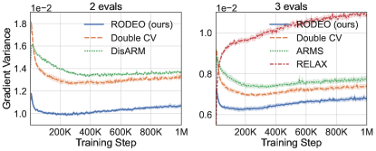
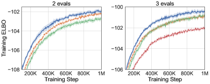
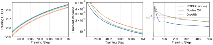
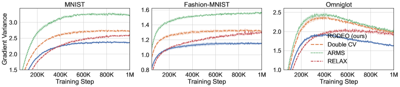
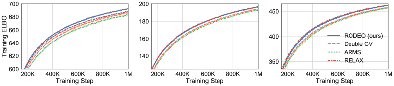
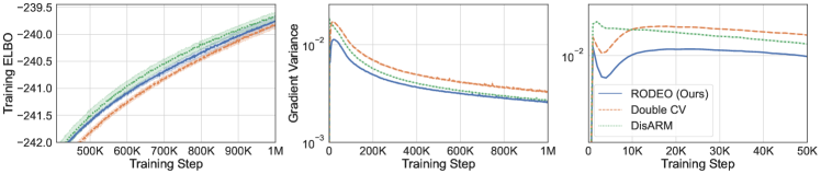
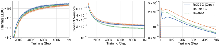
In the first set of experiments we focus on the most common setting of sample points and compare our variance reduction method to its counterparts including DisARM [14] and Double CV [60]. Results for RLOO are omitted since it is consistently outperformed by Double CV [see 60]. Table 2 shows, on all three datasets, RODEO achieves the best training ELBOs. In Figure 1 (left), we plot the gradient variance and average training ELBOs against training steps for all estimators on dynamically binarized MNIST. RODEO outperforms DisARM and Double CV by a large margin in gradient variance.
 |
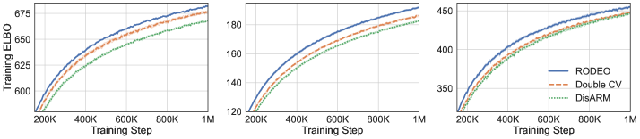 |
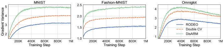
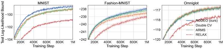
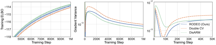
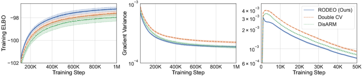
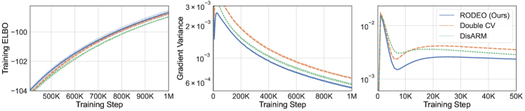
Next, we consider VAEs with Gaussian likelihoods trained on non-binarized datasets. In this case the gradient estimates suffer from even higher variance due to the large range of values can take. The results are plotted in Figure 2. We see that RODEO has substantially lower variance than DisARM and Double CV, leading to significant improvements in training ELBOs. In Appendix Figure 7, we find that RODEO also consistently yields the best test set performance in all six settings.
In the second set of experiments we compare RELAX [20], which uses three evaluations of per training step, with RODEO, Double CV, and ARMS [13] for . Figure 1 (right) and Table 2 demonstrate that RODEO outperforms the three previous methods and generally leads to the lowest variance. Although RELAX was often observed to have very strong performance in prior work [14, 60], our results in Figure 1 suggest that, for dynamically binarized datasets, much larger gains can be achieved by using the same number of function evaluations in other estimators.
For the experiments mentioned above, we report final training ELBOs in Table 2, test log-likelihood bounds in Appendix Table 4, and binarized MNIST average running time in Appendix Table 5. For , RODEO has the best final performance in 5 out of 6 tasks and runtime nearly identical to RELAX. For , RODEO has the best final performance for all tasks and is 1.5 times slower than Double CV and DisARM. We attribute the runtime gap to the Gibbs operator 4 which performs evaluations of the auxiliary functions and in 13 and 14. While this results in some extra cost, the network parameterizing and takes only 2-dimensional inputs, produces scalar outputs, and is typically small relative to the VAE model. As a result, the evaluation of and is significantly cheaper than that of , and its relative contribution to runtime shrinks as the cost of grows. To demonstrate this, we include a wall clock time comparison of our method with RLOO in Section C.1. In this experiment we replace the two-layer MLP-based VAE with a ResNet VAE, where the cost of is significantly higher than the single-layer MLP of . In this case, RODEO and RLOO have very close per-iteration time (0.025s vs. 0.023s). And RODEO achieves better training ELBOs than RLOO for the same amount of time.
6.2 Training hierarchical Bernoulli VAEs
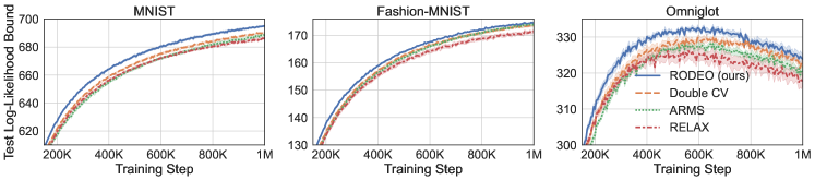
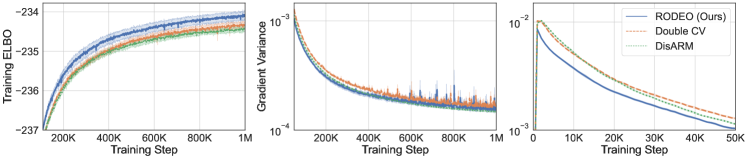
To investigate the performance of RODEO when scaling to hierarchical discrete latent variable models, we follow DisARM [14, 68] to train VAEs with 2/3/4 stochastic layers, each of which consists of Bernoulli variables. We set and compare our estimator with DisARM and Double CV on dynamically binarized MNIST, Fashion-MNIST, and Omniglot. For each stochastic layer, we use a different CV network which has the same architecture as those in our VAE experiments from the previous section. More details are presented in Appendix D.
 |
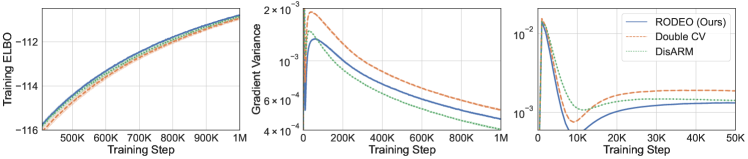
We plot the results on VAEs with four stochastic layers on Fashion-MNIST in Figure 3. The results for other datasets and for 2 and 3 stochastic layers can be found in Appendix E. RODEO generally achieves the best training ELBOs. One difference we noticed when comparing the variance results with those obtained from single-stochastic-layer VAEs is that these estimators have very different behaviors towards the beginning and the end of training. For example, in Figure 3, Double CV starts with lower variance than DisARM, but the gap diminishes after around 100K steps, and DisARM start to perform better as the training proceeds. In contrast, RODEO has the lowest variance in both phases for all datasets save Omniglot, where DisARM overtakes it in the long run.
6.3 Ablation study
Finally, we conduct an ablation study to gain more insight into the impact of each component of RODEO. In each experiment we train binary latent VAEs with .
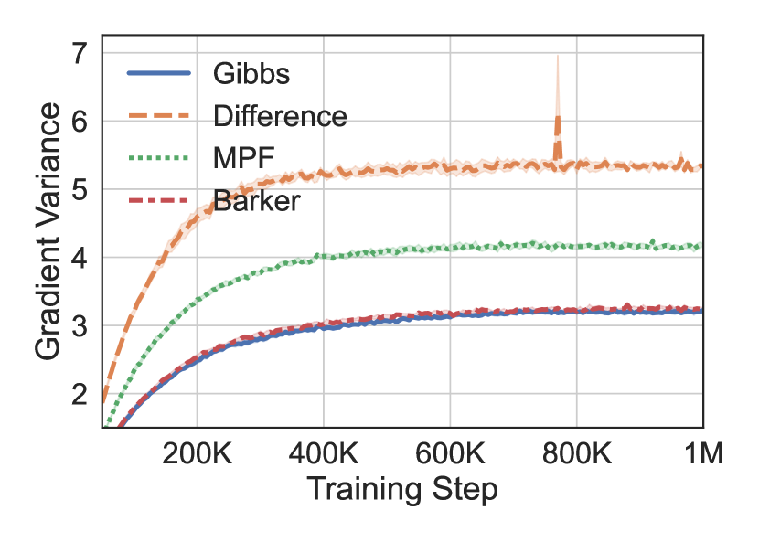
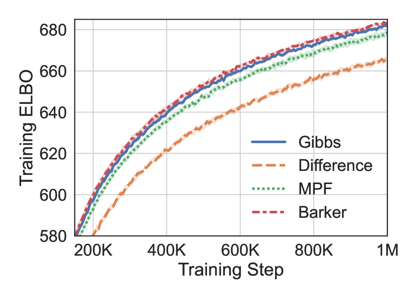
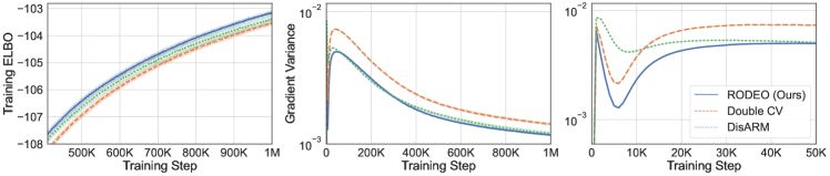
Impact of Stein operator Figure 4(a) explores the impact of RODEO Stein operator choice on non-binarized MNIST. As expected, the less stable difference 8 and MPF 6 operators lead to significantly higher gradient variances and worse training ELBOs. In fact, the same operators led to divergent training on binarized MNIST. The Barker operator 6 with neighborhoods defined by having one differing coordinate yields results very similar to Gibbs 4 as the operators themselves are very similar for binary variables (notice that when ).
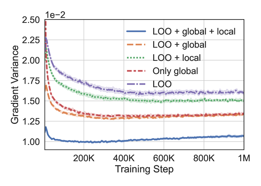
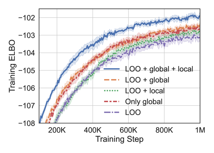
Impact of LOO baseline and global and local CVs Figure 4(b) explores binarized MNIST performance when RODEO is modified to retain a) only the LOO baseline (this is equivalent to standard RLOO), b) only the global CV, c) the LOO baseline + the global CV, or d) the LOO baseline + the local CV. We observe that the global and local Stein CVs both contribute to variance reduction and have complementary effects. Moreover, remarkably, the global Stein CV alone outperforms RLOO.
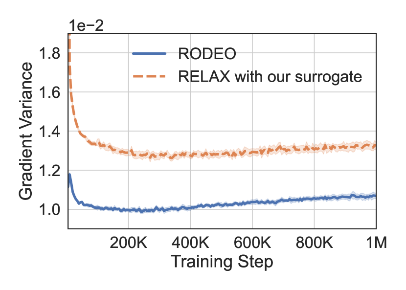
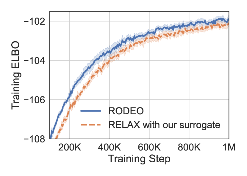
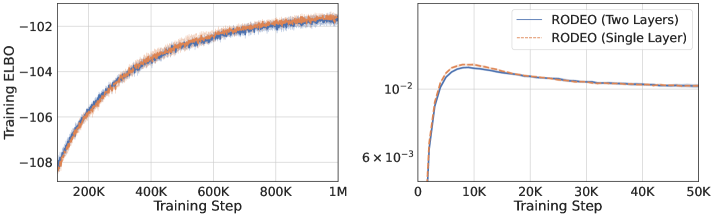
Impact of surrogate functions To tease apart the benefits of our new surrogate functions 13 and the remaining RODEO components, we replace the surrogate function in RELAX [20] with our surrogates, which only requires a single evaluation of per (see Appendix A for more details). Figure 4(c) compares the performance of RODEO and this modified RELAX on binarized MNIST. Since the surrogate functions are matched, the consistent improvements over modified RELAX can be attributed to the Stein and double CV components of RODEO. In Section C.2, we also experiment with increasing the complexity of and by using two hidden layers instead of a single hidden layer in the MLP. We did not observe significant improvements in variance reduction.
7 Conclusions, Limitations, and Future Work
This work tackles the gradient estimation problem for discrete distributions. We proposed a variance reduction technique which exploits Stein operators to generate control variates for REINFORCE leave-one-out estimators. Our RODEO estimator does not rely on continuous reparameterization of the distribution, requires no additional function evaluations per sample point, and can be adapted online to learn very flexible control variates parameterized by neural networks.
One potential drawback of our surrogate function constructions 13 and 14 is the need to evaluate an auxiliary function ( or ) at locations. This cost can be comfortably borne when and are much cheaper to evaluate than , such as in the ResNet VAE example in Section C.1 and many large VAE models used in practice [63]. And, in our experiments with the most common sample sizes, the runtime of RODEO was no worse than that of RELAX. To obtain a more favorable cost for large , one could employ alternative surrogates that require only a constant number of auxiliary function evaluations, e.g.,
The runtime of RODEO could also be improved by varying the Stein operator employed. For example, the Gibbs operator 4 used in our experiments evaluated its surrogate function at neighboring locations of . This evaluation complexity could be reduced by subsampling neighbors, resulting in a cheaper but still valid Stein operator, or by employing the numerically stable Barker operator 6 with fewer neighbors. Either strategy would introduce a speed-variance trade-off worthy of study in follow-up work. Finally, we have restricted our focus in this work to differentiable target functions . In future work, this limitation could be overcome by designing effective surrogate functions that make no use of derivative information.
Acknowledgments and Disclosure of Funding
We thank Heishiro Kanagawa for suggesting appropriate names for the Barker Stein operator.
References
- Anastasiou et al. [2021] Andreas Anastasiou, Alessandro Barp, François-Xavier Briol, Bruno Ebner, Robert E Gaunt, Fatemeh Ghaderinezhad, Jackson Gorham, Arthur Gretton, Christophe Ley, Qiang Liu, and Lester Mackey. Stein’s method meets statistics: A review of some recent developments. arXiv preprint arXiv:2105.03481, 2021.
- Assaraf and Caffarel [1999] Roland Assaraf and Michel Caffarel. Zero-variance principle for Monte Carlo algorithms. Phys. Rev. Lett., 83:4682–4685, Dec 1999.
- Barbour [1988] A. D. Barbour. Stein’s method and Poisson process convergence. J. Appl. Probab., (Special Vol. 25A):175–184, 1988. ISSN 0021-9002. A celebration of applied probability.
- Barker [1965] Av A Barker. Monte Carlo calculations of the radial distribution functions for a proton? electron plasma. Australian Journal of Physics, 18(2):119–134, 1965.
- Barp et al. [2018] Alessandro Barp, Chris Oates, Emilio Porcu, and Mark Girolami. A Riemann-Stein kernel method. arXiv preprint arXiv:1810.04946, 2018.
- Barp et al. [2019] Alessandro Barp, Francois-Xavier Briol, Andrew Duncan, Mark Girolami, and Lester Mackey. Minimum Stein discrepancy estimators. Advances in Neural Information Processing Systems, 32:12964–12976, 2019.
- Bengio et al. [2013] Yoshua Bengio, Nicholas Léonard, and Aaron Courville. Estimating or propagating gradients through stochastic neurons for conditional computation. arXiv preprint arXiv:1308.3432, 2013.
- Bresler and Nagaraj [2019] Guy Bresler and Dheeraj Nagaraj. Stein’s method for stationary distributions of Markov chains and application to Ising models. The Annals of Applied Probability, 29(5):3230–3265, 2019.
- Brown and Xia [2001] Timothy C. Brown and Aihua Xia. Stein’s Method and Birth-Death Processes. The Annals of Probability, 29(3):1373 – 1403, 2001.
- Burda et al. [2015] Yuri Burda, Roger Grosse, and Ruslan Salakhutdinov. Importance weighted autoencoders. International Conference on Learning Representations, 2015.
- Cong et al. [2019] Yulai Cong, Miaoyun Zhao, Ke Bai, and Lawrence Carin. GO gradient for expectation-based objectives. In International Conference on Learning Representations, 2019.
- Dellaportas and Kontoyiannis [2012] Petros Dellaportas and Ioannis Kontoyiannis. Control variates for estimation based on reversible Markov chain Monte Carlo samplers. Journal of the Royal Statistical Society: Series B (Statistical Methodology), 74(1):133–161, 2012.
- Dimitriev and Zhou [2021] Aleksandar Dimitriev and Mingyuan Zhou. ARMS: Antithetic-REINFORCE-Multi-Sample gradient for binary variables. In International Conference on Machine Learning, volume 139, pages 2717–2727, 2021.
- Dong et al. [2020] Zhe Dong, Andriy Mnih, and George Tucker. DisARM: An antithetic gradient estimator for binary latent variables. In Advances in Neural Information Processing Systems, volume 33, pages 18637–18647, 2020.
- Dong et al. [2021] Zhe Dong, Andriy Mnih, and George Tucker. Coupled gradient estimators for discrete latent variables. arXiv preprint arXiv:2106.08056, 2021.
- Eichelsbacher and Reinert [2008] Peter Eichelsbacher and Gesine Reinert. Stein’s method for discrete Gibbs measures. The Annals of Applied Probability, 18(4):1588–1618, 2008.
- Geyer [2011] Charles J. Geyer. Introduction to Markov chain Monte Carlo. In Steve Brooks, Andrew Gelman, Galin Jones, and Xiao-Li Meng, editors, Handbook of Markov Chain Monte Carlo, pages 3–48. CRC Press, 2011.
- Glynn [1990] Peter W. Glynn. Likelihood ratio gradient estimation for stochastic systems. Commun. ACM, 33(10):75–84, October 1990.
- Gorham and Mackey [2015] Jackson Gorham and Lester Mackey. Measuring sample quality with Stein’s method. In Advances in Neural Information Processing Systems, pages 226–234, 2015.
- Grathwohl et al. [2018] W. Grathwohl, D. Choi, Y. Wu, G. Roeder, and D. Duvenaud. Backpropagation through the void: Optimizing control variates for black-box gradient estimation. In International Conference on Learning Representations, 2018.
- Grathwohl et al. [2021] Will Grathwohl, Kevin Swersky, Milad Hashemi, David Duvenaud, and Chris Maddison. Oops I took a gradient: Scalable sampling for discrete distributions. In International Conference on Machine Learning, pages 3831–3841, 2021.
- Gu et al. [2016] Shixiang Gu, Sergey Levine, Ilya Sutskever, and Andriy Mnih. MuProp: Unbiased backpropagation for stochastic neural networks. In International Conference on Learning Representations, 2016.
- Henderson [1997] Shane G Henderson. Variance reduction via an approximating Markov process. PhD thesis, Stanford University, 1997.
- Hodgkinson et al. [2020] Liam Hodgkinson, Robert Salomone, and Fred Roosta. The reproducing stein kernel approach for post-hoc corrected sampling. arXiv preprint arXiv:2001.09266, 2020.
- Holmes [2004] Susan Holmes. Stein’s method for birth and death chains. In Persi Diaconis and Susan Holmes, editors, Stein’s Method: Expository Lectures and Applications, pages 42–65. 2004.
- Jang et al. [2017] Eric Jang, Shixiang Gu, and Ben Poole. Categorical reparameterization with Gumbel-softmax. International Conference on Learning Representations, 2017.
- Jankowiak and Obermeyer [2018] Martin Jankowiak and Fritz Obermeyer. Pathwise derivatives beyond the reparameterization trick. In International Conference on Machine Learning, pages 2235–2244. PMLR, 2018.
- Karlin and McGregor [1957] Samuel Karlin and James McGregor. The classification of birth and death processes. Transactions of the American Mathematical Society, 86(2):366–400, 1957.
- Kingma and Welling [2014] Diederik P. Kingma and Max Welling. Auto-encoding variational Bayes. In International Conference on Learning Representations, 2014.
- Kool et al. [2019] W. Kool, H. V. Hoof, and M. Welling. Buy 4 REINFORCE samples, get a baseline for free! In DeepRLStructPred@ICLR, 2019.
- Kool et al. [2020] Wouter Kool, Herke van Hoof, and Max Welling. Estimating gradients for discrete random variables by sampling without replacement. In International Conference on Learning Representations, 2020.
- Lake et al. [2015] Brenden M Lake, Ruslan Salakhutdinov, and Joshua B Tenenbaum. Human-level concept learning through probabilistic program induction. Science, 350(6266):1332–1338, 2015.
- LeCun et al. [1998] Yann LeCun, Léon Bottou, Yoshua Bengio, and Patrick Haffner. Gradient-based learning applied to document recognition. Proceedings of the IEEE, 86(11):2278–2324, 1998.
- Liu et al. [2017] Hao Liu, Yihao Feng, Yi Mao, Dengyong Zhou, Jian Peng, and Qiang Liu. Action-depedent control variates for policy optimization via Stein’s identity. arXiv preprint arXiv:1710.11198, 2017.
- Maddison et al. [2017] Chris J Maddison, Andriy Mnih, and Yee Whye Teh. The concrete distribution: A continuous relaxation of discrete random variables. In International Conference on Learning Representations, 2017.
- Mira et al. [2013] Antonietta Mira, Reza Solgi, and Daniele Imparato. Zero variance Markov chain Monte Carlo for Bayesian estimators. Statistics and Computing, 23(5):653–662, 2013.
- Mnih and Gregor [2014] Andriy Mnih and Karol Gregor. Neural variational inference and learning in belief networks. In International Conference on Machine Learning, pages 1791–1799, 2014.
- Mnih and Rezende [2016] Andriy Mnih and Danilo Rezende. Variational inference for Monte Carlo objectives. In International Conference on Machine Learning, pages 2188–2196, 2016.
- Mohamed et al. [2020] Shakir Mohamed, Mihaela Rosca, Michael Figurnov, and Andriy Mnih. Monte Carlo gradient estimation in machine learning. Journal of Machine Learning Research, 21(132):1–62, 2020.
- Niepert et al. [2021] Mathias Niepert, Pasquale Minervini, and Luca Franceschi. Implicit MLE: backpropagating through discrete exponential family distributions. Advances in Neural Information Processing Systems, 34:14567–14579, 2021.
- Oates et al. [2017] Chris J Oates, Mark Girolami, and Nicolas Chopin. Control functionals for Monte Carlo integration. Journal of the Royal Statistical Society: Series B (Statistical Methodology), 79(3):695–718, 2017.
- Owen [2013] Art B. Owen. Monte Carlo theory, methods and examples. 2013.
- Paisley et al. [2012] John Paisley, David M Blei, and Michael I Jordan. Variational Bayesian inference with stochastic search. In International Conference on Machine Learning, pages 1363–1370, 2012.
- Parmas and Sugiyama [2021] Paavo Parmas and Masashi Sugiyama. A unified view of likelihood ratio and reparameterization gradients. In International Conference on Artificial Intelligence and Statistics, pages 4078–4086. PMLR, 2021.
- Ranganath et al. [2014] Rajesh Ranganath, Sean Gerrish, and David Blei. Black box variational inference. In International Conference on Artificial Intelligence and Statistics, page 814–822, 2014.
- Reinert and Ross [2019] Gesine Reinert and Nathan Ross. Approximating stationary distributions of fast mixing Glauber dynamics, with applications to exponential random graphs. The Annals of Applied Probability, 29(5):3201–3229, 2019.
- Rezende et al. [2014] Danilo J. Rezende, Shakir Mohamed, and Daan Wierstra. Stochastic backpropagation and approximate inference in deep generative models. In International Conference on Machine Learning, 2014.
- Richter et al. [2020] Lorenz Richter, Ayman Boustati, Nikolas Nüsken, Francisco Ruiz, and Omer Deniz Akyildiz. VarGrad: A low-variance gradient estimator for variational inference. In Advances in Neural Information Processing Systems, volume 33, pages 13481–13492, 2020.
- Salimans and Knowles [2014] Tim Salimans and David A Knowles. On using control variates with stochastic approximation for variational Bayes and its connection to stochastic linear regression. arXiv preprint arXiv:1401.1022, 2014.
- Schulman et al. [2015] John Schulman, Nicolas Heess, Theophane Weber, and Pieter Abbeel. Gradient estimation using stochastic computation graphs. Advances in Neural Information Processing Systems, 28, 2015.
- Shazeer et al. [2017] Noam Shazeer, Azalia Mirhoseini, Krzysztof Maziarz, Andy Davis, Quoc Le, Geoffrey Hinton, and Jeff Dean. Outrageously large neural networks: The sparsely-gated mixture-of-experts layer. arXiv preprint arXiv:1701.06538, 2017.
- Si et al. [2020] Shijing Si, Chris Oates, Andrew B Duncan, Lawrence Carin, and François-Xavier Briol. Scalable control variates for Monte Carlo methods via stochastic optimization. arXiv preprint arXiv:2006.07487, 2020.
- Sohl-Dickstein et al. [2011] Jascha Sohl-Dickstein, Peter Battaglino, and Michael R DeWeese. Minimum probability flow learning. In International Conference on Machine Learning, pages 905–912, 2011.
- South et al. [2018] Leah F South, Chris J Oates, Antonietta Mira, and Christopher Drovandi. Regularised zero-variance control variates for high-dimensional variance reduction. arXiv preprint arXiv:1811.05073, 2018.
- Stein [1972] Charles Stein. A bound for the error in the normal approximation to the distribution of a sum of dependent random variables. In Proceedings of the Sixth Berkeley Symposium on Mathematical Statistics and Probability, Volume 2: Probability Theory. The Regents of the University of California, 1972.
- Stein et al. [2004] Charles Stein, Persi Diaconis, Susan Holmes, and Gesine Reinert. Use of exchangeable pairs in the analysis of simulations. Lecture Notes-Monograph Series, pages 1–26, 2004.
- Stirzaker [2005] David Stirzaker. Stochastic processes and models. OUP Oxford, 2005.
- Titsias and Lázaro-Gredilla [2014] Michalis K. Titsias and Miguel Lázaro-Gredilla. Doubly stochastic variational Bayes for non-conjugate inference. In International Conference on Machine Learning, 2014.
- Titsias and Lázaro-Gredilla [2015] Michalis K Titsias and Miguel Lázaro-Gredilla. Local expectation gradients for black box variational inference. Advances in neural information processing systems, 28:2638–2646, 2015.
- Titsias and Shi [2022] Michalis K Titsias and Jiaxin Shi. Double control variates for gradient estimation in discrete latent variable models. International Conference on Artificial Intelligence and Statistics, 2022.
- Tokui and Sato [2017] Seiya Tokui and Issei Sato. Evaluating the variance of likelihood-ratio gradient estimators. In International Conference on Machine Learning, pages 3414–3423, 2017.
- Tucker et al. [2017] G. Tucker, A. Mnih, C. J. Maddison, and J. Sohl-Dickstein. REBAR: Low-variance, unbiased gradient estimates for discrete latent variable models. In Advances in Neural Information Processing Systems, 2017.
- Vahdat and Kautz [2020] Arash Vahdat and Jan Kautz. NVAE: A deep hierarchical variational autoencoder. Advances in Neural Information Processing Systems, 33:19667–19679, 2020.
- Weaver and Tao [2001] Lex Weaver and Nigel Tao. The optimal reward baseline for gradient-based reinforcement learning. In Conference on Uncertainty in Artificial Intelligence, pages 538–545, 2001.
- Williams [1992] Ronald J Williams. Simple statistical gradient-following algorithms for connectionist reinforcement learning. Machine learning, 8(3-4):229–256, 1992.
- Xiao et al. [2017] Han Xiao, Kashif Rasul, and Roland Vollgraf. Fashion-MNIST: a novel image dataset for benchmarking machine learning algorithms. arXiv preprint arXiv:1708.07747, 2017.
- Yang et al. [2018] Jiasen Yang, Qiang Liu, Vinayak Rao, and Jennifer Neville. Goodness-of-fit testing for discrete distributions via Stein discrepancy. In International Conference on Machine Learning, pages 5561–5570. PMLR, 2018.
- Yin and Zhou [2019] Mingzhang Yin and Mingyuan Zhou. ARM: Augment-REINFORCE-merge gradient for stochastic binary networks. In International Conference on Learning Representations, 2019.
- Yin et al. [2020] Mingzhang Yin, Nhat Ho, Bowei Yan, Xiaoning Qian, and Mingyuan Zhou. Probabilistic best subset selection via gradient-based optimization, 2020.
- Zanella [2020] Giacomo Zanella. Informed proposals for local MCMC in discrete spaces. Journal of the American Statistical Association, 115(530):852–865, 2020.
Appendix A Sample-dependent Baselines in REBAR and RELAX
We start with the REINFORCE estimator with the sample-dependent baseline :
| (15) |
REBAR [62] introduces indirect independence on in through the continuous reparameterization , where is a continuous variable and is an argmax-like thresholding function. Specifically, , where is a continuous relaxation of controlled by the parameter . The correction term decomposes into two parts:
Both parts can be estimated with the reparameterization trick [29, 47, 58] which often has low variance. The RELAX [20] estimator generalizes REBAR by noticing that can be replaced with a free-form differentiable function . However, RELAX still relies on parameterizing as to achieve strong performance, as noted in Dong et al. [14].
To form modified RELAX in Section 6.3, we replace with for defined in 13.
Appendix B Proof of Unbiasedness of RODEO
Recall our estimator defined in RODEO is
| (16) |
To show the unbiasedness, we compute its expectation under as
Since the first term is the desired gradient and the third term is zero, it suffices to show that the second term also vanishes. Using the law of total expectations, we find for ,
which completes the proof.
Appendix C Additional Experiments
C.1 Wall clock time comparison with RLOO
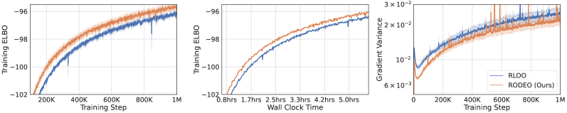
Besides necessary target function evaluations, the RODEO estimator comes with the additional cost of evaluating the neural network-based . Therefore, RODEO is most suited to the problems where the cost of evaluating dominates that of evaluating . This is often the case in practice. For example, state-of-the-art variational autoencoders [e.g., 63] are often built on expensive neural architectures such as deep residual networks (ResNets). Here, to demonstrate the practical advantage of our method as the complexity of grows, we replace the two-layer MLP VAEs used in previous experiments with a ResNet VAE (architecture shown in Table 3), while the neural network used by remains a single-layer MLP with 100 hidden units. We then compare the wall clock performance of RODEO with RLOO. The latent variables in this experiment remain binary and have 200 dimensions.
The results are shown in Figure 5. RODEO achieves better training ELBOs than RLOO in the same amount of time. In fact, for this VAE architecture, the per-iteration time of RODEO is 25.2ms, which is very close to the 23.1ms of RLOO. This indicates that the cost of is significantly higher than that of .
 |
| Encoder | Decoder |
| Conv 3x3x16, strides 1, padding 1 | Fully connected, 7x7x64 units |
| Conv Res block 3x3x16 | Deconv Res block 3x3x64 |
| Conv Res block 3x3x16 | Deconv Res block 3x3x64 |
| Conv Res block 3x3x32 (downsample by 2) | Deconv Res block 3x3x32 (upsample by 2) |
| Conv Res block 3x3x32 | Deconv Res block 3x3x32 |
| Conv Res block 3x3x64 (downsample by 2) | Deconv Res block 3x3x16 (upsample by 2) |
| Conv Res block 3x3x64 | Deconv Res block 3x3x16 |
| Fully connected, 200 units | Deconv 3x3x1, strides 1, padding 1 |
C.2 Impact of neural network architectures of surrogate functions
We conduct one more ablation study to investigate the impact of neural network architectures used by . Specifically, we replace the single-hidden-layer control variate network used in previous experiments with a two-hidden-layer MLP (each layer has 100 units) and compare their performance on binarized MNIST with . We keep other settings the same as in Section 6.1. The results are plotted in Figure 6. We do not observe significant difference between the two versions of RODEO.
 |
Appendix D Experimental Details
Our implementation is based on the open-source code of DisARM [14] (Apache license) and Double CV [60] (MIT license). Our figures display 1M training steps and our tables report performance after 1M training steps to replicate the experimental settings of DisARM [14].
D.1 Details of VAE experiments
VAEs are models with a joint density , where denotes the latent variable. is assigned a uniform factorized Bernoulli prior. The likelihood is parameterized by the output of a neural network with as input and parameters . The VAE has two hidden layers with units activated by LeakyReLU with the coefficient . To optimize the VAE we use Adam with base learning rate for non-binarized data and for dynamically binarized data, except for binarized Fashion-MNIST we decreased the learning rate to because otherwise the training is very unstable for all estimators. We use Adam with the same learning rate for adapting our control variate network in all experiments. The batch size is . The settings of other estimators are kept the same with Titsias and Shi [60].
In the minimum probability flow (MPF) and Barker Stein operator 6, we choose the neighborhood to be the states that differ in only one coordinate from . Let be an element in this neighborhood such that and . For the MPF Stein estimator and the difference Stein estimator 8, the density ratio can be simplified to . We further replace it with to alleviate numerical instability. The Barker Stein estimator does not suffer from the numerical issue since the coefficient is bounded in the Bernoulli case: . In our experiments, we find that the difference Stein estimator is highly unstable and may diverge as the iteration proceeds.
D.2 Details of hierarchical VAE experiments
We optimize the hierarchical VAE using Adam with base learning rate . Our control variate network is optimized using Adam with learning rate . Settings of training multilayer VAEs are kept the same with Dong et al. [14], except that we do not optimize the prior distribution of the VAE hidden layer and use a larger batch size .
Appendix E Additional Results
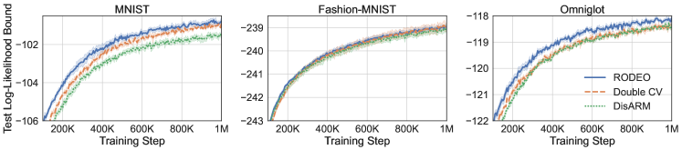
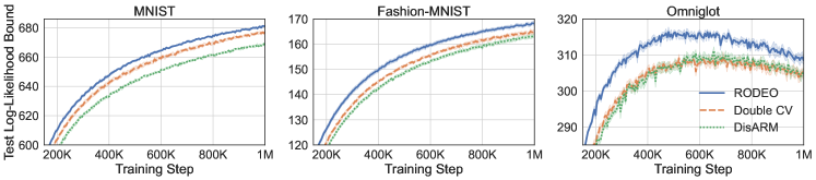
In this section, we measure test set performance using 100 test points and the marginal log-likelihood bound of Burda et al. [10], which provides a tighter estimate of marginal log likelihood than the ELBO. Throughout, we call this the “test log-likelihood bound.”
| Bernoulli Likelihoods | Gaussian Likelihoods | ||||||
| MNIST | Fashion-MNIST | Omniglot | MNIST | Fashion-MNIST | Omniglot | ||
| DisARM | |||||||
| Double CV | |||||||
| RODEO (Ours) | |||||||
| ARMS | |||||||
| Double CV | |||||||
| RODEO (Ours) | |||||||
| RELAX (3 evals) | |||||||
|
Binarized |
 |
|
Non-binarized |
 |
 |
 |
|
Binarized |
 |
|
Non-binarized |
 |
|
MNIST |
 |
|
Fashion-MNIST |
 |
|
Omniglot |
 |
|
MNIST |
 |
|
Fashion-MNIST |
 |
|
Omniglot |
 |
|
MNIST |
 |
|
Fashion-MNIST |
 |
|
Omniglot |
 |
| Double CV | DisARM/ARMS | RODEO (Ours) | RELAX (3 evals) | |
| 2.11 ms/step | 1.89 ms/step | 3.08 ms/step | 4.71 ms/step | |
| 2.28 ms/step | 1.91 ms/step | 4.72 ms/step |
| Double CV | DisARM | RODEO (Ours) | |
| Two layers | 4.33 ms/step | 3.54 ms/step | 6.79 ms/step |
| Three layers | 7.69 ms/step | 6.09 ms/step | 10.61 ms/step |
| Four layers | 11.67 ms/step | 9.53 ms/step | 14.91 ms/step |
| Training ELBO | Test Log-Likelihood Bound | ||||||
| MNIST | Fashion-MNIST | Omniglot | MNIST | Fashion-MNIST | Omniglot | ||
| Two layers | Double CV | ||||||
| DisARM | |||||||
| RODEO (Ours) | |||||||
| Three layers | Double CV | ||||||
| DisARM | |||||||
| RODEO (Ours) | |||||||
| Four layers | Double CV | ||||||
| DisARM | |||||||
| RODEO (Ours) | |||||||