\ul
Graph Contrastive Learning with
Cross-view Reconstruction
Abstract
Graph self-supervised learning is commonly taken as an effective framework to tackle the supervision shortage issue in the graph learning task. Among different existing graph self-supervised learning strategies, graph contrastive learning (GCL) has been one of the most prevalent approaches to this problem. Despite the remarkable performance those GCL methods have achieved, existing GCL methods that heavily depend on various manually designed augmentation techniques still struggle to alleviate the feature suppression issue without risking losing task-relevant information. Consequently, the learned representation is either brittle or unilluminating. In light of this, we introduce the Graph Contrastive Learning with Cross-View Reconstruction (GraphCV), which follows the information bottleneck principle to learn minimal yet sufficient representation from graph data. Specifically, GraphCV aims to elicit the predictive (useful for downstream instance discrimination) and other non-predictive features separately. Except for the conventional contrastive loss which guarantees the consistency and sufficiency of the representation across different augmentation views, we introduce a cross-view reconstruction mechanism to pursue the disentanglement of the two learned representations. Besides, an adversarial view perturbed from the original view is added as the third view for the contrastive loss to guarantee the intactness of the global semantics and improve the representation robustness. We empirically demonstrate that our proposed model outperforms the state-of-the-art on graph classification task over multiple benchmark datasets.
1 Introduction
Graph representation learning (GRL) has attracted significant attention due to its widespread applications in the real-world interaction systems, such as social, molecules, biological and citation networks (Hamilton et al., 2017b). The current state-of-the-art supervised GRL methods are mostly based on Graph Neural Networks (GNNs) (Kipf & Welling, 2017; Veličković et al., 2018; Hamilton et al., 2017a; Xu et al., 2019), which require a large amount of task-specific supervised information. Despite the remarkable performance, they are usually limited by the deficiency of label supervision in real-world graph data due to the fact that it is usually easy to collect unlabeled graph but very costly to obtain enough annotated labels, especially in certain fields like biochemistry. Therefore, many recent works (Qiu et al., 2020; Hassani & Khasahmadi, 2020a; Sun et al., 2019) study how to fully utilize the unlabeled information on graph and further stimulate the application of self-supervised learning (SSL) for GRL where only limited or even no label is needed.
As a prevalent and effective strategy of SSL, contrastive learning follows the mutual information maximization principle (InfoMax) (Veličković et al., 2019) to maximize the agreements of the positive pairs while minimizing that of the negative pairs in the embedding space. However, the graph contrastive learning paradigm guided by the InfoMax principle is insufficient to learn robust and transferable representation. State-of-the-art GCL methods (Qiu et al., 2020; Hassani & Khasahmadi, 2020a; You et al., 2020) usually rely on augmentor(s) (e.g., Identity, Subgraph Sampling, Node Dropping, Edge Removing and Attributes Masking.) applied to the anchor graph to generate a positive pair of graphs and . Then, the graph feature encoder will be trained to ensure the representation consistency within the positive pair, i.e., . Consequently, such training strategy is heavily dependent on the choice and strength of graph augmentation techniques. To be more specific, moderate graph augmentation will push encoders to capture redundant and biased information (Tschannen et al., 2019), which could inadvertently suppress the space of important predictive features and negatively affect the representation transferability via the so-called "shortcut" solution (Geirhos et al., 2020; Minderer et al., 2020). A more intuitively illustration is provided in the Figure 1 (a), where the shared part of the two augmentation view include both predictive information (the overlapping area with ) and non-predictive information (shadow area). Such optimization result usually yield lower contrastive loss, however, it has been empirically proved that the redundant information could lead to poor robustness (Robinson et al., 2021), especially under the out-of-distribution (OOD) setting (Ye et al., 2021). We provide a showcase example in Appendix A to illustrate the OOD scenario on graph learning task. On the other hand, overly aggressive augmentation may easily lead to another extreme where many predictive features are randomly dropped and the learned representation does not contain sufficient predictive information for downstream instance discrimination. Recent works (Suresh et al., 2021; Li et al., 2022; You et al., 2021) propose to use automated augmentations to extract the invariant rationale features (Wu et al., 2022b; a). These methods assume the most salient sub-structure (those are resistant to graph augmentation) is sufficient to make rational and correct label identification, and thereby implement trainable augmentation operations (e.g., edge deleting, node dropping) to strictly regularize the graph topological structure. Despite that these methods can alleviate the aforementioned feature suppression issue to some extent, they still suffer from inherent limitation. The harsh regularization may force the encoders focusing on the easy-learned "shallower" features (e.g. graph size and node degree), which might be helpful under certain domains but not necessarily for others (Bevilacqua et al., 2021), thus fail to guarantee stronger robustness. Therefore, the GCL methods guided with the saliency philosophy is not flexible enough to balance the representation sufficiency and robustness without the guidance of explicit domain knowledge. To reconcile the robustness and sufficiency of the learned representation, a method which can reduce redundant and biased information without sacrificing the sufficiency of the predictive graph features is in urgent need.
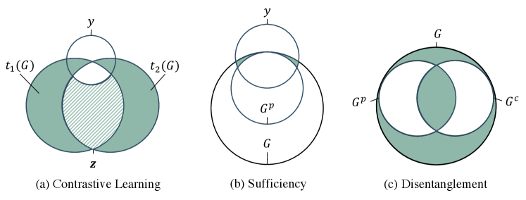
Recently, the information bottleneck (IB) principle (Tishby et al., 2000) has been introduced to the graph learning, which encourages extracting minimal yet sufficient information for representation learning. The core idea of IB principle is in accordance with the ultimate optimization objective to solve the feature suppression issue (Robinson et al., 2021), thus shed more light on this problem. Moreover, the representation learning guided by the IB principle has been empirically proved to generate more robust and transferable representations at different domains (Wu et al., 2020). Therefore, a graph contrastive learning framework in accordance with the IB principle is promising in balancing the representation robustness and sufficiency. Given an input graph , we denote and as its predictive feature subset and the complementary non-predictive feature subset, respectively. According to the assumption of recent studies about rationale invariance discover (Wu et al., 2022b; a), the two features subsets would the satisfy (sufficiency condition) and disentanglement condition (i.e., ). We illustrate the relations among the two feature subsets and in Figure 1 (b) and (c). It is inevitable that the learned representation maintains some redundant information for a specific downstream task. However, a GCL framework under the guidance of the IB principle is expected to suppress the feature space of as much as possible while keeping the predictive feature intact simultaneously in the learned representation.
In this paper, we propose the novel Graph Contrastive Learning with Cross-View Reconstruction, named GraphCV, to pursue the optimization objective of the IB principle. Specifically, GraphCV consists of a graph encoder followed with two decoders that are trained to extract information specific to the predictive and non-predictive features, respectively. To approximate the disentanglement objective, we propose the reconstruction-based representation learning scheme, including the intra-view and inter-view reconstructions, to reconstruct the original learned representation with the two separated feature subsets. Furthermore, the encoded representation from the original view perturbed in the adversarial fashion serves as the third view when computing the contrastive loss, apart from the predictive relevant representations of the two augmentation views, to further improve the representations’ robustness and prevent them from collapsing into partial or even trivial ones. We provide theoretical analysis to show that GraphCV is capable to learn minimal sufficient representations. Finally, we conduct experiments to validate the effectiveness of GraphCV over the commonly-used graph benchmark datasets. The experimental results demonstrate that GraphCV achieves significant performance gains over different datasets and settings compared with state-of-the-art baselines.
The main contributions of this work are summarized from three aspects: (i) We propose the GraphCV to alleviate the feature suppression issue with the cross-view reconstruction mechanism; (ii) We provide solid theoretical analysis on our model designs; (iii) Thorough experiments are conducted to demonstrate the robustness and transferability of the learned representations via GraphCV.
2 Preliminaries
2.1 Graph Representation Learning
In this work, we focus on the graph-level task, let denote a graph dataset with N graphs, where and are the node set and edge set of graph , respectively. We use and to denote the attribute vector of each node and edge . Each graph is associated with a label, denoted as , the goal the graph representation learning is to learn an encoder so that the learned representation is sufficient to predict related to the downstream task. We clarify the sufficiency of as containing no less information of the label of (Achille & Soatto, 2018), and it is formulated as:
| (1) |
where denotes the mutual information between two variables.
2.2 Contrastive Learning
Contrastive Learning (CL) is a self-supervised representation learning method which leverages instance-level identity for supervision. During the training phase, each graph firstly goes through proper data augmentation to generate two data augmentation views and , where and are two augmentation operators. Then, the CL method encourages the encoder (a backbone network plus a projection layer) to map and closer in the hidden space so that the learned representations and maintain all the information shared by and . The learning of the encoder is usually directed by a contrastive loss, such as NCE loss (Wu et al., 2018b), InfoNCE loss (van den Oord et al., 2018) and NT-Xent loss (Chen et al., 2020). In Graph Contrastive Learning (GCL), we usually adopt a GNN, such as GCN (Kipf & Welling, 2017) or GIN (Xu et al., 2019), as the backbone network, and the commonly-used graph data augmentation operators (You et al., 2020), such as node dropping, edge perturbation, subgraph sampling, and attribute masking.
All the GCL-based methods are built on the assumption that augmentations do not break the sufficiency requirement to make correct prediction. Here, we follow (Federici et al., 2020) to clear up the definition of mutual redundancy. is redundant to with respect of iff and share the same predictive information. Mathematically, the mutual redundancy in CL exists when:
| (2) |
Although GCL-based methods are usaully capable to extract useful information for label identification, it is unavoidable to include non-predictive features under the SSL setting owing lack of explicit domain knowledge. There exist the situation (e.g., OOD setting) that the latent space of learned representation is dominated by non-predictive features in SSL (Chen et al., 2021) and it is no more informative enough to make correct prediction. Therefore, feature suppression is not just a prevalent issue in supervised learning, but also in SSL. Due to the page limitation, we provide more discussion about the relation between feature suppression and GCL in Appendix B
3 Proposed Model
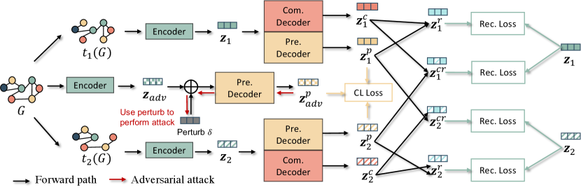
In this section, we introduce the details of our proposed GraphCV whose framework is shown in Figure 2. Corresponding theoretical analysis are provided to justify the rationality of our designs. Before diving into the details of GraphCV, we briefly introduce the overall framework of our model.
The proposed GraphCV model is designed in accordance with the IB principle to extract minimal yet sufficient representation through the designed cross-view reconstruction mechanism. Given as the graph encoder, we aim to map the graph representation into two different feature spaces , where is expected to be specific to the predictive information , and is optimized to elicit the complementary non-predictive factors . Later, we reconstruct the representation with the feature subsets mapped from same and different augmentation views to approximate the disentanglement objective demonstrated in Figure 1. By separating the learned representation into two sets of disentangled features and later utilizing them to reconstruct the two, we alleviate the feature suppression issue (Robinson et al., 2021) at no cost of information sufficiency. We further add extra regularization to guarantee does not collapse into shallow or partial features during the reconstruction process. We will introduce more details of GraphCV in the later contents.
3.1 Disentanglement by Cross-View Reconstruction
In GCL, we usually leverage a graph encoder, such as a GCN (Kipf & Welling, 2017) or a GIN (Xu et al., 2019), to encode the graph data into its representation. There are multiple choices of graph encoders in GCL, including GCN (Kipf & Welling, 2017) and GIN (Xu et al., 2019), etc. In this work, we adopt GIN as the backbone network for simplicity. Note that any other commonly-used graph encoders can also be adapted to our model. Given two augmentation views and (where and are IID sampled from the same family of augmentation ), we firstly use the encoder to map them into a lower dimension hidden space for the two embeddings, and . Instead of directly maximizing the agreement between the two representations and , we further feed each of them into a pair decoders , (both of them are MLP-based networks or GNN) and optimize the two decoders to map each of the presentation into the two disentangled feature sub-spaces:
| (3) |
where a pair of embeddings for both and are generated. Ideally, and suffice the mutual redundancy assumption stated in 2.2 because and are augmented from the same original graph, and thus naturally share the same predictive factors.
Here, we clarify the lower bound of the mutual information between one augmented view and the two mapped representations learned from the other augmented view in Theorem 1.
Theorem 1
Suppose is a GNN encoder as powerful as 1-WL test. Let and be specific to the predictive information of , meanwhile and account for the non-predictive factors of and . Then we have:
The detailed proof is provided in Appendix E. Given the lower bound, we substitute the objective by the mutual information between the two representations in the predictive view ( and ) to maximize the consistency between the information of the two views. Therefore, we derive the objective function ensuring view invariance as follows:
| (4) |
where is the adopted InfoNCE loss (van den Oord et al., 2018). To further pursue the feature disentanglement as illustrated in Figure 1(c), we thus propose the cross-view reconstruction mechanism. To be specific, we would like the representation pair within and cross the augmentation views be able to recover the raw data so that the two objectives can be approached simultaneously. Due to the fact that graphs are non-Euclidean structured data, we instead try to recover given and .
More specifically, we first perform the reconstruction within the augmentation view, namely mapping to , where representing the augmentation view. Then, we define the as a cross-view representation pair and the reconstruction procedure is repeated on it to predict , aiming to ensure and is optimized to approximate mutual disentanglement, where or . Intuitively, the reconstruction process is capable of separating the information of the shared features sets from the one resided in the unique feature sets between the two augmentation views. Since the two IID sampled augmentation operators ( and ) are expected to preserve the predictive/rational features while varying the augmentation-related ones, we disentangle the rational features from according to the rationale discover studies (Chang et al., 2020) to ensure the features’ robustness for downstream tasks. Here, we formulate the reconstruction procedures as:
| (5) |
where is the parameterized reconstruction model and is the free-to-choose fusion operator, such as element-wise product or concatenation. The reconstruction procedures are optimized by minimizing the entropy , where or . Ideally, we reach the optimal sufficiency and disentanglement conditions illustrated in Figure 1 (b) and (c) iff , where is exactly recovered given its complementary representation and the predictive representation of any view. Nevertheless, the condition probability is intractable, we hence use the variational distribution approximated by instead, denoted as . We provide the upper bound of in Theorem 2.
Theorem 2
Assume is a Gaussian distribution, is the parameterized reconstruction model which infers from . Then we have:
The detailed proof is demonstrated in Appendix E. Since we adopt two augmentation views, the objective function constraining representation disentanglement can be formulated as:
| (6) |
3.2 Adversarial Contrastive View
With the cross-view reconstruction mechanism above, the two learned representations stated above are optimized towards the disentangled manner. However, it is still necessary to further prevent the learned predictive representation from focusing on the partial features, because we do not have access to the explicit domain knowledge and such small scope will increase the risk of shortcut solution. Therefore, we extend the Equation 4 to three contrastive views and add an extra global view without topological perturbation as the third views to guarantee the learned maintain the global semantics instead of partial or even trivial features, i.e., and . During the experiments, we find an adversarial graph sample perturbed from original graph view can help the model achieve stronger robustness. A possible explanation is that there is still redundant information that is not predictive left in the shared information of the two ’s in the two augmentation views, especially when the implemented augmentations are moderate. An adversarial view may further alleviate redundancy. We define the adversarial objective as follows:
| (7) |
where the adversarial sample together with the two augmentation views, i.e., and are employed as the positive pair. Our crafted perturbation is spurred by recent work (Yang et al., 2021) that add perturbation on the output of first hidden layer , since it is empirically proved to generate more challenging views than adding perturbation on the initial node feature. Therefore, the adversarial contrastive objective is defined as:
| (8) |
where the optimized perturbation is solved by projected gradient descent (PGD) (Madry et al., 2018). Finally, we derive the joint objective of GraphCV by combining all of objectives above together. The joint objective is as follow:
| (9) |
where and are the coefficients to balance the magnitude of each loss term. Our proposed model is able to learn optimal representation illustrated in Figure 1(c) with the joint objective.
4 Experiments
In this section, we demonstrate the empirical evaluation results of GraphCV on public graph benchmark datasets under different settings. Ablation study and hyper-parameter analysis are also conducted to evaluate the effectiveness of the designs in GraphCV. We further compare the robustness of GraphCV with the adversarial training-based GCL method. More content about dataset statistics, training details and other empirical analysis are provided in the Appendix.
4.1 Experimental Setups
Datasets. For unsupervised learning setting, we evaluate our model on five graph benchmark datasets from the field of bioinformatics, including MUTAG, PTC-MR, NCI1, DD, and PROTEINS, and other four from the field of social network, which are COLLAB, IMDB-B, RDT-B, and IMDB-M, for the task of graph-level property classification. For the transfer learning setting, we follow previous work (You et al., 2020; Xu et al., 2021b) to pretrain our model on the ZINC-2M dataset, which cotains 2 million unlabeled molecule graphs sampled from MoleculeNet (Wu et al., 2018a), then evaluate its performance on eight binary classification datasets from chemistry domain, where the eight datasets are splitted according to the scaffold to simulate the out-of-distribution scenario in real-world. Additionally, We use ogbg-molhiv from Open Graph Benchmark Dataset (Hu et al., 2020a) to evaluate our model over large-scale dataset under semi-supervised setting. More details about dataset statistics are included in Appendix C.
Baselines. Under the unsupervised representation learning setting, we compare GraphCV with the eight SOTA self-supervised learning methods GraphCL (You et al., 2020), InfoGraph(Sun et al., 2019), MVGRL (Hassani & Khasahmadi, 2020a), AD-GCL(Suresh et al., 2021), GASSL(Yang et al., 2021), InfoGCL(Xu et al., 2021a), RGCL (Li et al., 2022) and DGCL(Li et al., 2021), as well as three classical unsupervised representation learning methods, including node2vec (Grover & Leskovec, 2016), graph2vec (Narayanan et al., 2017), and GVAE(Kipf & Welling, 2016). Besides, we employ AttrMasking (Hu et al., 2020b), ContextPred (Hu et al., 2020b), GraphCL (You et al., 2020), GraphLoG (Xu et al., 2021b), AD-GCL (Suresh et al., 2021) and RGCL (Li et al., 2022) as baselines to evaluate the effectiveness of our proposed GraphCV under transfer learning setting.
Evaluation Protocol. For unsupervised setting, we follow the evaluation protocols in the previous works (Sun et al., 2019; You et al., 2020; Li et al., 2021) to verify the effectiveness of our model. The mean test accuracy score evaluated by a 10-fold cross validation with standard deviation of five random seeds as the final performance. For transfer learning setting, we follow the finetuning procedures of previous work (You et al., 2020; Xu et al., 2021b) and report the mean ROC-AUC scores with standard deviation of 10 repeated runs on each downstream datasets. In addition, we follow the setting of semi-supervised representation learning from GraphCL on the ogbg-molhiv dataset, with the finetune label rates as 1%, 10%, and 20%. The final performance is reported as the mean ROC-AUC of five initialization random seeds
MUTAG PTC-MR COLLAB NCI1 PROTEINS IMDB-B RDT-B IMDB-M DD node2vec 72.6±10.2 58.6±8.0 - 54.9±1.6 57.5±3.6 - - - - graph2vec 83.2±9.3 60.2±6.9 - 73.2±1.8 73.3±2.1 71.1±0.5 75.8±1.0 50.4±0.9 - InfoGraph 89.0±1.1 61.7±1.4 70.7±1.1 76.2±1.1 74.4±0.3 73.0±0.9 82.5±1.4 49.7±0.5 72.9±1.8 VGAE 87.7±0.7 61.2±1.8 - - - 70.7±0.7 87.1±0.1 49.3±0.4 - MVGRL 89.7±1.1 62.5±1.7 - - - 74.2±0.7 84.5±0.6 51.2±0.5 - GraphCL 86.8±1.3 63.6±1.8 71.4±1.2 77.9±0.4 74.4±0.5 71.1±0.4 89.5±0.8 - 78.6±0.4 InfoGCL 91.2±1.3 63.5±1.5 80.0±1.3 80.2±0.6 - 75.1±0.9 - 51.4±0.8 - DGCL 92.1±0.8 65.8±1.5 81.2±0.3 81.9±0.2 76.4±0.5 75.9±0.7 91.8±0.2 51.9±0.4 - AD-GCL 89.7±1.0 - 73.3±0.6 69.7±0.5 73.8±0.5 72.3±0.6 85.5±0.8 49.9±0.7 75.1±0.4 RGCL 87.7±1.0 - 70.9±0.7 78.1±1.1 75.0±0.4 71.9±0.8 90.3±0.6 - 78.9±0.5 GASSL 90.9±7.9 64.6±6.1 78.0±2.0 80.2±1.9 - 74.2±0.5 - 51.7±2.5 - GraphCV 92.3±0.7 67.4±1.3 80.5±0.5 82.0±1.0 76.8±0.4 75.6±0.4 92.4±0.9 52.2±0.5 80.5±0.5
4.2 Overall Performance Comparison
Unsupervised learning. The overall performance comparison is shown in Table 1 and we can have three observations: (1) The GCL-based methods generally yield higher performances than classical unsupervised learning methods, indicating the effectiveness of utilizing instance-level supervision; (2) RGCL, AD-GCL, and GASSL achieve better performances than GraphCL, which empirically proves the conclusion that InfoMax object could bring overwhelmed redundant information and thus suffer from feature suppression issue; (3) Our proposed GraphCV and DGCL consistently outperform other baselines, proving the advantage of disentangled representation. More importantly, GraphCV achieves state-of-the-art results on most of the datasets, demonstrating the model effectiveness.
Transfer learning. Table 2 demonstrates the experimental results under transfer learning setting, where No Pre-Train skips self-supervised pre-training process on the ZINC-2M dataset for model initialization before finetune. It is noteworthy that some strong baselines (AttrMasking and ContextPred) are trained under the guidance of domain knowledge. Despite in lacking of such domain knowledge, our model still outperforms all the other baselines on 3 out 8 datasets and achieve highest average performance. More importantly, JOAO, RGCL and our proposed GraphCV are all developed from GraphCL, but achieve higher average performance than GraphCL. This observation further empirically prove the poisoning effect of biased information and the necessity to to suppress them.
BBBP Tox21 ToxCast SIDER ClinTox MUV HIV BACE Avg No Pre-Train 65.8±4.5 74.0±0.8 63.4 ±0.6 57.3±1.6 58.0±4.4 71.8±2.5 75.3±1.9 70.1±5.4 67.0 AttrMasking 64.3±2.8 76.7±0.4 64.2±0.5 61.0±0.7 71.8±4.1 74.7±1.4 77.2±1.1 79.3±1.6 71.1 ContextPred 68.0±2.0 75.7±0.7 63.9±0.6 60.9±0.6 65.9±3.8 75.8±1.7 77.3±1.0 79.6±1.2 70.9 GraphCL 69.5±0.5 75.4±0.9 63.8±0.4 60.8±0.7 70.1±1.9 74.5±1.3 77.6±0.9 78.2±1.2 70.8 GraphLoG 72.5±0.8 75.7±0.5 63.5±0.7 61.2±1.1 76.7±3.3 76.0±1.1 77.8±0.8 83.5±1.2 73.4 JOAO 70.2±1.0 75.0±0.3 62.9±0.5 60.0±0.8 81.3±2.5 71.7±1.4 76.7±1.2 51.5±0.4 71.9 RGCL 71.4±0.7 75.2±0.3 63.3±0.2 61.4±0.6 83.4 ±0.9 76.7 ±1.0 77.9±0.8 76.03±0.8 73.2 GraphCV 71.6±0.6 75.7±0.6 63.2±0.5 62.2±0.7 83.6±1.5 76.4±0.8 77.9±1.0 80.8±1.8 73.9
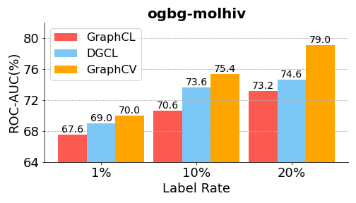
Semi-supervised learning. The experimental results are shown in Figure 3. It is obvious that our model gains significant improvements under the three label-rate fine-tuning settings. We also notice that as the label rate increases, the amount of improvement increases as well (1%, 1.8%, and 4.4% for label rate 1%, 10%, and 20%, respectively). A possible explanation could be that more trainable data could bring more redundant information, thereby further deteriorate the feature suppression issue. Therefore, removing redundant information causes a higher performance boost.
4.3 Ablation Study
To further verify the effectiveness of different modules in GraphCV, we perform ablation studies on each one of the module by creating two model variants: (1) w/o CV Recon, the cross-view reconstruction process is discarded; (2) w/o Adv. Training, the third adversarial view is discarded. The comparison results are shown in Table 3. We can observe from Table 3 that our model with the combination of cross-view reconstruction and adversarial training module outperforms all of the variants. Omitting the reconstruction process could cause the failure to optimize the representation in a disentangled manner illustrated in Figure 1(c), thereby the learned representation still suffer from features suppression issue. Compared with our model, the variant w/o Adv. Training may lead to representation collapse and bring extra redundant information, therefore resulting in sub-optimal performances in downstream tasks.
MUTAG PTC-MR COLLAB NCI1 PROTEINS IMDB-B RDT-B IMDB-M DD w/o CV Recon 91.0±0.9 64.7±1.4 78.0±0.8 78.7±1.2 74.9±0.7 75.0±0.6 91.1±0.7 51.7±0.6 79.0±0.8 w/o Adv. Training 92.1±0.6 66.8±0.5 76.5±0.6 81.2±0.9 76.0±0.3 75.1±0.6 92.2±1.0 50.8±0.4 80.1±0.6 GraphCV 92.3±0.7 67.4±0.5 80.5±0.5 82.0±1.0 76.8±0.4 75.6±0.4 92.5±0.9 52.2±0.5 80.5±0.5
4.4 Robustness and Hyper-parameter Analysis
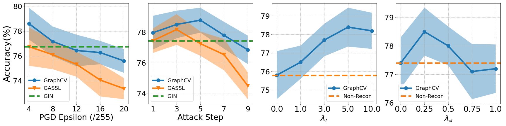
In this section, we firstly conduct extra experiments on ogbg-molhiv dataset to evaluate the representation robustness under aggressive augmentation and perturbation. The results are shown in left two subplots of Figure 4, we compare our method with GASSL under different perturbation bounds and attack steps to demonstrate its robustness against adversarial attacks. Since both our model and GASSL use GIN as the backbone network, we hereby add the performance of GIN as the compared baseline. Although aggressive adversarial attacks can largely deteriorate the performance, our proposed GraphCV still achieves more robust performance than GASSL. In the right two subplots, we analysis the model sensitivity of the two important hyper-parameters in our model, and . The consistent superiority of different values over the initial point (i.e., , ) prove the effectiveness of our design once again. We can also observe that the appropriate range of the two hyper-parameters are 5.0 to 10.0 and 0.0 to 0.5, respectively. Depend on the datasets size and attributes, the range can have some variance, we suggest to finetune the two hyper-parameters around 10.0 and 0.25 to find the appropriate values when adopting our model to a new datasets. More experiments and discussion about hyper-parameter sensitivity in provided in the Appendix H. Besides, we also conduct extra experiments to analyze the disentanglement of and in Appendix F.
5 Related Work
Graph contrastive learning. Contrastive learning is firstly proposed in the compute vision field (Chen et al., 2020) and raises a surge of interests in the area of self-supervised graph representation learning for the past few years. The principle behind contrastive learning is to utilize the instance-level identity as supervision and maximize the consistency between positive pairs in hidden space through designed contrast mode. Previous graph contrastive learning works generally rely on various graph augmentation (transformation) techniques (Veličković et al., 2019; Qiu et al., 2020; Hassani & Khasahmadi, 2020b; You et al., 2020; Sun et al., 2019) to generate positive pair from original data as similar samples. Recent works in this field try to improve the effectiveness of graph contrastive learning by finding more challenge view (Suresh et al., 2021; Xu et al., 2021a; You et al., 2021) or adding adversarial perturbation (Yang et al., 2021). However, most of the existing methods contrast over entangled embeddings, where the complex intertwined information may pose obstacles to extracting useful information for downstream tasks. Our model is spared from the issue by contrasting over disentangled representations.
Disentangled representation learning on graphs. Disentangled representation learning arises from the computer vision field (Hsieh et al., 2018; Zhao et al., 2021) to disentangle the heterogeneous latent factors of the representations, and therefore making the representations more robust and interpretable (Bengio et al., 2013). This idea has now been widely adopted in graph representation learning. (Liu et al., 2020; Ma et al., 2019) utilizes neighborhood routing mechanism to identify the latent factors in the node representations. Some other generative models (Kipf & Welling, 2016; Simonovsky & Komodakis, 2018) utilize Variational Autoencoders to balance reconstruction and disentanglement. Recent work (Li et al., 2021) outspreads the application of disentangled representations learning in self-supervised graph learning by contrasting the factorized representations. Although these methods gain significant benefit from the representation disentanglement, the underlined excessive information could still overload the model, thus resulting in limited capacities. Our model targets the issue by removing the redundant information that is considered irrelevant to the graph property.
Graph information bottleneck. The Information bottleneck (IB) (Tishby et al., 2000) has been widely adopted as a critical principle of representation learning. A representation contains minimal yet sufficient information is considered to be in compliance with the IB priciple and many works (Alemi et al., 2017; Shwartz-Ziv & Tishby, 2017; Federici et al., 2020) have empirically and theoretically proved that representation agree with IB principle is both informative and robust. Recently, IB principle is also borrowed to guide the representation learning of graph structure data. Current methods (Wu et al., 2020; Xu et al., 2021a; Suresh et al., 2021; Li et al., 2022) usually propose different regularization designs to learn compressed yet informative representations in accordance with IB principle. We follow the information bottleneck to learn the expressive and robust representation from disentangled information in this work.
6 Conclusion
In this paper, we study the feature suppression problem in representation learning. To avoid the predictive features being suppressed in learned representation, we propose a novel model, namely GraphCV, which is designed in accordance with the information bottleneck principle. The cross-view reconstruction in GraphCV can disentangle those more robust and transferable features from those easily-disturbed ones. Meanwhile, we also add an adversarial view as the third view of the contrastive learning to to guarantee the global semantics and further enhance representation robustness. In addition, we theoretically analyze the effectiveness of each component in our model and derive the objective based on the analysis. Extensive experiments on multiple graph benchmark datasets and different settings prove the ability of GraphCV to learn robust and transferable graph representation. In the future, we can explore how to come up with a practical objective to further decrease the upper bound of the mutual information between the disentangled representations and try to utilize more efficient training strategy to make the proposed model more time-saving on large-scale graphs.
Ethics Statement
This idea is proposed to solve the general graph learning problem, so we believe there should exist no ethical concern applicable to our work. Any unethical application that benefits from our work is against our initial intent.
Reproducibility Statement
We provide the source code along with the submission in the supplementary materials for reproducibility. The source code and all the implementation details will be open to public once upon the acceptance of this paper.
References
- Achille & Soatto (2018) Alessandro Achille and Stefano Soatto. Emergence of invariance and disentanglement in deep representations. JMLR, 2018.
- Alemi et al. (2017) Alexander A. Alemi, Ian Fischer, Joshua V. Dillon, and Kevin Murphy. Deep Variational Information Bottleneck. ICLR, 2017.
- Bengio et al. (2013) Yoshua Bengio, Aaron Courville, and Pascal Vincent. Representation Learning: A Review and New Perspectives. TPAMI, 2013. doi: 10.1109/TPAMI.2013.50.
- Bevilacqua et al. (2021) Beatrice Bevilacqua, Yangze Zhou, and Bruno Ribeiro. Size-invariant graph representations for graph classification extrapolations. In ICML, 2021.
- Chang et al. (2020) Shiyu Chang, Yang Zhang, Mo Yu, and Tommi Jaakkola. Invariant rationalization. In ICML, 2020.
- Chen et al. (2020) Ting Chen, Simon Kornblith, Mohammad Norouzi, and Geoffrey Hinton. A Simple Framework for Contrastive Learning of Visual Representations. In ICML, 2020. URL https://proceedings.mlr.press/v119/chen20j.html.
- Chen et al. (2021) Ting Chen, Calvin Luo, and Lala Li. Intriguing properties of contrastive losses. In NeurIPS, 2021.
- Cover (1999) Thomas M Cover. Elements of information theory. John Wiley & Sons, 1999.
- Federici et al. (2020) Marco Federici, Anjan Dutta, Patrick Forré, Nate Kushman, and Zeynep Akata. Learning robust representations via multi-view information bottleneck. In ICLR, 2020.
- Geirhos et al. (2020) Robert Geirhos, Jörn-Henrik Jacobsen, Claudio Michaelis, Richard Zemel, Wieland Brendel, Matthias Bethge, and Felix A Wichmann. Shortcut learning in deep neural networks. Nature Machine Intelligence, 2020.
- Grover & Leskovec (2016) Aditya Grover and Jure Leskovec. node2vec: Scalable Feature Learning for Networks. In KDD, 2016. URL https://doi.org/10.1145/2939672.2939754.
- Hamilton et al. (2017a) Will Hamilton, Zhitao Ying, and Jure Leskovec. Inductive Representation Learning on Large Graphs. In NeurIPS, 2017a. URL https://proceedings.neurips.cc/paper/2017/hash/5dd9db5e033da9c6fb5ba83c7a7ebea9-Abstract.html.
- Hamilton et al. (2017b) William L Hamilton, Rex Ying, and Jure Leskovec. Representation learning on graphs: Methods and applications. arXiv preprint arXiv:1709.05584, 2017b.
- Hassani & Khasahmadi (2020a) Kaveh Hassani and Amir Hosein Khasahmadi. Contrastive Multi-View Representation Learning on Graphs. In ICML, 2020a. URL https://proceedings.mlr.press/v119/hassani20a.html.
- Hassani & Khasahmadi (2020b) Kaveh Hassani and Amir Hosein Khasahmadi. Contrastive multi-view representation learning on graphs. In ICML, 2020b.
- Hsieh et al. (2018) Jun-Ting Hsieh, Bingbin Liu, De-An Huang, Li F Fei-Fei, and Juan Carlos Niebles. Learning to Decompose and Disentangle Representations for Video Prediction. In NeurIPS, 2018. URL https://proceedings.neurips.cc/paper/2018/hash/496e05e1aea0a9c4655800e8a7b9ea28-Abstract.html.
- Hu et al. (2020a) Weihua Hu, Matthias Fey, Marinka Zitnik, Yuxiao Dong, Hongyu Ren, Bowen Liu, Michele Catasta, and Jure Leskovec. Open Graph Benchmark: Datasets for Machine Learning on Graphs. In NeurIPS, 2020a. URL https://proceedings.neurips.cc/paper/2020/hash/fb60d411a5c5b72b2e7d3527cfc84fd0-Abstract.html.
- Hu et al. (2020b) Weihua Hu, Bowen Liu, Joseph Gomes, Marinka Zitnik, Percy Liang, Vijay Pande, and Jure Leskovec. Strategies for pre-training graph neural networks. In ICLR, 2020b.
- Kipf & Welling (2016) Thomas N. Kipf and Max Welling. Variational Graph Auto-Encoders. In NeurIPS, 2016.
- Kipf & Welling (2017) Thomas N. Kipf and Max Welling. Semi-Supervised Classification with Graph Convolutional Networks. In ICLR, 2017.
- Li et al. (2021) Haoyang Li, Xin Wang, Ziwei Zhang, Zehuan Yuan, Hang Li, and Wenwu Zhu. Disentangled Contrastive Learning on Graphs. In NeurIPS, 2021. URL https://openreview.net/forum?id=C_L0Xw_Qf8M.
- Li et al. (2022) Sihang Li, Xiang Wang, An Zhang, Xiangnan He, and Tat-Seng Chua. Let invariant rationale discovery inspire graph contrastive learning. In ICML, 2022.
- Liu et al. (2020) Yanbei Liu, Xiao Wang, Shu Wu, and Zhitao Xiao. Independence promoted graph disentangled networks. In AAAI, 2020.
- Ma et al. (2019) Jianxin Ma, Peng Cui, Kun Kuang, Xin Wang, and Wenwu Zhu. Disentangled Graph Convolutional Networks. In ICML, 2019. URL https://proceedings.mlr.press/v97/ma19a.html.
- Madry et al. (2018) Aleksander Madry, Aleksandar Makelov, Ludwig Schmidt, Dimitris Tsipras, and Adrian Vladu. Towards deep learning models resistant to adversarial attacks. In ICLR, 2018.
- Minderer et al. (2020) Matthias Minderer, Olivier Bachem, Neil Houlsby, and Michael Tschannen. Automatic shortcut removal for self-supervised representation learning. In ICML, 2020.
- Morris et al. (2020) Christopher Morris, Nils M. Kriege, Franka Bause, Kristian Kersting, Petra Mutzel, and Marion Neumann. TUDataset: A collection of benchmark datasets for learning with graphs. Technical report, arXiv, 2020. URL http://arxiv.org/abs/2007.08663.
- Narayanan et al. (2017) A. Narayanan, Mahinthan Chandramohan, R. Venkatesan, Lihui Chen, Yang Liu, and Shantanu Jaiswal. graph2vec: Learning Distributed Representations of Graphs. ArXiv, 2017.
- Qiu et al. (2020) Jiezhong Qiu, Qibin Chen, Yuxiao Dong, Jing Zhang, Hongxia Yang, Ming Ding, Kuansan Wang, and Jie Tang. GCC: Graph Contrastive Coding for Graph Neural Network Pre-Training. In KDD, 2020. ISBN 978-1-4503-7998-4. doi: 10.1145/3394486.3403168. URL https://doi.org/10.1145/3394486.3403168.
- Robinson et al. (2021) Joshua Robinson, Li Sun, Ke Yu, Kayhan Batmanghelich, Stefanie Jegelka, and Suvrit Sra. Can contrastive learning avoid shortcut solutions? In NeurIPS, 2021.
- Shwartz-Ziv & Tishby (2017) Ravid Shwartz-Ziv and Naftali Tishby. Opening the Black Box of Deep Neural Networks via Information. arXiv:1703.00810 [cs], April 2017. URL http://arxiv.org/abs/1703.00810.
- Simonovsky & Komodakis (2018) Martin Simonovsky and Nikos Komodakis. GraphVAE: Towards generation of small graphs using variational autoencoders. In ICLR, 2018.
- Sun et al. (2019) Fan-Yun Sun, Jordan Hoffmann, Vikas Verma, and Jian Tang. InfoGraph: Unsupervised and Semi-supervised Graph-Level Representation Learning via Mutual Information Maximization. In ICLR, 2019. URL http://arxiv.org/abs/1908.01000.
- Suresh et al. (2021) Susheel Suresh, Pan Li, Cong Hao, and Jennifer Neville. Adversarial Graph Augmentation to Improve Graph Contrastive Learning. In NeurIPS, 2021. URL https://proceedings.neurips.cc/paper/2021/hash/854f1fb6f65734d9e49f708d6cd84ad6-Abstract.html.
- Tishby et al. (2000) Naftali Tishby, Fernando C Pereira, and William Bialek. The information bottleneck method. arXiv preprint physics/0004057, 2000.
- Tschannen et al. (2019) Michael Tschannen, Josip Djolonga, Paul K Rubenstein, Sylvain Gelly, and Mario Lucic. On mutual information maximization for representation learning. In ICLR, 2019.
- van den Oord et al. (2018) Aaron van den Oord, Yazhe Li, and Oriol Vinyals. Representation Learning with Contrastive Predictive Coding. arXiv e-prints, 2018. URL https://ui.adsabs.harvard.edu/abs/2018arXiv180703748V.
- Veličković et al. (2018) Petar Veličković, Guillem Cucurull, Arantxa Casanova, Adriana Romero, Pietro Liò, and Yoshua Bengio. Graph Attention Networks. In ICLR, 2018. URL https://openreview.net/forum?id=rJXMpikCZ.
- Veličković et al. (2019) Petar Veličković, William Fedus, William L. Hamilton, Pietro Liò, Yoshua Bengio, and R. Devon Hjelm. Deep Graph Infomax. In ICLR, 2019. URL https://openreview.net/forum?id=rklz9iAcKQ.
- Wu et al. (2022a) Qitian Wu, Hengrui Zhang, Junchi Yan, and David Wipf. Handling distribution shifts on graphs: An invariance perspective. In ICLR, 2022a.
- Wu et al. (2020) Tailin Wu, Hongyu Ren, Pan Li, and Jure Leskovec. Graph Information Bottleneck. In NeurIPS. Curran Associates, Inc., 2020. URL https://proceedings.neurips.cc/paper/2020/hash/ebc2aa04e75e3caabda543a1317160c0-Abstract.html.
- Wu et al. (2022b) Ying-Xin Wu, Xiang Wang, An Zhang, Xiangnan He, and Tat seng Chua. Discovering invariant rationales for graph neural networks. In ICLR, 2022b.
- Wu et al. (2018a) Zhenqin Wu, Bharath Ramsundar, Evan N Feinberg, Joseph Gomes, Caleb Geniesse, Aneesh S Pappu, Karl Leswing, and Vijay Pande. Moleculenet: a benchmark for molecular machine learning. Chemical science, 9(2):513–530, 2018a.
- Wu et al. (2018b) Zhirong Wu, Yuanjun Xiong, Stella X. Yu, and Dahua Lin. Unsupervised Feature Learning via Non-Parametric Instance Discrimination. In CVPR, 2018b. URL https://openaccess.thecvf.com/content_cvpr_2018/html/Wu_Unsupervised_Feature_Learning_CVPR_2018_paper.html.
- Xu et al. (2021a) Dongkuan Xu, Wei Cheng, Dongsheng Luo, Haifeng Chen, and Xiang Zhang. InfoGCL: Information-Aware Graph Contrastive Learning. In NeurIPS, 2021a. URL https://proceedings.neurips.cc/paper/2021/hash/ff1e68e74c6b16a1a7b5d958b95e120c-Abstract.html.
- Xu et al. (2019) Keyulu Xu, Weihua Hu, Jure Leskovec, and Stefanie Jegelka. How Powerful are Graph Neural Networks? In ICLR, 2019. URL https://openreview.net/forum?id=ryGs6iA5Km.
- Xu et al. (2021b) Minghao Xu, Hang Wang, Bingbing Ni, Hongyu Guo, and Jian Tang. Self-supervised graph-level representation learning with local and global structure. In ICML, 2021b.
- Yang et al. (2021) Longqi Yang, Liangliang Zhang, and Wenjing Yang. Graph Adversarial Self-Supervised Learning. In NeurIPS, 2021. URL https://proceedings.neurips.cc/paper/2021/hash/7d3010c11d08cf990b7614d2c2ca9098-Abstract.html.
- Ye et al. (2021) Haotian Ye, Chuanlong Xie, Tianle Cai, Ruichen Li, Zhenguo Li, and Liwei Wang. Towards a theoretical framework of out-of-distribution generalization. In NeurIPS, 2021.
- You et al. (2020) Yuning You, Tianlong Chen, Yongduo Sui, Ting Chen, Zhangyang Wang, and Yang Shen. Graph Contrastive Learning with Augmentations. In NeurIPS, 2020. URL https://proceedings.neurips.cc/paper/2020/hash/3fe230348e9a12c13120749e3f9fa4cd-Abstract.html.
- You et al. (2021) Yuning You, Tianlong Chen, Yang Shen, and Zhangyang Wang. Graph contrastive learning automated. In ICLR, 2021.
- Zhao et al. (2021) Long Zhao, Yuxiao Wang, Jiaping Zhao, Liangzhe Yuan, Jennifer J. Sun, Florian Schroff, Hartwig Adam, Xi Peng, Dimitris Metaxas, and Ting Liu. Learning View-Disentangled Human Pose Representation by Contrastive Cross-View Mutual Information Maximization. In CVPR, 2021. URL https://openaccess.thecvf.com/content/CVPR2021/html/Zhao_Learning_View-Disentangled_Human_Pose_Representation_by_Contrastive_Cross-View_Mutual_Information_CVPR_2021_paper.html.
- Zhu et al. (2021) Yanqiao Zhu, Yichen Xu, Qiang Liu, and Shu Wu. An Empirical Study of Graph Contrastive Learning. arXiv.org, 2021.
Appendix A Out-of-distribution Scenario on Graph
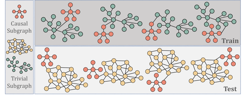
In this section, we will illustrate the out-of-distribution scenario in graph learning task. During molecule property study, A specific kind of property (e.g., toxicity and lipophilicity) of a molecule is usually dependent on if it has corresponding sub-structures (termed as functional group). For example, hydrophilic molecules usually have oxhydryl group () Therefore, a well-trained GNN model on molecule graph prediction task is capable to reflect the sub-structure information in the graph representation. However, it is usually the case in real-world scenario that the predictive functional group is usually accompanied by some irrelevant groups in some environments, thus causing spurious correlations. This correlation usually lead to poor generalization performance when the model is evaluated on another environment with different spurious correlation. Figure 5 intuitively demonstrates this kind of scenario, where the red subgraph is the feature we can rely on to make casual prediction. But it usually show up with green subgraph that do not serve as the functional graph of the property in training set. Consequently, the model are easily misguided that the green subgraph is an important indicator of the property. When we evaluate the model on the testing set where the casual graph is correlated with another kind of group (yellow subgraph), there usually exists a huge gap between its performances on the two sets.
Appendix B Discussion on Feature Suppression
In this section, we will follow the previous works (Chen et al., 2021; Robinson et al., 2021) to present a more formal definition of the feature suppression and clarify its relation with contrastive learning.
First of all, we assume graph data has feature sub-spaces, , where each corresponding to a distinct feature of . To quantify the relation between and its feature sub-spaces, we need to measure the conditional probability of given a specific kind of feature sub-space (), denoted as . Finally, we define a an injective map produce observation . Due to the reason that is not explicit, so we aim to train a encoder to map input graph data into a latent space to extract useful high-level information corresponding to each feature sub-space of input data during cotrastive learning. Therefore, we use as the approximated value of the measurement . Then we have,
-
•
For any feature sub-space and its complementary feature sub-subspace , suppress feature if we have
-
•
For any feature sub-space and its complementary feature sub-subspace , distinguish feature if and have disjoint support.
To sum up, a feature is suppressed if it does not make any difference to the instance discrimination. One of the common acknowledgements for unsuprevised learning strategy is that it can usually produce representation with uniform feature space distribution due to the lack of supervision, i.e., every feature sub-space is equally treated without feature suppression. However, it could not be the situation in contrastive learning. Taking the commonly used InfoNCE ](van den Oord et al., 2018) as an example, it can be divided into two parts, i.e. align term and uniform term (Chen et al., 2020), as follow:
| (10) |
Aligning the positive pair will distinguish the shared feature subspace . Meanwhile, there also exits random negative samples that might own same factors in , so the uniform term might suppress the feature sub-space . Therefore, for any feature , the optimization process can either suppress or distinguish it, but both of them can reach to lower contrastive loss. From the analysis we can derive the conclusion mentioned in Section 1 that lower contrastive loss might not yield better performance.
Appendix C Summary of Datasets
In this work, we use nine datasets from TU Benchmark Datasets (Morris et al., 2020) to evaluate our proposed GraphCV under unsupervised setting, where five of them are biochemical datasets and the other four belong to social network datasets. We also utilize the ogng-molhiv dataset from Open Graph Benchmark (OGB) (Hu et al., 2020a) to further evaluate GraphCV under semi-supervised setting. Besides, the datasets sampled from MoleculeNet (Wu et al., 2018a) are employed to evaluate our model under transfer learning setting. The statistics of these datasets are shown in Table 4 and 5.
| Dataset | #Graphs | Avg #Nodes | Avg #Edges | #Class | Metric | Category |
|---|---|---|---|---|---|---|
| MUTAG | 188 | 17.93 | 19.79 | 2 | Accuracy | biochemical |
| PTC-MR | 344 | 14.29 | 14.69 | 2 | Accuracy | biochemical |
| PROTEINS | 1,113 | 39.06 | 72.82 | 2 | Accuracy | biochemical |
| NCI1 | 4,110 | 29.87 | 32.30 | 2 | Accuracy | biochemical |
| DD | 1,178 | 284.32 | 715.66 | 2 | Accuracy | biochemical |
| COLLAB | 5,000 | 74.49 | 2457.78 | 3 | Accuracy | social network |
| IMDB-B | 1,000 | 19.77 | 96.53 | 2 | Accuracy | social network |
| RDT-B | 2,000 | 429.63 | 497.75 | 2 | Accuracy | social network |
| IMDB-M | 1,500 | 13.00 | 65.94 | 3 | Accuracy | social network |
| ogbg-molhiv | 41,127 | 25.50 | 27.50 | 2 | ROC-AUC | MoleculeNet |
| Dataset | #Graphs | Avg #Nodes | Avg Degree | #Tasks | Metric | Category |
|---|---|---|---|---|---|---|
| ZINC-2M | 2,000,000 | 26.62 | 57.72 | - | - | biochemical |
| BBBP | 2,039 | 24.06 | 51.90 | 1 | ROC-AUC | biochemical |
| Tox21 | 7,813 | 18.57 | 38.58 | 12 | ROC-AUC | biochemical |
| ToxCast | 8,576 | 18.78 | 38.62 | 617 | ROC-AUC | biochemical |
| SIDER | 1,427 | 33.64 | 70.71 | 27 | ROC-AUC | biochemical |
| ClinTox | 1,477 | 26.15 | 55.76 | 2 | ROC-AUC | biochemical |
| MUV | 93,087 | 24.23 | 52.55 | 17 | ROC-AUC | biochemical |
| HIV | 41,127 | 25.51 | 54.93 | 1 | ROC-AUC | biochemical |
| BACE | 1,513 | 34.08 | 73.71 | 1 | ROC-AUC | biochemical |
All of the eleven datasets are public available, we attach attach their links as follow:
-
•
TU datasets: https://chrsmrrs.github.io/datasets/docs/datasets/
-
•
MoleculeNet datasets: http://snap.stanford.edu/gnn-pretrain/
-
•
ogbg-molhiv dataset: https://ogb.stanford.edu/docs/graphprop/#ogbg-mol
Appendix D Implementation Details
All experiments are conducted with the following settings:
-
•
Operating System: Ubuntu 18.04.5 LTS
-
•
CPU: AMD(R) Ryzen 9 3900x
-
•
GPU: NVIDIA GeForce RTX 2080ti
-
•
Software: Python 3.8.5; Pytorch 1.10.1; PyTorch Geometric 2.0.4; PyGCL 0.1.2; Numpy 1.20.1; scikit-learn 0.24.1.
We implement our framework with PyTorch and PyGCL library (Zhu et al., 2021). We choose GIN (Xu et al., 2019) as the backbone graph encoder and the model is optimized through Adam optimizer. We choose GIN (Xu et al., 2019) as the backbone graph encoder and the model is optimized through Adam optimizer. We follow (You et al., 2020; Yang et al., 2021; Li et al., 2021) to employ a linear SVM classifier for downstream task-specific classification. The graph augmentation operations used in our work are same as (You et al., 2020), including node dropping, edge perturbation, attribute masking and subgraph sampling, all of them are borrowed from the implementation of (Zhu et al., 2021). There are two specific hyper-parameters in our model, namely and , the search space of them are and , respectively. For other important hyper-parameters, we find the best value of learning rate from , embedding dimension from , number of GNN layers from , batch size from (except for ogbg-molhiv ). Besides, we fix the perturbation bound , ascent step size and ascent step as 0.008, 0.008 and 5 during hyper-parameter fine-tuning. As for the implementation details of transfer learning, we basically follow the pre-training setting of previous works (You et al., 2020; Xu et al., 2021b).
Appendix E Proof
E.1 Proof of Theorem 1
We repeat Theorem 1 as follows.
Theorem 1. Suppose is a GNN encoder as powerful as 1-WL test. Let elicits only the augmentation information from meanwhile extracts the essential factors of from and . Then we have:
Proof. According to the assumption in Theorem 1, for any two graphs , if then we have , where and .
Besides, is specific to the predictive factors and is particular to the non-predictive factors, which means and are mutually excluded and . So we have,
| (11) |
Then, we want to prove that given three random variables , and , if they satisfy and , we have . According to the definition of mutual information, we have that,
| (12) | ||||
After that, by applying the chain rule to , we have,
| (13) | ||||
where is derived from the conclusion we get in Equation 12, is based on the non-negativity of mutual information, i.e., , and is because data processing inequality (Cover, 1999). Finally, we reach to the lower bound of in Equation 12, thus we can maximize the consistency between the information we capture from the two augmentation graph views by minimizing .
E.2 Proof of Theorem 2
We repeat Theorem 2 as follows.
Theorem 2. Assume is a Gaussian distribution, is the parameterized reconstruction model which infer from . Then we have:
Proof. To reconstruct the entangled representation from its corresponding non-predictive representation and the predictive representation of any augmentation view ( and are not necessarily equal), we need to minimize the conditional entropy:
| (14) |
Since the real distribution of is unknown and intractable, we hereby introduce a variational distribution to approximate it. Therefore, we have,
| (15) | ||||
Due to the non-negativity of KL-divergence between any two distributions, it is safe to say is the upper bound of . Based on the assumption of Theorem 2, let being a Gaussian distribution , where is the reconstruct network that predict from and is the variance. Thus we have,
| (16) | ||||
Hence, we get the upper bound of as Equation 16. To minimize the value of the unsolvable entropy, we can instead minimize the value of its upper bound and thereby derive the objective function as follow by neglecting the constant terms,
| (17) |
Since we adopt two augmentation views and propose the cross-view reconstruction mechanism in our method, we can minimize the entropy by minimizing and thus guarantee the disentanglement of and .
Appendix F Effects of Representation Disentanglement
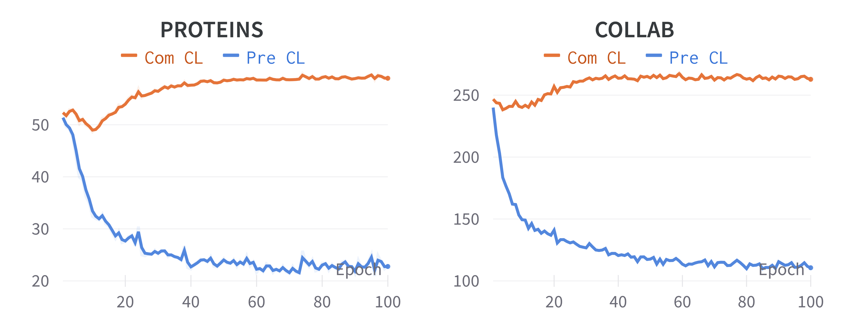
In this section, we set experiments to investigate the representation disentanglement of our proposed GraphCV. Specifically, we use the InfoNCE loss (van den Oord et al., 2018) to dynamically measure the representation difference between the two augmentation graph views based on the two disentangled representations, where blue lines indicate the InfoNCE loss between and and orange lines represent the InfoNCE loss between and . For simplicity, we only demonstrate the first 100 pre-training epochs of PROTEINS and COLLAB in Figure 6, we can observe similar phenomena on other datasets. From the loss curves in Figure 6 we can find that contrastive loss between predictive representations gradually decreases, indicating the predictive representation is optimized to capture all the shared information between the two augmentation view. Meanwhile, we can see contrastive loss between the non-predictive representations achieve a noticeable increases, which is consistent with our expectation that the two independent sampled augmentation operators cause a distribution shift between the two augmentation views. To further investigate whether the feature suppression problem is equally serious in and , we conduct experiments to compare the performance of the two representation on downstream tasks. The comparison results are as follow:
MUTAG COLLAB NCI1 PROTEINS IMDB-B RDT-B DD ogbg-molhiv 88.1±1.2 75.1±0.7 72.2±2.0 73.5±0.8 71.8±0.9 89.4±1.0 75.8±0.6 69.7.0±2.8 92.3±0.7 80.5±0.5 82.0±1.0 76.8±0.4 75.6±0.4 92.5±0.9 80.5±0.5 75.36±1.4
It is easily to observe that there is a obvious performance gap between the two learned representation, indicating the different feature suppression issue between them and the features subset that are more robust to augmentation is more informative and transferable that those sensitive to augmentations. Therefore, we believe our proposed GraphCV can further alleviate the feature suppression issue with the disentanglement design.
Appendix G Training Algorithm
In this sectionm we summarized the details of our proposed method in the following Algorithm.
Appendix H Hyper-parameter Sensitivity
In this section, we study the impacts of some important hyper-parameters in our method, including reconstruction loss coefficient , adversarial loss coefficient , embedding dimension , batch size and number of GNN layers . Here, we select four datasets, i.e., MUTAG, PROTEINS, RDT-B and COLLAB, to report for simplicity because the four datasets cover different domains and scales. We illustrate the impacts of these hyper-parameters in the figures below.
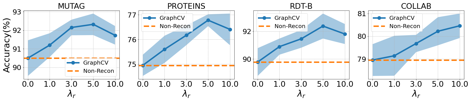
From the result demonstrated in Figure 7, we can see the optimal reconstruction loss coefficient is different dependent on the specific dataset, but all the values in our experiment can enhance the performance compared with non-reconstruction variant, i.e., , indicating the effectiveness of our proposed cross-view reconstruction mechanism.
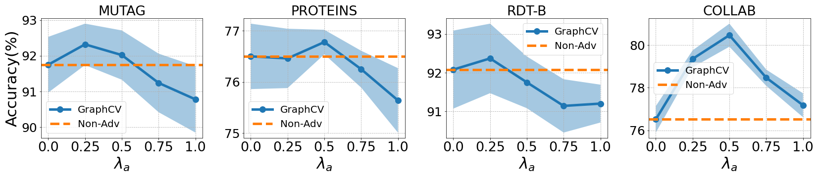
The Figure 8 shows that we could further raise the model performance through the adversarial training, which proves a robust representation with less redundant information usually achieve more performance gain compared with the brittle one. During this process, we need to choose a appropriate adversarial loss coefficient , otherwise a too large may hurt the information sufficiency of the learned representation.
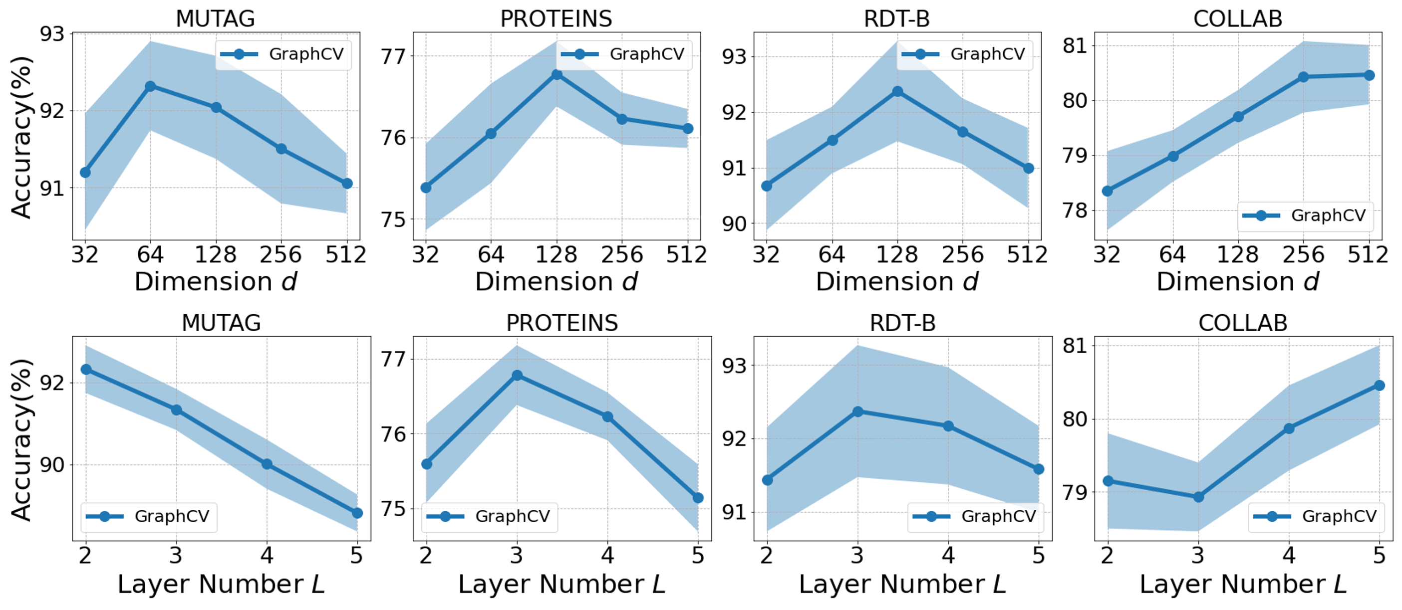
We put the impacts of embedding dimension and GNN layer number together because we can find a similar observation form their experimental results. From Figure 9, we observe that the optimal values of the two hyper-parameters generally increase as the dataset scale increases. The reason behind this phenomena could be large datasets usually contain more latent factors than the small datasets, therefore a model with larger capacity is needed to fit the large datasets. However, such high-capacity message-passing model will deteriorate the performance of small dataset because it may cause the learned representation over-smoothing and hence less informative.