Gravitational bremsstrahlung from spinning binaries
in the post-Minkowskian expansion

Consider the case of two spinning bodies approaching one another from infinity, and suppose that their distance of closest approach remains much larger than their individual radii. In this scenario, the details of their scattering encounter are well described by an EFT in which the two bodies are treated as point particles traveling along the worldlines of their respective centers of energy. Their dynamics are conveniently described by a Routhian [65, 105, 106, 107], which for each body of mass $m$ reads

The translational degrees of freedom (d.o.f.s) of this body are encoded in four worldline coordinates $x^{\mu}(\tau)$, which chart the integral curve of the four-velocity ${\mathcal{U}^{\mu}\equiv\text{d}x^{\mu}/\text{d}\tau}$. Only three of these are needed to specify the position of the body uniquely, however, and so we remove the remaining unphysical d.o.f. by imposing the constraint ${\mathcal{U}_{\mu}\mathcal{U}^{\mu}=1}$ [43, 65]. Meanwhile, the body’s rotational d.o.f.s are encoded in the antisymmetric spin tensor $\mathcal{S}_{ab}$, which notably is defined in a locally flat frame with coordinates $\{y^{a}\}$. Tensors defined in the general coordinate frame $\{x^{\mu}\}$ are transformed into the former by way of the vielbein ${e_{\mu}^{a}\equiv\partial y^{a}/\partial x^{\mu}}$ (e.g., ${\mathcal{U}^{a}\equiv e^{a}_{\mu}\mathcal{U}^{\mu}}$), which also defines for us the spin connection ${\omega_{\mu}^{ab}\coloneq g^{\rho\sigma}\!e^{b}_{\sigma}\nabla_{\!\mu}^{\vphantom{a}}e^{a}_{\rho}}$. Only three of the six components in $\mathcal{S}_{ab}$ are needed to specify the spin of the body uniquely; hence, the other three d.o.f.s are to be removed by imposing a spin supplementary condition (SSC) [108, 109, 110, 111]. Given the relativistic nature of the problem, the covariant SSC, ${\,\mathcal{U}^{a}\mathcal{S}_{ab}=0+O(\mathcal{S}^{3})}$ [111], proves to be the most convenient choice.

The first three terms in Eq. (1) are universal, in the sense that they apply to any body with a mass monopole and spin dipole. Higher-order multipole moments, however, are sensitive to the body’s internal structure, and this is why the final term in Eq. (1), which describes the self-induced quadrupole moment of the rotating body (${E_{\mu\nu}\equiv R_{\mu\rho\nu\sigma}\mathcal{U}^{\rho}\mathcal{U}^{\sigma}}$), is accompanied by the Wilson coefficient $C_{E}$. Kerr black holes have ${C_{E}=1}$ [106], although this value can be larger for objects like neutron stars [112, 113]. Infinitely many more terms can be appended to Eq. (1) should we wish to include even higher-order multipoles [114], or other finite-size effects like tidal deformations [115, 74], but these all come with higher powers of either the curvature tensors or the spin, and so are irrelevant to our purposes here.

As the Routhian behaves like a Lagrangian from the point of view of the translational d.o.f.s, but like a Hamiltonian with regards to the rotational d.o.f.s, the equations of motion for each body follow from a mixture of Euler-Lagrange and Hamilton equations [116]; namely,

The only nontrivial Poisson bracket we require is [105]

where $\eta^{ab}$ is the Minkowski metric with a mostly minus signature. Note that the aforementioned constraints on $\mathcal{U}^{\mu}$ and $\mathcal{S}_{ab}$ should be imposed only after all functional derivatives and Poisson brackets have been evaluated.

To fully specify our EFT, we must also endow the metric $g_{\mu\nu}$ with its own dynamics; hence, we take the full effective action to be ${S=S_{\text{EH}}+S_{\text{FP}}+\sum_{A=1}^{2}\int\text{d}\tau_{A}\mathcal{R}_{A}}$, where $S_{\text{EH}}$ is the Einstein-Hilbert action, $S_{\text{FP}}$ is a Faddeev-Popov term that enforces the de Donder gauge, and the label ${A\in\{1,2\}}$ is used to distinguish between the binary’s two constituents.

As a precursor to computing the radiated four-momentum, we first determine the stress-energy tensor $T^{\mu\nu}$ for the binary as a whole. This object is sourced by the multipolar moments of the two bodies, as well as by the energy stored in nonlinear interactions of the gravitational field, and can be obtained perturbatively from our EFT with the help of Feynman diagrams once we expand the action in powers of ${\kappa h_{\mu\nu}\coloneq g_{\mu\nu}-\eta_{\mu\nu}}$, with ${\kappa\equiv\sqrt{32\pi G}}$. Crucially, since

in this expansion, Greek and Latin indices are now indistinct. The spin tensors are, nonetheless, still defined in their respective locally flat frames [65].

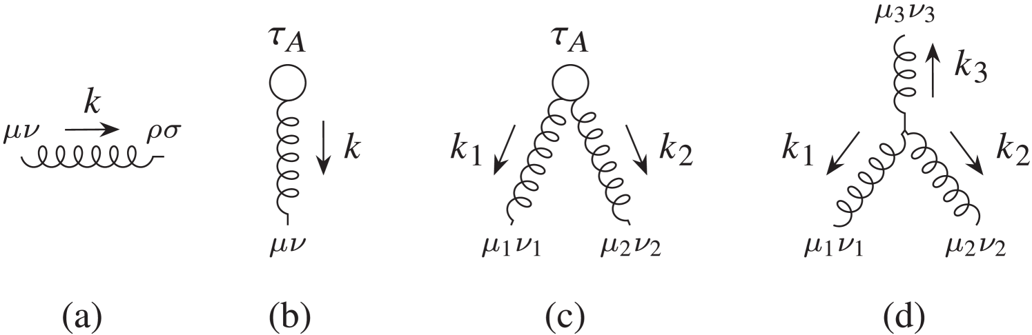
Only the Feynman rules shown in Fig. 1 are required at the order in $G$ to which we are working. In $d$-dimensional momentum space (we work in $d$ dimensions for added generality), the graviton propagator in Fig. 1(a) is $iP_{\mu\nu\rho\sigma}/k^{2}$, with ${P_{\mu\nu\rho\sigma}=\eta_{\mu(\rho}\eta_{\sigma)\nu}+\eta_{\mu\nu}\eta_{\rho\sigma}/(d-2)}$ (an $i\epsilon$ prescription is unnecessary at this order because the loop integrals never hit the poles at ${k^{2}=0}$ [83]), while the worldline vertex for single-graviton emission is

Expressions for the two remaining vertices, which are much lengthier, are presented in the Supplemental Material [104].

In addition to making the weak-field expansion above, we must also expand the body variables ${X_{A}\equiv(x_{A},\mathcal{U}_{A},\mathcal{S}_{A})}$ about their initial straight-line trajectories in order to achieve manifest power counting in $G$. We therefore write [43, 65]

where $\delta^{(n)}X_{A}$ is the $O(G^{n})$ deflection away from the initial trajectory $\overline{X}_{A}$ due to the gravitational pull of the other body. The 1PM deflections $\delta^{(1)}X_{A}$, which we will need later in our calculation, were previously computed using Eq. (2) in Refs. [43, 65]. (They are reproduced in the Supplemental Material [104] for completeness.) As for $\overline{X}_{A}$, we write

where the constant vectors $u_{A}^{\mu}$ and $b_{A}^{\mu}$ are the initial velocity and orthogonal displacement of the $A$th body, respectively, while the constant tensor $s_{A}^{\mu\nu}$ describes its initial spin per unit mass. Note that ${s_{A}^{\mu\nu}u_{A\,\nu}=0}$ as per the covariant SSC, while the impact parameter ${b^{\mu}_{\mathstrut}\coloneq b_{1}^{\mu}-b_{2}^{\mu}}$ satisfies ${b\cdot u_{A}=0}$ [43].

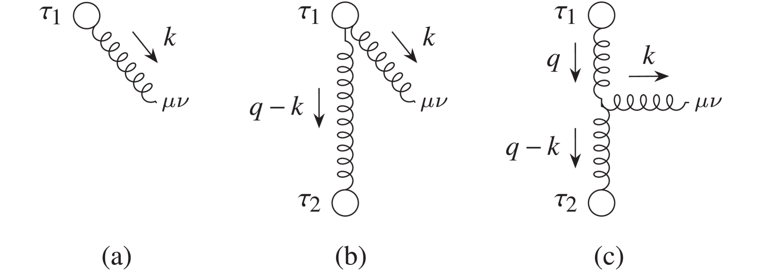
We now use these rules to compute the (tree-level) expectation value ${{\langle h_{\mu\nu}(k)\rangle}\equiv\kappa P_{\mu\nu\rho\sigma}T^{\rho\sigma}(k)/(2k^{2})}$, from which the (classical) stress-energy tensor $T^{\mu\nu}$ may be extracted. At leading order in $G$, only the diagram in Fig. 2(a), with $X_{A}$ replaced by $\overline{X}_{A}$, contributes. The result is

where the delta function ${\text{\smash{\raisebox{2.58334pt}{--}}\kern-4.73611pt$\delta$}(x)\equiv 2\pi\delta(x)}$ comes from having performed the integral over $\tau_{A}$ in Eq. (5).

All three diagrams in Fig. 2 contribute at next-to-leading order in $G$. From Fig. 2(a), we extract the $O(G)$ part of the diagram by expanding $X_{A}$ up to 1PM, whereas for Figs. 2(b) and 2(c), it suffices to replace $X_{A}$ by $\overline{X}_{A}$. The total result is

where ${M=m_{1}+m_{2}}$ is the binary’s total mass, ${\nu=m_{1}m_{2}/M^{2}}$ is its symmetric mass ratio, ${\int_{q}\!\equiv\!\int\text{d}^{d}q/(2\pi)^{d}}$, and $\Delta_{12}(q,k)\coloneq\,\text{\smash{\raisebox{2.58334pt}{--}}\kern-4.73611pt$\delta$}(q\cdot u_{1})\,\text{\smash{\raisebox{2.58334pt}{--}}\kern-4.73611pt$\delta$}((k-q)\cdot u_{2})$. An explicit expression for the object $t^{\mu\nu}$, accurate to $O(s^{2})$, is presented in the Supplemental Material [104].

Given the above, we may now compute the radiated four-momentum via the definition [117]

where ${\text{\smash{\raisebox{2.58334pt}{--}}\kern-4.73611pt$\delta$}_{+}(k^{2})\,\text{d}^{d}k/(2\pi)^{d}}$ is the Lorentz-invariant phase-space measure for the emission of on shell gravitons. Observe that because the delta functions in Eq. (8) have compact support away from ${k^{2}=0}$, $T^{\mu\nu}_{\text{LO}}$ is nonradiative and so does not contribute to $P^{\mu}_{\text{rad}}$. It therefore suffices to substitute Eq. (9) into Eq. (10) when working to leading order in $G$. We then find

Next, we define new momentum variables ${q=q_{1}-q_{2}}$, ${\ell_{1}=-q_{2}}$, and ${\ell_{2}=q_{1}-k}$ [73] in order to write

The radiated four-momentum may thus be viewed as the inverse Fourier transform of some object $Q^{\mu}$, which is expressible as a sum of terms in which $q^{\mu}$, $u_{A}^{\mu}$, and $s_{A}^{\mu\nu}$ are contracted amongst themselves and with the two-loop integrals

Following Ref. [90], we define $\rho_{2}={-2\ell_{1}\cdot u_{2}}$, $\rho_{3}={-2\ell_{2}\cdot u_{1}}$, ${\rho_{5}=\ell_{1}^{2}}$, ${\rho_{6}=\ell_{2}^{2}}$, ${\rho_{8}=(\ell_{1}-q)^{2}}$, and ${\rho_{9}=(\ell_{2}-q)^{2}}$, while the underlined variables are used to denote the presence of delta functions; i.e., ${2/\underline{\rho}{}_{1}=\text{\smash{\raisebox{2.58334pt}{--}}\kern-4.73611pt$\delta$}(\ell_{1}\cdot u_{1})}$, ${2/\underline{\rho}{}_{4}=\text{\smash{\raisebox{2.58334pt}{--}}\kern-4.73611pt$\delta$}(\ell_{2}\cdot u_{2})}$, and ${1/\underline{\rho}{}_{7}=\text{\smash{\raisebox{2.58334pt}{--}}\kern-4.73611pt$\delta$}_{+}(k^{2})}$ with ${k\equiv q-\ell_{1}-\ell_{2}}$. All of the integrals in $Q^{\mu}$ have $n_{1}=n_{4}={n_{7}=1}$. Reverse unitarity then allows us to treat these delta functions as cut propagators [91, 92, 93, 94].

The tensor-valued nature of these integrals make them cumbersome to evaluate as is, but fortunately they can all be reduced to scalar-valued ones via a suitable basis decomposition [85]. Specifically, we expand each of the loop momenta $\ell_{A}^{\mu}$ (${A\in\{1,2\}}$) in the numerator as

where ${\check{u}_{1}^{\mu}\coloneq(u_{1}^{\mu}-\gamma u_{2}^{\mu})/(1-\gamma^{2})}$ and ${\check{u}_{2}^{\mu}\!\coloneq\check{u}_{1}^{\mu}|_{1\leftrightarrow 2}}$ are the dual vectors to the two initial velocities (${\check{u}_{A}\cdot u_{B}=\delta_{AB}}$), ${\gamma\equiv u_{1}\cdot u_{2}}$ is the Lorentz factor for the relative velocity $v$, and $\ell_{A\bot}^{\mu}$ is the part of $\ell_{A}^{\mu}$ that is orthogonal to $u_{1}$, $u_{2}$, and $q$ [the delta functions in Eq. (12) guarantee that ${q\cdot u_{A}=0}$]. The three inner products in Eq. (14) are then easily rewritten in terms of the variables $\rho_{i}$ and $q^{2}$ only.

As for $\ell_{A\bot}^{\mu}$, the fact that the denominator of Eq. (13) is invariant under $(\ell_{1\bot},\ell_{2\bot})\mapsto-(\ell_{1\bot},\ell_{2\bot})$ implies that any term in the numerator with $i$ powers of $\ell_{1\bot}$ and $j$ powers of $\ell_{2\bot}$ will integrate to zero if ${i+j}$ is odd. If instead ${i+j=2}$, then rotational invariance on the hypersurface orthogonal to $u_{1}$, $u_{2}$, and $q$ allows us to replace

under the integral, where the metric on this hypersurface is ${\bot^{\mu\nu}=\eta^{\mu\nu}-\check{u}_{1}{}^{\mu}u_{1}{}^{\nu}-\check{u}_{2}{}^{\mu}u_{2}{}^{\nu}-q^{\mu}q^{\nu}/q^{2}}$, and note that the inner product ${(\ell_{A}^{\mathstrut\rho}\bot_{\rho\sigma}\ell_{B}^{\mathstrut\sigma})}$ is easily rewritten solely in terms of the variables $\rho_{i}$, $q^{2}$, and $\gamma$. Analogous replacement rules can be derived for the ${i+j=4}$ case by positing the ansatz $\ell_{A\bot}^{\mathstrut\mu}\ell_{B\bot}^{\mathstrut\nu}\ell_{C\bot}^{\mathstrut\rho}\ell_{D\bot}^{\mathstrut\sigma}\mapsto{c_{1}\bot^{\mu\nu}\bot^{\rho\sigma}}+{c_{2}\bot^{\mu\rho}\bot^{\nu\sigma}}+{c_{3}\bot^{\mu\sigma}\bot^{\rho\nu}}$ and then solving for the coefficients ${\{c_{1},c_{2},c_{3}\}}$ by taking appropriate contractions. The same can be done for all ${i+j\in 2\mathbb{Z}}$, although in practice we encounter only integrals with ${i+j\leq 5}$.

The object $Q^{\mu}$ is now a sum of terms in which different combinations of $q^{\mu}$, $u_{A}^{\mu}$, and $s_{A}^{\mu\nu}$ are contracted with one another and multiplied by one of the scalar-valued integrals $G_{n_{1}\cdots\,n_{9}}$. At this stage, $3100$ different scalar integrals enter into $Q^{\mu}$, but not all of them are independent. After using the LiteRed software package [118, 119] to identify nontrivial integration by parts relations between the different integrals [95, 96, 97], we find that they reduce to a set of only four master integrals; the same four as in Eqs. (4.13)–(4.16) of Ref. [73]. These are solved via differential equation methods [98, 99, 100, 101, 102, 103]; see Ref. [73] for details.

All that remains is to compute the Fourier transform in Eq. (12). We do so by using another family of master integrals,

whose scalar-valued member evaluates to

with ${\bot_{12}^{\mu\nu}=\eta^{\mu\nu}_{\mathstrut}-\check{u}_{1}^{\mathstrut\mu}u_{1}^{\mathstrut\nu}-\check{u}_{2}^{\mathstrut\mu}u_{2}^{\mathstrut\nu}}$ [67]. Its tensor-valued cousins follow from differentiation; e.g., ${I^{\mu}_{n}=-i\partial I_{n}/\partial b_{\mu}}$.

Now specializing to four dimensions, it becomes convenient to decompose our final result into components along the basis vectors $\{u_{1},u_{2},\hat{b},\hat{l}\}$, where ${\hat{b}^{\mu}\coloneq b^{\mu}/b}$ ${(b\equiv\sqrt{-b_{\mu}b^{\mu}})}$ and ${\hat{l}_{\mu}\coloneq\epsilon_{\mu\nu\rho\sigma}u_{1}^{\mathstrut\nu}u_{2}^{\mathstrut\rho}\hat{b}^{\mathstrut\sigma}_{\mathstrut}/\sqrt{\gamma^{2}-1}}$ are the unit vectors pointing along the impact parameter and orbital angular momentum, respectively. After also eliminating the spin tensors in favor of the Pauli-Lubanski spin vectors ${s_{A}^{\mu}\coloneq\epsilon^{\mu}_{\mathstrut}{}_{\nu\rho\sigma}u_{A}^{\mathstrut\nu}s_{A}^{\mathstrut\rho\sigma}/2}$, we find that we can write

The components $\mathcal{C}_{V}$, with ${V\in\{u_{1},u_{2},\hat{b},\hat{l}\}}$, are dimensionless functions of only the Lorentz factor $\gamma$, the two Wilson coefficients $C_{E_{A}}$, and the six inner products $(s_{A}\cdot V)/b$. (There are only six because ${s_{A}\cdot u_{A}=0}$ by definition.)

The fact that $P^{\mu}_{\text{rad}}$ is a polar vector strongly constrains which inner products can appear at any given order, and in which combinations. For instance, because $\mathcal{C}_{u_{1}}$, $\mathcal{C}_{u_{2}}$, and $\mathcal{C}_{\hat{b}}$ must all be even under parity, they can only depend on $(s_{A}\cdot\hat{l})/b$ at linear order in the spins. Indeed, we find explicitly that

while ${\mathcal{C}_{\hat{b}}=0+O(s^{2})}$. The remaining component $\mathcal{C}_{u_{2}}$ can be obtained from $\mathcal{C}_{u_{1}}$ by swapping the body labels ${1\leftrightarrow 2}$, since $P^{\mu}_{\text{rad}}$ must be symmetric under this interchange. As an added consequence, $\mathcal{C}_{\hat{b}}$ and $\mathcal{C}_{\hat{l}}$ must be odd and even under this interchange, respectively.

The four functions ${\{f_{\text{I}},\,\dots,f_{\text{IV}}\}}$ in Eq. (19) depend purely on $\gamma$ and are presented in Table 1 [$f_{\text{I}}$, which appears at $O(s^{0})$, was previously determined in Refs. [70, 71, 72, 73], but is reproduced here for completeness]. An additional 21 functions of $\gamma$, with similar analytic structures, appear at $O(s^{2})$. These are presented in the Supplemental Material [104]. Notice that $\mathcal{C}_{\hat{b}}$ and $\mathcal{C}_{\hat{l}}$ both vanish when the spins are aligned along $\hat{l}$ (or, indeed, when they are zero); hence, for so-called “aligned-spin” configurations, for which the binary’s motion is confined to a plane, we see that momentum is lost only in the direction of the relative velocity.

To validate Eq. (18) against the existing literature, we compare results for the energy $\Delta E$ radiated in the center-of-mass frame. This is computed in our approach as ${\Delta E=(P_{\text{rad}}\cdot p_{\text{tot}})/E}$, where ${p^{\mu}_{\text{tot}}=m_{1}^{\mathstrut}u_{1}^{\mu}+m_{2}^{\mathstrut}u_{2}^{\mu}}$ and ${E^{2}=p_{\text{tot}}^{2}=M^{2}[1+2\nu(\gamma-1)]}$. Since $\hat{b}^{\mu}$ and $\hat{l}^{\mu}$ are purely spatial in this frame, ${s_{A}\cdot\hat{b}}$ and ${s_{A}\cdot\hat{l}}$ are equivalent to the three-dimensional dot products ${-\,\mathbf{s}_{A}\cdot\hat{\vphantom{b}}\kern-1.4pt\mathbf{b}}$ and ${-\,\mathbf{s}_{A}\cdot\hat{\mathbf{l}}}$, respectively, and note that ${s_{1}\cdot u_{2}\simeq\mathbf{s}_{1}\cdot\mathbf{v}}$ while ${s_{2}\cdot u_{1}\simeq-\,\mathbf{s}_{2}\cdot\mathbf{v}}$ after expanding to first order in the relative 3-velocity $\mathbf{v}$. Having done so, our result for $\Delta E$ agrees with that of Ref. [85], which is accurate to leading order in $\mathbf{v}$ and to quadratic order in the spins, once we also replace $(\mathbf{b},\mathbf{s}_{A},C_{E_{A}})\mapsto(-\mathbf{b},-\mathbf{s}_{A},1-C_{E_{A}})$ to account for differing conventions.

As a second consistency check, we use analytic continuation by way of the boundary-to-bound (B2B) map [15, 16, 17] to convert our result for $\Delta E$ into the energy $\Delta E_{\text{ell}}$ radiated during one period of ellipticlike motion. This is accomplished in three steps. Owing to current limitations of the B2B map, we first specialize to aligned-spin configurations. Next, we must transform from the covariant SSC to the canonical (Newton-Wigner) SSC [110] for the map to work. This generally entails transforming $(\mathbf{b},\mathbf{s}_{A})$ to new canonical variables $(\mathbf{b}_{\text{c}},\mathbf{s}_{A\,\text{c}})$ [59, 60], but ${\mathbf{s}_{A}\equiv\mathbf{s}_{A\,\text{c}}}$ in the aligned-spin case; hence, only the magnitude of the impact parameter must be transformed. The rule is

where ${p_{\infty}=M^{2}\nu\sqrt{\gamma^{2}-1}/E}$ is the initial momentum of either body in the center-of-mass frame, ${a_{\pm}=(\mathbf{s}_{1}\!\pm\mathbf{s}_{2})\cdot\hat{\mathbf{l}}}$, and we may define ${L_{\text{c}}=b_{\text{c}}p_{\infty}}$ as the canonical orbital angular momentum. Finally, we obtain $\Delta E_{\text{ell}}$ from $\Delta E$ via [17]

having eliminated $\gamma$ in favor of ${\mathcal{E}\equiv(E-M)/(M\nu)}$. The left-hand side follows after analytic continuation from positive to negative values of $\mathcal{E}$. Expanded in powers of $\mathcal{E}$, we find that our result, which is valid in the large-angular-momentum limit [17], agrees with the overlapping terms from PN theory up to 3PN in Ref. [17], and up to 4PN in Refs. [120, 121].

References

- Abbott et al. [2016a] B. P. Abbott et al. (LIGO Scientific and Virgo Collaborations), Observation of Gravitational Waves from a Binary Black Hole Merger, Phys. Rev. Lett. 116, 061102 (2016a), arXiv:1602.03837.
- Abbott et al. [2017] B. P. Abbott et al. (LIGO Scientific and Virgo Collaborations), GW170817: Observation of Gravitational Waves from a Binary Neutron Star Inspiral, Phys. Rev. Lett. 119, 161101 (2017), arXiv:1710.05832.
- Berti et al. [2015] E. Berti et al., Testing general relativity with present and future astrophysical observations, Classical Quantum Gravity 32, 243001 (2015), arXiv:1501.07274.
- Abbott et al. [2021] R. Abbott et al. (LIGO Scientific and Virgo Collaborations), Tests of general relativity with binary black holes from the second LIGO-Virgo gravitational-wave transient catalog, Phys. Rev. D 103, 122002 (2021), arXiv:2010.14529.
- Barausse et al. [2020] E. Barausse et al., Prospects for fundamental physics with LISA, Gen. Relativ. Gravit. 52, 81 (2020), arXiv:2001.09793.
- Auclair et al. [2022] P. Auclair et al., Cosmology with the Laser Interferometer Space Antenna, arXiv:2204.05434.
- Arun et al. [2022] K. G. Arun et al., New horizons for fundamental physics with LISA, Living Rev. Relativity 25, 4 (2022), arXiv:2205.01597.
- Barausse [2012] E. Barausse, The evolution of massive black holes and their spins in their galactic hosts, Mon. Not. R. Astron. Soc. 423, 2533 (2012), arXiv:1201.5888.
- Callister et al. [2020] T. Callister, M. Fishbach, D. Holz, and W. Farr, Shouts and Murmurs: Combining individual gravitational-wave sources with the stochastic background to measure the history of binary black hole mergers, Astrophys. J. Lett. 896, L32 (2020), arXiv:2003.12152.
- Vitale et al. [2014] S. Vitale, R. Lynch, J. Veitch, V. Raymond, and R. Sturani, Measuring the Spin of Black Holes in Binary Systems Using Gravitational Waves, Phys. Rev. Lett. 112, 251101 (2014), arXiv:1403.0129.
- Abbott et al. [2016b] T. D. Abbott et al. (LIGO Scientific and Virgo Collaborations), Improved Analysis of GW150914 Using a Fully Spin-Precessing Waveform Model, Phys. Rev. X 6, 041014 (2016b), arXiv:1606.01210.
- Abbott et al. [2020] R. Abbott et al. (LIGO Scientific and Virgo Collaborations), GW190412: Observation of a binary-black-hole coalescence with asymmetric masses, Phys. Rev. D 102, 043015 (2020), arXiv:2004.08342.
- Blanchet [2014] L. Blanchet, Gravitational radiation from post-Newtonian sources and inspiralling compact binaries, Living Rev. Relativity 17, 2 (2014), arXiv:1310.1528.
- Damour [2016] T. Damour, Gravitational scattering, post-Minkowskian approximation, and effective-one-body theory, Phys. Rev. D 94, 104015 (2016), arXiv:1609.00354.
- Kälin and Porto [2020a] G. Kälin and R. A. Porto, From boundary data to bound states, J. High Energy Phys. 01 (2020) 072, arXiv:1910.03008.
- Kälin and Porto [2020b] G. Kälin and R. A. Porto, From boundary data to bound states. Part II. Scattering angle to dynamical invariants (with twist), J. High Energy Phys. 02 (2020) 120, arXiv:1911.09130.
- Cho et al. [2022a] G. Cho, G. Kälin, and R. A. Porto, From boundary data to bound states. Part III. Radiative effects, J. High Energy Phys. 04 (2022) 154, arXiv:2112.03976.
- Bini et al. [2020a] D. Bini, T. Damour, and A. Geralico, Sixth post-Newtonian nonlocal-in-time dynamics of binary systems, Phys. Rev. D 102, 084047 (2020a), arXiv:2007.11239.
- Damour [2018] T. Damour, High-energy gravitational scattering and the general relativistic two-body problem, Phys. Rev. D 97, 044038 (2018), arXiv:1710.10599.
- Bini and Damour [2017] D. Bini and T. Damour, Gravitational spin-orbit coupling in binary systems, post-Minkowskian approximation, and effective one-body theory, Phys. Rev. D 96, 104038 (2017), arXiv:1709.00590.
- Bini and Damour [2018] D. Bini and T. Damour, Gravitational spin-orbit coupling in binary systems at the second post-Minkowskian approximation, Phys. Rev. D 98, 044036 (2018), arXiv:1805.10809.
- Damour [2020a] T. Damour, Classical and quantum scattering in post-Minkowskian gravity, Phys. Rev. D 102, 024060 (2020a), arXiv:1912.02139.
- Antonelli et al. [2019] A. Antonelli, A. Buonanno, J. Steinhoff, M. van de Meent, and J. Vines, Energetics of two-body Hamiltonians in post-Minkowskian gravity, Phys. Rev. D 99, 104004 (2019), arXiv:1901.07102.
- Khalil et al. [2022] M. Khalil, A. Buonanno, J. Steinhoff, and J. Vines, Energetics and scattering of gravitational two-body systems at fourth post-Minkowskian order, Phys. Rev. D 106, 024042 (2022), arXiv:2204.05047.
- Neill and Rothstein [2013] D. Neill and I. Z. Rothstein, Classical space–times from the S-matrix, Nucl. Phys. B877, 177 (2013), arXiv:1304.7263.
- Bjerrum-Bohr et al. [2014] N. E. J. Bjerrum-Bohr, J. F. Donoghue, and P. Vanhove, On-shell techniques and universal results in quantum gravity, J. High Energy Phys. 02 (2014) 111, arXiv:1309.0804.
- Luna et al. [2018] A. Luna, I. Nicholson, D. O’Connell, and C. D. White, Inelastic black hole scattering from charged scalar amplitudes, J. High Energy Phys. 03 (2018) 044, arXiv:1711.03901.
- Bjerrum-Bohr et al. [2018] N. E. J. Bjerrum-Bohr, P. H. Damgaard, G. Festuccia, L. Planté, and P. Vanhove, General Relativity from Scattering Amplitudes, Phys. Rev. Lett. 121, 171601 (2018), arXiv:1806.04920.
- Kosower et al. [2019] D. A. Kosower, B. Maybee, and D. O’Connell, Amplitudes, observables, and classical scattering, J. High Energy Phys. 02 (2019) 137, arXiv:1811.10950.
- Cheung et al. [2018] C. Cheung, I. Z. Rothstein, and M. P. Solon, From Scattering Amplitudes to Classical Potentials in the Post-Minkowskian Expansion, Phys. Rev. Lett. 121, 251101 (2018), arXiv:1808.02489.
- Bern et al. [2019a] Z. Bern, C. Cheung, R. Roiban, C.-H. Shen, M. P. Solon, and M. Zeng, Scattering Amplitudes and the Conservative Hamiltonian for Binary Systems at Third Post-Minkowskian Order, Phys. Rev. Lett. 122, 201603 (2019a), arXiv:1901.04424.
- Bern et al. [2019b] Z. Bern, C. Cheung, R. Roiban, C.-H. Shen, M. P. Solon, and M. Zeng, Black hole binary dynamics from the double copy and effective theory, J. High Energy Phys. 10 (2019) 206, arXiv:1908.01493.
- Cristofoli et al. [2019] A. Cristofoli, N. E. J. Bjerrum-Bohr, P. H. Damgaard, and P. Vanhove, Post-Minkowskian Hamiltonians in general relativity, Phys. Rev. D 100, 084040 (2019), arXiv:1906.01579.
- Cristofoli et al. [2020] A. Cristofoli, P. H. Damgaard, P. Di Vecchia, and C. Heissenberg, Second-order post-Minkowskian scattering in arbitrary dimensions, J. High Energy Phys. 07 (2020) 122, arXiv:2003.10274.
- Cheung and Solon [2020a] C. Cheung and M. P. Solon, Classical gravitational scattering at from Feynman diagrams, J. High Energy Phys. 06 (2020) 144, arXiv:2003.08351.
- Bjerrum-Bohr et al. [2021a] N. E. J. Bjerrum-Bohr, P. H. Damgaard, L. Planté, and P. Vanhove, Classical gravity from loop amplitudes, Phys. Rev. D 104, 026009 (2021a), arXiv:2104.04510.
- Bjerrum-Bohr et al. [2021b] N. E. J. Bjerrum-Bohr, P. H. Damgaard, L. Planté, and P. Vanhove, The amplitude for classical gravitational scattering at third Post-Minkowskian order, J. High Energy Phys. 08 (2021) 172, arXiv:2105.05218.
- Damgaard et al. [2021] P. H. Damgaard, L. Plante, and P. Vanhove, On an exponential representation of the gravitational S-matrix, J. High Energy Phys. 11 (2021) 213, arXiv:2107.12891.
- Brandhuber et al. [2021] A. Brandhuber, G. Chen, G. Travaglini, and C. Wen, Classical gravitational scattering from a gauge-invariant double copy, J. High Energy Phys. 10 (2021) 118, arXiv:2108.04216.
- Buonanno et al. [2022] A. Buonanno, M. Khalil, D. O’Connell, R. Roiban, M. P. Solon, and M. Zeng, Snowmass white paper: Gravitational waves and scattering amplitudes, arXiv:2204.05194.
- Bern et al. [2021a] Z. Bern, J. Parra-Martinez, R. Roiban, M. S. Ruf, C.-H. Shen, M. P. Solon, and M. Zeng, Scattering Amplitudes and Conservative Binary Dynamics at , Phys. Rev. Lett. 126, 171601 (2021a), arXiv:2101.07254.
- Bern et al. [2022] Z. Bern, J. Parra-Martinez, R. Roiban, M. S. Ruf, C.-H. Shen, M. P. Solon, and M. Zeng, Scattering Amplitudes, the Tail Effect, and Conservative Binary Dynamics at , Phys. Rev. Lett. 128, 161103 (2022), arXiv:2112.10750.
- Kälin and Porto [2020c] G. Kälin and R. A. Porto, Post-Minkowskian effective field theory for conservative binary dynamics, J. High Energy Phys. 11 (2020) 106, arXiv:2006.01184.
- Kälin et al. [2020a] G. Kälin, Z. Liu, and R. A. Porto, Conservative Dynamics of Binary Systems to Third Post-Minkowskian Order from the Effective Field Theory Approach, Phys. Rev. Lett. 125, 261103 (2020a), arXiv:2007.04977.
- Loebbert et al. [2021] F. Loebbert, J. Plefka, C. Shi, and T. Wang, Three-body effective potential in general relativity at second post-Minkowskian order and resulting post-Newtonian contributions, Phys. Rev. D 103, 064010 (2021), arXiv:2012.14224.
- Mogull et al. [2021] G. Mogull, J. Plefka, and J. Steinhoff, Classical black hole scattering from a worldline quantum field theory, J. High Energy Phys. 02 (2021) 048, arXiv:2010.02865.
- Dlapa et al. [2022a] C. Dlapa, G. Kälin, Z. Liu, and R. A. Porto, Dynamics of binary systems to fourth Post-Minkowskian order from the effective field theory approach, Phys. Lett. B 831, 137203 (2022a), arXiv:2106.08276.
- Dlapa et al. [2022b] C. Dlapa, G. Kälin, Z. Liu, and R. A. Porto, Conservative Dynamics of Binary Systems at Fourth Post-Minkowskian Order in the Large-Eccentricity Expansion, Phys. Rev. Lett. 128, 161104 (2022b), arXiv:2112.11296.
- Bern et al. [2021b] Z. Bern, J. Parra-Martinez, R. Roiban, E. Sawyer, and C.-H. Shen, Leading nonlinear tidal effects and scattering amplitudes, J. High Energy Phys. 05 (2021) 188, arXiv:2010.08559.
- Cheung and Solon [2020b] C. Cheung and M. P. Solon, Tidal Effects in the Post-Minkowskian Expansion, Phys. Rev. Lett. 125, 191601 (2020b), arXiv:2006.06665.
- Accettulli Huber et al. [2020] M. Accettulli Huber, A. Brandhuber, S. De Angelis, and G. Travaglini, Eikonal phase matrix, deflection angle and time delay in effective field theories of gravity, Phys. Rev. D 102, 046014 (2020), arXiv:2006.02375.
- Haddad and Helset [2020] K. Haddad and A. Helset, Tidal effects in quantum field theory, J. High Energy Phys. 12 (2020) 024, arXiv:2008.04920.
- Aoude et al. [2020] R. Aoude, K. Haddad, and A. Helset, On-shell heavy particle effective theories, J. High Energy Phys. 05 (2020) 051, arXiv:2001.09164.
- Bini et al. [2020b] D. Bini, T. Damour, and A. Geralico, Scattering of tidally interacting bodies in post-Minkowskian gravity, Phys. Rev. D 101, 044039 (2020b), arXiv:2001.00352.
- Kälin et al. [2020b] G. Kälin, Z. Liu, and R. A. Porto, Conservative tidal effects in compact binary systems to next-to-leading post-Minkowskian order, Phys. Rev. D 102, 124025 (2020b), arXiv:2008.06047.
- Cheung et al. [2021] C. Cheung, N. Shah, and M. P. Solon, Mining the geodesic equation for scattering data, Phys. Rev. D 103, 024030 (2021), arXiv:2010.08568.
- Arkani-Hamed et al. [2021] N. Arkani-Hamed, T.-C. Huang, and Y.-t. Huang, Scattering amplitudes for all masses and spins, J. High Energy Phys. 11 (2021) 070, arXiv:1709.04891.
- Chung et al. [2019] M.-Z. Chung, Y.-T. Huang, J.-W. Kim, and S. Lee, The simplest massive S-matrix: From minimal coupling to black holes, J. High Energy Phys. 04 (2019) 156, arXiv:1812.08752.
- Vines [2018] J. Vines, Scattering of two spinning black holes in post-Minkowskian gravity, to all orders in spin, and effective-one-body mappings, Classical Quantum Gravity 35, 084002 (2018), arXiv:1709.06016.
- Vines et al. [2019] J. Vines, J. Steinhoff, and A. Buonanno, Spinning-black-hole scattering and the test-black-hole limit at second post-Minkowskian order, Phys. Rev. D 99, 064054 (2019), arXiv:1812.00956.
- Bern et al. [2021c] Z. Bern, A. Luna, R. Roiban, C.-H. Shen, and M. Zeng, Spinning black hole binary dynamics, scattering amplitudes, and effective field theory, Phys. Rev. D 104, 065014 (2021c), arXiv:2005.03071.
- Guevara et al. [2019] A. Guevara, A. Ochirov, and J. Vines, Scattering of spinning black holes from exponentiated soft factors, J. High Energy Phys. 09 (2019) 056, arXiv:1812.06895.
- Maybee et al. [2019] B. Maybee, D. O’Connell, and J. Vines, Observables and amplitudes for spinning particles and black holes, J. High Energy Phys. 12 (2019) 156, arXiv:1906.09260.
- de la Cruz et al. [2020] L. de la Cruz, B. Maybee, D. O’Connell, and A. Ross, Classical Yang-Mills observables from amplitudes, J. High Energy Phys. 12 (2020) 076, arXiv:2009.03842.
- Liu et al. [2021] Z. Liu, R. A. Porto, and Z. Yang, Spin effects in the effective field theory approach to Post-Minkowskian conservative dynamics, J. High Energy Phys. 06 (2021) 012, arXiv:2102.10059.
- Jakobsen et al. [2022a] G. U. Jakobsen, G. Mogull, J. Plefka, and J. Steinhoff, SUSY in the sky with gravitons, J. High Energy Phys. 01 (2022) 027, arXiv:2109.04465.
- Jakobsen and Mogull [2022] G. U. Jakobsen and G. Mogull, Conservative and Radiative Dynamics of Spinning Bodies at Third Post-Minkowskian Order Using Worldline Quantum Field Theory, Phys. Rev. Lett. 128, 141102 (2022), arXiv:2201.07778.
- Alessio and Di Vecchia [2022] F. Alessio and P. Di Vecchia, Radiation reaction for spinning black-hole scattering, arXiv:2203.13272.
- Febres Cordero et al. [2022] F. Febres Cordero, M. Kraus, G. Lin, M. S. Ruf, and M. Zeng, Conservative binary dynamics with a spinning black hole at from scattering amplitudes, arXiv:2205.07357.
- Herrmann et al. [2021a] E. Herrmann, J. Parra-Martinez, M. S. Ruf, and M. Zeng, Gravitational Bremsstrahlung from Reverse Unitarity, Phys. Rev. Lett. 126, 201602 (2021a), arXiv:2101.07255.
- Herrmann et al. [2021b] E. Herrmann, J. Parra-Martinez, M. S. Ruf, and M. Zeng, Radiative classical gravitational observables at from scattering amplitudes, J. High Energy Phys. 10 (2021) 148, arXiv:2104.03957.
- Di Vecchia et al. [2021a] P. Di Vecchia, C. Heissenberg, R. Russo, and G. Veneziano, The eikonal approach to gravitational scattering and radiation at , J. High Energy Phys. 07 (2021) 169, arXiv:2104.03256.
- Riva and Vernizzi [2021] M. M. Riva and F. Vernizzi, Radiated momentum in the post-Minkowskian worldline approach via reverse unitarity, J. High Energy Phys. 11 (2021) 228, arXiv:2110.10140.
- Mougiakakos et al. [2022] S. Mougiakakos, M. M. Riva, and F. Vernizzi, Gravitational bremsstrahlung with tidal effects in the post-Minkowskian expansion, arXiv:2204.06556.
- Di Vecchia et al. [2019] P. Di Vecchia, A. Luna, S. G. Naculich, R. Russo, G. Veneziano, and C. D. White, A tale of two exponentiations in supergravity, Phys. Lett. B 798, 134927 (2019), arXiv:1908.05603.
- Di Vecchia et al. [2020a] P. Di Vecchia, S. G. Naculich, R. Russo, G. Veneziano, and C. D. White, A tale of two exponentiations in supergravity at subleading level, J. High Energy Phys. 03 (2020) 173, arXiv:1911.11716.
- Bern et al. [2020] Z. Bern, H. Ita, J. Parra-Martinez, and M. S. Ruf, Universality in the Classical Limit of Massless Gravitational Scattering, Phys. Rev. Lett. 125, 031601 (2020), arXiv:2002.02459.
- Di Vecchia et al. [2020b] P. Di Vecchia, C. Heissenberg, R. Russo, and G. Veneziano, Universality of ultra-relativistic gravitational scattering, Phys. Lett. B 811, 135924 (2020b), arXiv:2008.12743.
- Accettulli Huber et al. [2021] M. Accettulli Huber, A. Brandhuber, S. De Angelis, and G. Travaglini, From amplitudes to gravitational radiation with cubic interactions and tidal effects, Phys. Rev. D 103, 045015 (2021), arXiv:2012.06548.
- Damour [2020b] T. Damour, Radiative contribution to classical gravitational scattering at the third order in , Phys. Rev. D 102, 124008 (2020b), arXiv:2010.01641.
- Di Vecchia et al. [2021b] P. Di Vecchia, C. Heissenberg, R. Russo, and G. Veneziano, Radiation reaction from soft theorems, Phys. Lett. B 818, 136379 (2021b), arXiv:2101.05772.
- Bini et al. [2021] D. Bini, T. Damour, and A. Geralico, Radiative contributions to gravitational scattering, Phys. Rev. D 104, 084031 (2021), arXiv:2107.08896.
- Mougiakakos et al. [2021] S. Mougiakakos, M. M. Riva, and F. Vernizzi, Gravitational Bremsstrahlung in the post-Minkowskian effective field theory, Phys. Rev. D 104, 024041 (2021), arXiv:2102.08339.
- Jakobsen et al. [2021] G. U. Jakobsen, G. Mogull, J. Plefka, and J. Steinhoff, Classical Gravitational Bremsstrahlung from a Worldline Quantum Field Theory, Phys. Rev. Lett. 126, 201103 (2021), arXiv:2101.12688.
- Jakobsen et al. [2022b] G. U. Jakobsen, G. Mogull, J. Plefka, and J. Steinhoff, Gravitational Bremsstrahlung and Hidden Supersymmetry of Spinning Bodies, Phys. Rev. Lett. 128, 011101 (2022b), arXiv:2106.10256.
- Bini and Geralico [2021] D. Bini and A. Geralico, Higher-order tail contributions to the energy and angular momentum fluxes in a two-body scattering process, Phys. Rev. D 104, 104020 (2021), arXiv:2108.05445.
- Manohar et al. [2022] A. V. Manohar, A. K. Ridgway, and C.-H. Shen, Radiated angular momentum and dissipative effects in classical scattering, arXiv:2203.04283.
- Di Vecchia et al. [2022a] P. Di Vecchia, C. Heissenberg, and R. Russo, Angular momentum of zero-frequency gravitons, arXiv:2203.11915.
- Di Vecchia et al. [2022b] P. Di Vecchia, C. Heissenberg, R. Russo, and G. Veneziano, The eikonal operator at arbitrary velocities I: The soft-radiation limit, J. High Energy Phys. 07 (2022) 039, arXiv:2204.02378.
- Parra-Martinez et al. [2020] J. Parra-Martinez, M. S. Ruf, and M. Zeng, Extremal black hole scattering at : Graviton dominance, eikonal exponentiation, and differential equations, J. High Energy Phys. 11 (2020) 023, arXiv:2005.04236.
- Anastasiou and Melnikov [2002] C. Anastasiou and K. Melnikov, Higgs boson production at hadron colliders in NNLO QCD, Nucl. Phys. B646, 220 (2002), arXiv:hep-ph/0207004.
- Anastasiou et al. [2003a] C. Anastasiou, L. J. Dixon, and K. Melnikov, NLO Higgs boson rapidity distributions at hadron colliders, Nucl. Phys. B, Proc. Suppl. 116, 193 (2003a), arXiv:hep-ph/0211141.
- Anastasiou et al. [2003b] C. Anastasiou, L. J. Dixon, K. Melnikov, and F. Petriello, Dilepton Rapidity Distribution in the Drell-Yan Process at Next-to-Next-to-Leading Order in QCD, Phys. Rev. Lett. 91, 182002 (2003b), arXiv:hep-ph/0306192.
- Anastasiou et al. [2015] C. Anastasiou, C. Duhr, F. Dulat, E. Furlan, F. Herzog, and B. Mistlberger, Soft expansion of double-real-virtual corrections to Higgs production at N3LO, J. High Energy Phys. 08 (2015) 051, arXiv:1505.04110.
- Tkachov [1981] F. Tkachov, A theorem on analytical calculability of 4-loop renormalization group functions, Phys. Lett. B 100, 65 (1981).
- Chetyrkin and Tkachov [1981] K. Chetyrkin and F. Tkachov, Integration by parts: The algorithm to calculate -functions in 4 loops, Nucl. Phys. B192, 159 (1981).
- Smirnov [2012] V. A. Smirnov, Analytic Tools for Feynman Integrals (Springer-Verlag Berlin, 2012).
- Kotikov [1991a] A. Kotikov, Differential equations method. New technique for massive Feynman diagram calculation, Phys. Lett. B 254, 158 (1991a).
- Kotikov [1991b] A. V. Kotikov, Differential equation method. The calculation of -point Feynman diagrams, Phys. Lett. B 267, 123 (1991b); Erratum, Phys. Lett. B 295, 409 (1992).
- Bern et al. [1993] Z. Bern, L. J. Dixon, and D. A. Kosower, Dimensionally regulated one-loop integrals, Phys. Lett. B 302, 299 (1993); Erratum, Phys. Lett. B 318, 649 (1993), arXiv:hep-ph/9212308.
- Gehrmann and Remiddi [2000] T. Gehrmann and E. Remiddi, Differential equations for two-loop four-point functions, Nucl. Phys. B580, 485 (2000), arXiv:hep-ph/9912329.
- Henn [2013] J. M. Henn, Multiloop Integrals in Dimensional Regularization Made Simple, Phys. Rev. Lett. 110, 251601 (2013); Erratum, Phys. Rev. Lett. 110, 251601 (2013), arXiv:1304.1806.
- Caron-Huot and Henn [2014] S. Caron-Huot and J. M. Henn, Iterative structure of finite loop integrals, J. High Energy Phys. 06 (2014) 114, arXiv:1404.2922.
- [104] See Supplemental Material at the end of this document for the complete expressions to our Feynman rules, the first-order deflections in the trajectories of the two bodies, the stress-energy tensor at next-to-leading order in , and the components of the radiated four-momentum.
- Porto and Rothstein [2008a] R. A. Porto and I. Z. Rothstein, Spin(1)spin(2) effects in the motion of inspiralling compact binaries at third order in the post-Newtonian expansion, Phys. Rev. D 78, 044012 (2008a); Erratum: Phys. Rev. D 81, 029904 (2010), arXiv:0802.0720.
- Porto and Rothstein [2008b] R. A. Porto and I. Z. Rothstein, Next to leading order spin(1)spin(1) effects in the motion of inspiralling compact binaries, Phys. Rev. D 78, 044013 (2008b); Erratum: Phys. Rev. D 81, 029905 (2010), arXiv:0804.0260.
- Yee and Bander [1993] K. Yee and M. Bander, Equations of motion for spinning particles in external electromagnetic and gravitational fields, Phys. Rev. D 48, 2797 (1993), arXiv:hep-th/9302117.
- Hanson and Regge [1974] A. J. Hanson and T. Regge, The relativistic spherical top, Ann. Phys. (N.Y.) 87, 498 (1974).
- Pryce [1948] M. H. L. Pryce, The mass-centre in the restricted theory of relativity and its connexion with the quantum theory of elementary particles, Proc. R. Soc. A 195, 62 (1948).
- Newton and Wigner [1949] T. D. Newton and E. P. Wigner, Localized states for elementary systems, Rev. Mod. Phys. 21, 400 (1949).
- Tulczyjew [1959] W. Tulczyjew, Motion of multipole particles in general relativity theory, Acta Phys. Pol. 18, 37 (1959).
- Laarakkers and Poisson [1999] W. G. Laarakkers and E. Poisson, Quadrupole moments of rotating neutron stars, Astrophys. J. 512, 282 (1999), arXiv:gr-qc/9709033.
- Chia and Edwards [2020] H. S. Chia and T. D. P. Edwards, Searching for general binary inspirals with gravitational waves, J. Cosmol. Astropart. Phys. 11 (2020) 033, arXiv:2004.06729.
- Levi and Steinhoff [2015] M. Levi and J. Steinhoff, Spinning gravitating objects in the effective field theory in the post-Newtonian scheme, J. High Energy Phys. 09 (2015) 219, arXiv:1501.04956.
- Goldberger and Rothstein [2006] W. D. Goldberger and I. Z. Rothstein, Effective field theory of gravity for extended objects, Phys. Rev. D 73, 104029 (2006), arXiv:hep-th/0409156.
- Landau and Lifshitz [1960] L. D. Landau and E. M. Lifshitz, Mechanics (Pergamon Press, New York, 1960).
- Goldberger and Ridgway [2017] W. D. Goldberger and A. K. Ridgway, Radiation and the classical double copy for color charges, Phys. Rev. D 95, 125010 (2017), arXiv:1611.03493.
- Lee [2012] R. N. Lee, Presenting LiteRed: A tool for the Loop InTEgrals REDuction, arXiv:1212.2685.
- Lee [2014] R. N. Lee, LiteRed 1.4: A powerful tool for reduction of multiloop integrals, J. Phys. Conf. Ser. 523, 012059 (2014), arXiv:1310.1145.
- Cho et al. [2022b] G. Cho, R. A. Porto, and Z. Yang, Gravitational radiation from inspiralling compact objects: Spin effects to fourth Post-Newtonian order, arXiv:2201.05138.
- [121] G. Cho, G. Kälin, and R. A. Porto (private communication).
- [122] J. M. Martín-García, xAct: Efficient tensor computer algebra for the Wolfram Language, http://www.xact.es/.
See pages ,-8 of SupplementalMaterial.pdfSee SupplementalMaterial.pdf