Gravitational redshift induces quantum interference

Let us consider, without loss of generality, a massless scalar quantum field $\hat{\phi}(x^{\mu})$ propagating on classical (curved) $3+1$ background with coordinates $x^{\mu}$ and metric $g_{\mu\nu}$.¹¹1An introduction to quantum field theory in curved spacetime is left to standard references [22]. The metric has signature $(-,+,+,+)$. We use Einstein’s summation convention and natural units $c=\hbar=G_{\text{N}}=1$ unless explicitly stated. We work in the Heisenberg picture. The classical field $\phi(x^{\mu})$ will satisfy the Klein-Gordon equation

Finding solutions to Equation (1) is very difficult since, in a general spacetime, there is no preferred notion of time [1, 22]. When a notion of time exists, for example the spacetime has a global timelike Killing vector field $\partial_{t}$, it is possible to meaningfully foliate the spacetime in spacelike hypersurfaces orthogonal to $\partial_{t}$ and solve the Klein-Gordon equation, to finally obtain upon quantization $\hat{\phi}(x^{\mu})=\int d^{3}k\,[\phi_{\boldsymbol{k}}(x^{\mu})\,\hat{a}_{\boldsymbol{k}}+\phi_{\boldsymbol{k}}^{*}(x^{\mu})\,\hat{a}_{\boldsymbol{k}}^{\dagger}]$. The mode solutions $\phi_{\boldsymbol{k}}(x^{\mu})$ are labelled by $\boldsymbol{k}\equiv(k_{x},k_{y},k_{z})$, satisfy $\square\phi_{\boldsymbol{k}}(x^{\mu})=0$ (which is a short-hand notation for Equation (1)), are normalized by $(\phi_{\boldsymbol{k}},\phi_{\boldsymbol{k}^{\prime}})=\delta^{3}(\boldsymbol{k}-\boldsymbol{k}^{\prime})$ given the appropriate inner product $(\cdot,\cdot)$, and the annihilation and creation operators satisfy $[\hat{a}_{\boldsymbol{k}},\hat{a}_{\boldsymbol{k}^{\prime}}^{\dagger}]=\delta^{3}(\boldsymbol{k}-\boldsymbol{k}^{\prime})$, while all others vanish. The mode solutions also satisfy $i\,\partial_{t}\phi_{\boldsymbol{k}}(x^{\mu})=\omega_{\boldsymbol{k}}\,\phi_{\boldsymbol{k}}(x^{\mu})$, which guarantees a consistent notion of particle in time. In general, $\omega_{\boldsymbol{k}}$ is a function of $\boldsymbol{k}$ and, for example, in flat spacetime one has $\omega_{\boldsymbol{k}}=|\boldsymbol{k}|$.

We have chosen to use a massless scalar field, which can be employed to model one polarization of the electromagnetic field in the regimes considered here [23]. Photons defined by the operators $\hat{a}_{\boldsymbol{k}}$ are ideal, in the sense that their spatial support occupies the whole spacetime. Consequently, they cannot be employed to discuss concrete physical effects since the modes $\phi_{\boldsymbol{k}}(x^{\mu})$ are normalized through a Dirac-deltas.

A realistic photon, on the other hand, is characterized by a finite spatial extension and frequency bandwidth instead of an (infinitely) sharp frequency. We assume that we can discard all effects due to the extension of the photon along directions that are orthogonal to that of propagation, and that these can be taken into account separately [24, 25]. A photon operator is therefore constructed as

where the (complex) function $F_{\omega_{0}}(\omega/\sigma)$ determines the frequency profile. This function is labelled by the peak frequency $\omega_{0}$, it has an overall characteristic size $\sigma$, and it is normalized by $\langle F_{\omega_{0}},F_{\omega_{0}}\rangle=1$, where we define $\langle F,G\rangle:=\int_{0}^{\infty}d\omega F^{*}(\omega)G(\omega)$ for later convenience. It is immediate to check that $[\hat{A}_{\omega_{0}},\hat{A}_{\omega_{0}}^{\dagger}]=1$, which therefore guarantees that $\hat{A}_{\omega_{0}}^{\dagger}$ generates properly normalized photonic states. We note that the Hilbert space $\mathcal{H}$ of the (scalar) photon is infinite dimensional and therefore we need to introduce the set of functions $F_{\underline{\lambda}}$ determined by a set of parameters $\underline{\lambda}$ such that, together with $F_{\omega_{0}}$, they form an orthonormal basis. In practice this means that $\langle F_{\omega_{0}},F_{\underline{\lambda}}\rangle=0$ for all $\underline{\lambda}$, while $\langle F_{\underline{\lambda}},F_{\underline{\lambda}^{\prime}}\rangle=\delta(\underline{\lambda}-\underline{\lambda}^{\prime})$. Here $\underline{\lambda}$ is, in principle, a collection of discrete and continuous indices. Operators can then be defined as $\hat{A}_{\underline{\lambda}}:=\int_{0}^{\infty}d\omega\,F_{\underline{\lambda}}(\omega)\,\hat{a}_{\omega}$ and therefore $[\hat{A}_{\omega_{0}},\hat{A}^{\dagger}_{\underline{\lambda}}]=0$. In this work we do not necessitate an explicit construction of the set $\{F_{\underline{\lambda}}\}$.

Gravitational redshift is a key prediction of general relativity, which lacks a conclusive explanation [26, 2]. It remains unclear if it is a fundamental effect witnessed by the photons, or a consequence of the effects of gravity on local measuring devices. In the second case, gravitational redshift is not a “change in frequency of the photon”, but a mismatch in the frequencies of the constituents forming, for example, the detecting devices of the sender and receiver respectively. Here we take the approach that a frequency is what a (localized) observer measures with his (local) clock. With this in mind, we assume that Alice and Bob are stationary and therefore don’t have to correct for additional effects due to relative motion, i.e., for Doppler-like effects. Alice measures proper time $\tau_{\textrm{A}}$ locally at A using her clock, while Bob measures proper time $\tau_{\textrm{B}}$ locally at B using his. We then recall that the relation between the frequency $\omega_{\textrm{A}}$ prepared by Alice at position A, and the frequency $\omega_{\textrm{B}}$ received by Bob at location $B$, is

where $k_{\mu}$ is the tangent vector to the (affinely parametrized) null geodesic followed by the photon, $u^{\mu}_{\textrm{B}}$ is the Alice’s four velocity and $u^{\mu}_{\textrm{A}}$ is Bob’s four velocity [27]. It is understood that $k_{\mu}\,u^{\mu}_{\textrm{A}}$ and $k_{\mu}\,u^{\mu}_{\textrm{B}}$ are calculated at Alice’s and Bob’s positions respectively. The nonnegative parameter $\chi$ has been introduced for notational convenience and is central to this work. While this relation is central to our work, we do not join the debate on the interpretation of the redshift presented above. We note, however, that the effects found here are witnessed locally by the observers when they measure the quantum states of light.

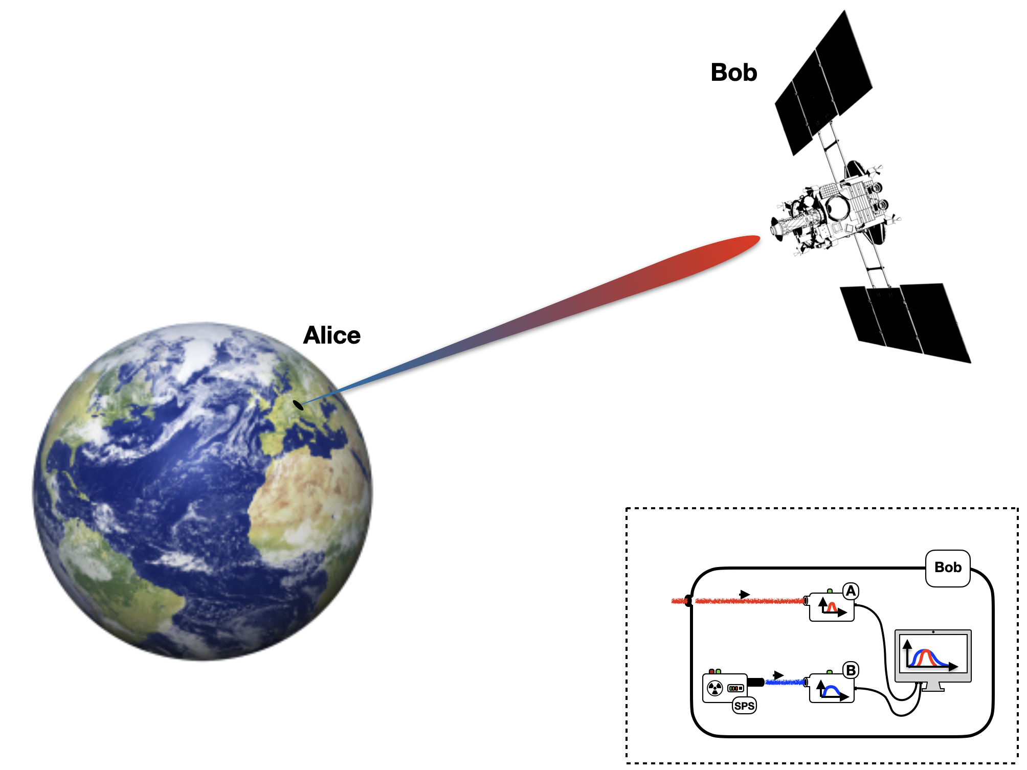
Alice and Bob wish to determine how gravitational redshift affects photons. Alice sends a photon to Bob, who will detect a gravitational redshift within the incoming photon, i.e., each sharp frequency $\omega^{\prime}$ as measured locally by his clock will not coincide with the sharp frequency $\omega$ of the sent photon. The scheme is depicted in Figure 1. As far as Bob is concerned, i.e., from the perspective of his laboratory, the expected photon has changed and he can study the properties of the transformation involved, irrespective of where the incoming photon has originated or which specific physical process it has undergone. Therefore, Bob can assign a channel to the process that affected the incoming photon, and seek for its properties.

Bob starts by assuming that there is a transformation $T(\chi):\omega\rightarrow\chi^{2}\omega$ on each sharp frequency $\omega$. He then looks for a unitary transformation $\hat{U}(\chi)$ that implements $T(\chi)$ through

for all $\chi$, where $\hat{U}^{\dagger}(\chi)\hat{U}(\chi)=\mathds{1}$.

Assuming that the transformation (4) holds, it is easy to use the explicit expression for $\hat{A}_{\omega_{0}}$, the fact that $[\hat{a}_{\chi^{2}\omega},\hat{a}_{\chi^{2}\omega^{\prime}}^{\dagger}]=\delta(\chi^{2}\omega-\chi^{2}\omega^{\prime})$, and $\delta(f(x))=\sum_{n}\delta(x-x_{0,n})/|f^{\prime}(x_{0,n})|$, where $x_{0,n}$ are the zeros of the function $f(x)$, to show that

This equation can be satisfied only when $\chi=1$, that is, for the trivial case of no redshift. Clearly, this cannot happen in general as can be seen from (3). Therefore, we conclude that gravitational redshift in the form of a linear shift of the spectrum of sharp frequencies cannot be obtained as the result of a unitary operation on the field modes $\{\hat{a}_{\omega}\}$ alone.²²2Note that if (4) were replaced by $\hat{a}_{\omega^{\prime}}=\hat{U}^{\dagger}(\chi)\,\hat{a}_{\omega}\,\hat{U}(\chi)=\chi\hat{a}_{\chi^{2}\omega}$, the commutation relations would be persevered. This result corroborates the claim that the gravitational redshift is not simply a shift in the sharp frequencies of the photons for all frequencies of the spectrum.

We now ask a more refined version of the question posed above: how is the transformation $T(\chi)$ implemented by a unitary operator when acting on realistic photons? To answer this question, we start by noting that Bob will describe the received photon as $\hat{A}_{\omega_{0}^{\prime}}=\int_{0}^{\infty}d\omega\,F^{\prime}_{\omega_{0}^{\prime}}(\omega/\sigma^{\prime})\,\hat{a}_{\omega}$ as a function of the local frequency $\omega$ as measured in his laboratory, while the expected photon has the expression $\hat{A}_{\omega_{0}}=\int_{0}^{\infty}d\omega\,F_{\omega_{0}}(\omega/\sigma)\,\hat{a}_{\omega}$. Bob then notices that each sharp frequency $\omega$ that appears in the definition of $\hat{A}_{\omega_{0}}$ transforms by $T(\chi):\omega\rightarrow\chi^{2}\omega$, see [10]. This means that

He can then identify the function $F^{\prime}_{\omega_{0}^{\prime}}(\omega/\sigma^{\prime})\equiv\chi\,F_{\omega_{0}}(\chi^{2}\omega/\sigma)=\chi\,F_{\omega_{0}/\chi^{2}}(\omega/(\sigma/\chi^{2}))$, where $\omega_{0}^{\prime}=\omega_{0}/\chi^{2}$ and $\sigma^{\prime}=\sigma/\chi^{2}$, which represents a well defined physical photon in the sense that $\int_{0}^{\infty}d\omega|F^{\prime}_{\omega_{0}^{\prime}}(\omega/\sigma^{\prime})|^{2}=1$. He is left with introducing the operator $\hat{a}_{\omega}^{\prime}:=\chi\hat{a}_{\chi^{2}\omega}$, which has well defined canonical commutation relations $[\hat{a}_{\omega}^{\prime},\hat{a}_{\omega}^{{\dagger}\prime}]=\delta(\omega-\omega^{\prime})$. We now note that the fact that $\hat{a}_{\omega}^{\prime},\hat{a}_{\omega}^{{\dagger}\prime}$ and $\hat{a}_{\omega},\hat{a}_{\omega}^{\dagger}$ have identical commutation relations for the same frequencies, and the fact that $\int d\omega\,\hbar\omega\,\hat{a}_{\omega}^{{\dagger}\prime}\hat{a}_{\omega}^{\prime}|1_{\omega}^{\prime}\rangle=\hbar\omega|1_{\omega}^{\prime}\rangle$, where $|1_{\omega}^{\prime}\rangle:=\hat{a}_{\omega}^{{\dagger}\prime}|0\rangle$, imply that Bob cannot distinguish locally between $\hat{a}_{\omega}$ and $\hat{a}_{\omega}^{\prime}$, and he therefore identifies $\hat{a}_{\omega}^{\prime}\equiv\hat{a}_{\omega}$. Bob therefore can assume that the following unitary transformation has occurred

with the relation $F^{\prime}_{\omega_{0}^{\prime}}(\omega/\sigma^{\prime})\equiv\chi F_{\omega_{0}}(\chi^{2}\omega/\sigma)$. Notice that the transformation (7) applies appropriately to all of the photon operators $\{\hat{A}_{\omega_{0}},\hat{A}_{\underline{\lambda}}\}$ and implies, equivalently, that there is a canonical transformation of the bases $\{F_{\omega_{0}},F_{\underline{\lambda}}\}$ and $\{F^{\prime}_{\omega_{0}^{\prime}},F^{\prime}_{\underline{\lambda}^{\prime}}\}$ of mode functions.

We can collect all field operators $\{\hat{A}_{\omega_{0}},\hat{A}_{\underline{\lambda}}\}$ in the vector $\hat{\mathbb{X}}:=(\hat{A}_{\omega_{0}},\hat{A}_{\underline{\lambda}_{1}},\ldots)^{\textrm{Tp}}$. Then, the transformation (7) implies that there exists a unitary matrix $\boldsymbol{U}(\chi)$ such that

This transformation is known in quantum optics as a mode-mixer [28], and it is a particular case of a symplectic transformation [29]. Note that, if we choose $N$ modes to study, there are $N(N+1)$ independent overlaps of the form $\langle F_{n},F_{m}\rangle$ (including the modulus and the phase). The overlaps with $F_{\perp}$ are uniquely fixed this way as well. A transformation of the form (8), on the other hand, is determined by the $(N+1)\times(N+1)$ unitary matrix $\boldsymbol{U}(\chi)$ that mixes the $N$ chosen modes with the orthogonal complement $F_{\perp}$. Therefore, the independent angles that define $\boldsymbol{U}(\chi)$ are $(N+1)N/2$, and there are also $(N+1)N/2$ independent phases. Since the degrees of freedom match in number, it is a well posed operation to identify the angles of $\boldsymbol{U}(\chi)$ through the independent overlaps $|\langle F_{n},F_{m}\rangle|$, and the phases of $\boldsymbol{U}(\chi)$ with $\textrm{arg}(\langle F_{n},F_{m}\rangle)$, as also noted in the literature [30].

Let us focus on the case where we select two different commuting photon operators $\hat{A}_{\omega_{0}}$ and $\hat{A}_{\tilde{\omega}_{0}}$, and let us consider the transformed modes $\hat{A}_{\omega_{0}^{\prime}}$ and $\hat{A}_{\tilde{\omega}_{0}^{\prime}}$. We then define the vector $\hat{\mathbb{X}}:=(\hat{A}_{\omega_{0}},\hat{A}_{\tilde{\omega}_{0}},\hat{A}_{\perp})^{\textrm{Tp}}$, where the operator $\hat{A}_{\perp}:=\sum_{\underline{\lambda}}\alpha_{\underline{\lambda}}\,\hat{A}_{\underline{\lambda}}$ collects all of the operators orthogonal to the two chosen ones, we have $\sum_{\underline{\lambda}}|\alpha_{\underline{\lambda}}|^{2}=1$, and $\hat{A}_{\perp^{\prime}}:=\hat{U}^{\dagger}(\chi)\,\hat{A}_{\perp}\,\hat{U}(\chi)$. The general transformation (8) is therefore defined by the symplectic representation of the product of three beam-splitting operations of the form $\exp[\theta(e^{i\varphi_{\theta}}\hat{A}_{\omega_{0}}\hat{A}_{\perp}^{\dagger}-e^{-i\varphi_{\theta}}\hat{A}_{\omega_{0}}^{\dagger}\hat{A}_{\perp})]$, $\exp[\psi(e^{i\varphi_{\psi}}\hat{A}_{\tilde{\omega}_{0}}\hat{A}_{\perp}^{\dagger}-e^{-i\varphi_{\psi}}\hat{A}_{\tilde{\omega}_{0}}^{\dagger}\hat{A}_{\perp})]$ and $\exp[\phi(e^{i\varphi_{\phi}}\hat{A}_{\omega_{0}}\hat{A}_{\tilde{\omega}_{0}}^{\dagger}-e^{-i\varphi_{\phi}}\hat{A}_{\omega_{0}}^{\dagger}\hat{A}_{\tilde{\omega}_{0}})]$. We report the explicit result for $\varphi_{\theta}=\varphi_{\phi}=\varphi_{\psi}=0$, and note that the phases can be restored when necessary. We have

where we introduce $\textrm{s}_{\vartheta}:=\sin\vartheta$ and $\textrm{c}_{\vartheta}:=\cos\vartheta$ for ease of presentation. The transformation (9) is known in quantum optics as a three-wave mode-mixer, or tritter [28, 30].

Most importantly, the angles $\theta$, $\phi$ and $\psi$ are functions of the redshift $\chi$ and are defined through

We expect that $\theta$, $\phi$ and $\psi$, in the redshift regime $\chi\geq 1$, take values between $\theta=\phi=\psi=0$ (i.e., perfect overlap), and $\theta=\psi=\pi/2$, $\phi=0$ (complete mismatch). An analogous analysis can be done for the blueshift regime $0\leq\chi<1$.

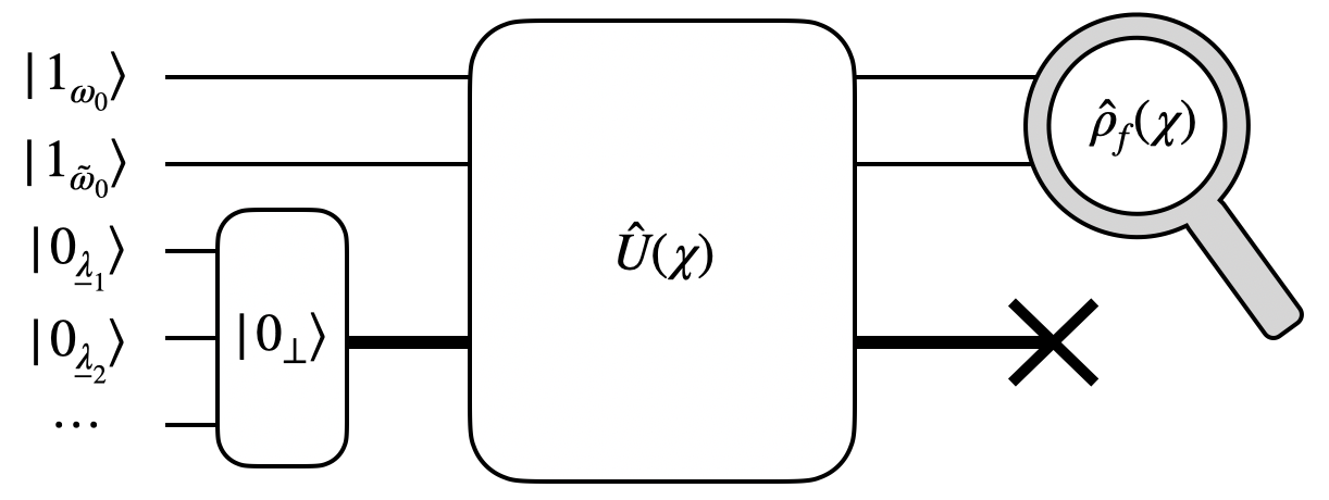
Here we describe a photon-exchange task between Alice and Bob that exploits the transformation (9) to show that gravity induces quantum interference of photonic states. It is depicted using a circuit implementation language in Figure 2.

The steps required to perform the task read as follows:

• i.

  Alice prepares a two-photon separable state $|\Psi_{0}\rangle:=|1_{\omega_{0}}1_{\tilde{\omega}_{0}}0\rangle$ and sends it to Bob, who receives it as $|\Psi\rangle:=|1_{\omega_{0}^{\prime}}1_{\tilde{\omega}_{0}^{\prime}}0\rangle$. Introducing the notation $|nmp\rangle:=\frac{(\hat{A}^{{\dagger}}_{\omega_{0}})^{n}}{\sqrt{n!}}\frac{(\hat{A}^{{\dagger}}_{\tilde{\omega}_{0}})^{m}}{\sqrt{m!}}\frac{(\hat{A}^{{\dagger}}_{\perp})^{p}}{\sqrt{p!}}|0\rangle$, it is immediate to verify that Bob’s state reads locally as

  	$\displaystyle|\Psi\rangle=$	$\displaystyle\sqrt{2}\left[U_{13}U_{23}|002\rangle+U_{12}U_{22}|020\rangle+U_{11}U_{21}|200\rangle\right]$
  	$\displaystyle+$	$\displaystyle(U_{13}U_{22}+U_{12}U_{23})|011\rangle+(U_{11}U_{22}+U_{12}U_{21})|110\rangle$
  	$\displaystyle+$	$\displaystyle(U_{11}U_{23}+U_{13}U_{21})|101\rangle.$		(11)

  Here $U_{ab}$ are the coefficients of the matrix (9).

• ii.

  The final state $\hat{\rho}_{\textrm{f}}(\chi)$ of the modes $\hat{A}_{\omega_{0}}$ and $\hat{A}_{\tilde{\omega}_{0}}$ in Bob’s laboratory is obtained by tracing (i.) over the unovserbed subsystem degrees of freedom $\hat{A}_{\perp}$, and it is easy to compute but gives a cumbersome expression. We give its generic form here

  	$\displaystyle\hat{\rho}_{\textrm{f}}(\chi)=$	$\displaystyle\rho_{0000}|00\rangle\langle 00|+\rho_{0202}|02\rangle\langle 02|+\rho_{2020}|20\rangle\langle 20|$
  	$\displaystyle+$	$\displaystyle\rho_{1010}|10\rangle\langle 10|+\rho_{0101}|01\rangle\langle 01|+\rho_{1111}|11\rangle\langle 11|$
  	$\displaystyle+$	$\displaystyle\rho_{2011}|20\rangle\langle 11|+\rho_{0211}|02\rangle\langle 11|$
  	$\displaystyle+$	$\displaystyle\rho_{2001}|20\rangle\langle 02|+\rho_{1001}|10\rangle\langle 01|+\textrm{h.c.}$		(12)

  The coefficients $\rho_{nmpq}$ can be obtained in terms of the matrix elements $U_{ab}$ with simple algebra. We avoid printing them here to improve clarity of presentation.

We note here that it is possible to have all terms in (ii.) that include a $|11\rangle$ contribution to vanish with either $\rho_{0202}$ or $\rho_{2020}$ remaining nonzero. It is sufficient that either $U_{11}=U_{21}=0$ while $U_{12},U_{22}$ are both nonzero, or viceversa. In the first case we obtain the fully mixed state $\hat{\rho}_{\textrm{f}}(\chi)=2|U_{13}U_{23}|^{2}|00\rangle\langle 00|+2|U_{12}U_{22}|^{2}|02\rangle\langle 02|+|U_{13}U_{22}+U_{12}U_{23}|^{2}|01\rangle\langle 01|$. The other case can be obtained in a similar fashion.

More importantly, however, is the case when $\rho_{1111}=0$, but $\rho_{0202}\neq 0$ and $\rho_{2020}\neq 0$ at the same time. This requires us to assume that $|U_{11}U_{22}+U_{12}U_{21}|=|c_{\theta}(c_{\phi}^{2}-s_{\phi}^{2})c_{\psi}-s_{\theta}s_{\phi}s_{\psi}|=0$, which can occur given the freedom in choice of the initial modes. In this case, all terms in (ii.) with $|11\rangle$ vanish, and we are left with a state that exhibits Hong-Ou-Mandel-like interference [31, 32]. This is a genuine quantum effect due to gravity.

We can finally verify if the state (ii.) is entangled. This requires the partial transpose $\hat{\rho}^{\textrm{pt}}_{\textrm{f}}(\chi)$ (with respect, say, of the second mode) of the state, and the use of the negativity $\mathcal{N}(\hat{\rho}_{\textrm{f}}(\chi)):=\max\{0,1/2\sum_{\lambda<0}(|\lambda|-\lambda)\}$, where $\lambda$ are the eigenvalues of $\hat{\rho}^{\textrm{pt}}_{\textrm{f}}(\chi)$. If the negativity is nonzero, the PPT criterion guarantees that the state is entangled [33]. We can only find explicitly two negative eigenvalues of the partial transpose, which are sufficient for the detection. In fact, some algebra gives us

which is greater than $0$ for values at least one of $\rho_{0211}$ or $\rho_{2011}$ greater than zero. When this occurs, we conclude that gravitational redshift has entangled the state. Note that in the case where $\rho_{1111}=0$ we also have $\rho_{0211}=\rho_{2011}=0$, which implies that the right-hand side of (IV.2) also vanishes. In this case, in order to detect entanglement we need to compute the other negative eigenvalues either analytically of numerically. This poses no conceptual difficulty, and can be therefore done when required.

References

- Misner et al. [1973] C. W. Misner, K. S. Thorne, and J. A. Wheeler, San Francisco: W.H. Freeman and Co., 1973, edited by Misner, C. W., Thorne, K. S., & Wheeler, J. A. (1973).
- Wilhelm and Dwivedi [2014] K. Wilhelm and B. N. Dwivedi, New Astronomy 31, 8 (2014).
- Pound and Rebka [1959] R. V. Pound and G. A. Rebka, Phys. Rev. Lett. 3, 439 (1959).
- Müller, A. and Wold, M. [2006] Müller, A. and Wold, M., A&A 457, 485 (2006).
- Chou et al. [2010] C. W. Chou, D. B. Hume, T. Rosenband, and D. J. Wineland, Science 329, 1630 (2010).
- Müller et al. [2010] H. Müller, A. Peters, and S. Chu, Nature 463, 926 (2010).
- Will [2014] C. M. Will, Living Reviews in Relativity 17, 4 (2014).
- Litvinov et al. [2018] D. Litvinov, V. Rudenko, A. Alakoz, U. Bach, N. Bartel, A. Belonenko, K. Belousov, M. Bietenholz, A. Biriukov, R. Carman, et al., Physics Letters A 382, 2192 (2018).
- Di Pumpo et al. [2021] F. Di Pumpo, C. Ufrecht, A. Friedrich, E. Giese, W. P. Schleich, and W. G. Unruh, PRX Quantum 2, 040333 (2021).
- Bruschi et al. [2014a] D. E. Bruschi, T. C. Ralph, I. Fuentes, T. Jennewein, and M. Razavi, Phys. Rev. D 90, 045041 (2014a).
- Bruschi et al. [2014b] D. E. Bruschi, A. Datta, R. Ursin, T. C. Ralph, and I. Fuentes, Phys. Rev. D 90, 124001 (2014b).
- Kohlrus et al. [2017] J. Kohlrus, D. E. Bruschi, J. Louko, and I. Fuentes, EPJ Quantum Technology 4, 7 (2017).
- Nielsen and Chuang [2010] M. A. Nielsen and I. L. Chuang, Quantum Computation and Quantum Information: 10th Anniversary Edition (Cambridge University Press, 2010).
- Bassi et al. [2017] A. Bassi, A. Großardt, and H. Ulbricht, Classical and Quantum Gravity 34, 193002 (2017).
- Howl et al. [2019] R. Howl, R. Penrose, and I. Fuentes, New Journal of Physics 21, 043047 (2019).
- Carney et al. [2019] D. Carney, P. C. E. Stamp, and J. M. Taylor, Classical and Quantum Gravity 36, 034001 (2019).
- Williams et al. [2016] J. Williams, S. wey Chiow, N. Yu, and H. Müller, New Journal of Physics 18, 025018 (2016).
- Tino [2021] G. M. Tino, Quantum Science and Technology 6, 024014 (2021).
- Smith and Ahmadi [2019] A. R. H. Smith and M. Ahmadi, Quantum 3, 160 (2019).
- Smith and Ahmadi [2020] A. R. H. Smith and M. Ahmadi, Nature Communications 11, 5360 (2020).
- Bruschi and Wilhelm [2020] D. E. Bruschi and F. K. Wilhelm, arXiv:2006.11768 [quant-ph] (2020).
- Birrell and Davies [1982] N. D. Birrell and P. C. W. Davies, Quantum Fields in Curved Space, Cambridge Monographs on Mathematical Physics (Cambridge University Press, 1982).
- Srednicki [2007] M. Srednicki, Quantum Field Theory (Cambridge University Press, 2007).
- Exirifard et al. [2021] Q. Exirifard, E. Culf, and E. Karimi, Communications Physics 4, 10.1038/s42005-021-00671-8 (2021).
- Exirifard and Karimi [2022] Q. Exirifard and E. Karimi, Physical Review D 105, 10.1103/physrevd.105.084016 (2022).
- Okun [2000] L. B. Okun, Modern Physics Letters A 15, 1941 (2000).
- Wald [1984] R. M. Wald, General relativity (Chicago Univ. Press, Chicago, IL, 1984).
- Scully and Zubairy [1997] M. O. Scully and M. S. Zubairy, Quantum Optics (Cambridge University Press, 1997).
- Adesso et al. [2014] G. Adesso, S. Ragy, and A. R. Lee, Open Syst. Inf. Dyn. 21, 1440001 (2014).
- Menssen et al. [2017] A. J. Menssen, A. E. Jones, B. J. Metcalf, M. C. Tichy, S. Barz, W. S. Kolthammer, and I. A. Walmsley, Phys. Rev. Lett. 118, 153603 (2017).
- Hong et al. [1987] C. K. Hong, Z. Y. Ou, and L. Mandel, Phys. Rev. Lett. 59, 2044 (1987).
- Bouchard et al. [2020] F. Bouchard, A. Sit, Y. Zhang, R. Fickler, F. M. Miatto, Y. Yao, F. Sciarrino, and E. Karimi, Reports on Progress in Physics 84, 012402 (2020).
- Peres [1996] A. Peres, Phys. Rev. Lett. 77, 1413 (1996).
- Bruschi et al. [2021] D. E. Bruschi, S. Chatzinotas, F. K. Wilhelm, and A. W. Schell, Physical Review D 104, 10.1103/physrevd.104.085015 (2021).
- Carroll [2019] S. M. Carroll, Spacetime and Geometry: An Introduction to General Relativity (Cambridge University Press, 2019).
- Oi et al. [2017] D. K. Oi, A. Ling, G. Vallone, P. Villoresi, S. Greenland, E. Kerr, M. Macdonald, H. Weinfurter, H. Kuiper, E. Charbon, and et al., EPJ Quantum Technology 4 (2017).
- Joshi et al. [2018] S. K. Joshi, J. Pienaar, T. C. Ralph, L. Cacciapuoti, W. McCutcheon, J. Rarity, D. Giggenbach, J. G. Lim, V. Makarov, I. Fuentes, T. Scheidl, E. Beckert, M. Bourennane, D. E. Bruschi, A. Cabello, J. Capmany, A. Carrasco-Casado, E. Diamanti, M. Dušek, D. Elser, A. Gulinatti, R. H. Hadfield, T. Jennewein, R. Kaltenbaek, M. A. Krainak, H.-K. Lo, C. Marquardt, G. Milburn, M. Peev, A. Poppe, V. Pruneri, R. Renner, C. Salomon, J. Skaar, N. Solomos, M. Stipčević, J. P. Torres, M. Toyoshima, P. Villoresi, I. Walmsley, G. Weihs, H. Weinfurter, A. Zeilinger, M. Żukowski, and R. U. and, New Journal of Physics 20, 063016 (2018).
- Mazzarella et al. [2020] L. Mazzarella, C. Lowe, D. Lowndes, S. K. Joshi, S. Greenland, D. McNeil, C. Mercury, M. Macdonald, J. Rarity, and D. K. L. Oi, Cryptography 4, 10.3390/cryptography4010007 (2020).
- Belenchia et al. [2022] A. Belenchia, M. Carlesso, Ömer Bayraktar, D. Dequal, I. Derkach, G. Gasbarri, W. Herr, Y. L. Li, M. Rademacher, J. Sidhu, D. K. Oi, S. T. Seidel, R. Kaltenbaek, C. Marquardt, H. Ulbricht, V. C. Usenko, L. Wörner, A. Xuereb, M. Paternostro, and A. Bassi, Physics Reports 951, 1 (2022).
- Altschul et al. [2015] B. Altschul, Q. G. Bailey, L. Blanchet, K. Bongs, P. Bouyer, L. Cacciapuoti, S. Capozziello, N. Gaaloul, D. Giulini, J. Hartwig, L. Iess, P. Jetzer, A. Landragin, E. Rasel, S. Reynaud, S. Schiller, C. Schubert, F. Sorrentino, U. Sterr, J. D. Tasson, G. M. Tino, P. Tuckey, and P. Wolf, Advances in Space Research 55, 501 (2015).
- Tino et al. [2020] G. Tino, L. Cacciapuoti, S. Capozziello, G. Lambiase, and F. Sorrentino, Progress in Particle and Nuclear Physics 112, 103772 (2020).
- Bassi et al. [2022] A. Bassi, L. Cacciapuoti, S. Capozziello, S. Dell’Agnello, E. Diamanti, D. Giulini, L. Iess, P. Jetzer, S. K. Joshi, A. Landragin, C. L. Poncin-Lafitte, E. Rasel, A. Roura, C. Salomon, and H. Ulbricht, npj Microgravity 8, 49 (2022).
- Zych and Brukner [2018] M. Zych and Č. Brukner, Nature Physics 14, 1027 (2018).
- Barzel et al. [2022] R. Barzel, D. E. Bruschi, A. W. Schell, and C. Lämmerzahl, Physical Review D 105, 10.1103/physrevd.105.105016 (2022).
- Bellini et al. [2014] G. Bellini, L. Ludhova, G. Ranucci, and F. L. Villante, Advances in High Energy Physics 2014, 1 (2014), publisher: Hindawi Limited.
- Salas et al. [2021] P. F. d. Salas, D. V. Forero, S. Gariazzo, P. Martínez-Miravé, O. Mena, C. A. Ternes, M. Tórtola, and J. W. F. Valle, Journal of High Energy Physics 2021, 10.1007/jhep02(2021)071 (2021), publisher: Springer Science and Business Media LLC.
- Chang [2018] D. C. Chang, Optik 174, 636 (2018).