Gravitational waves excited by binary stars orbiting around a supermassive black hole
Abstract
Binary stars are as frequency as single stars in the Universe, and at least 70% of the massive stars located in our Galaxy belong to a binary system. We produce the gravitational waveforms for the extreme mass ratio inspiral systems (EMRIs) of binary stars moving around central supermassive black hole (SBH), or called B-EMRIs.We calculate the orbits of such systems via the Hamilton-Jacobi approach. To improve accuracy we adopt the quadrupole-octupole expression of gravitational wave (GW) and study the contribution of radiation reaction. Compared to the waveforms of EMRIs, there are higher frequency oscillations superposed on the waveforms of B-EMRIs. We perform frequency spectrum analysis of the GW waveforms, and find that higher frequency signals give their prominency in the waveforms of B-EMRIs. We study the binary compact objects with different masses and inclination angles of the binary internal orbit plane, and obtain the frequency spectrum variation with respect to the parameters. To obtain more precise result for future observation of GWs from space-based detector, we take into account gravito-electromagnetic (GEM) force for the binary orbit on the equatorial plane, and compare the waveforms with that of EMRIs without GEM force. The result of mismatch shows that the waveforms of B-EMRIs are credibly distinguishable by the space-based GW detectors when GEM force is considered.
1 Introduction
Black hole (BH) may be the most thoroughly-studied object before its discovery in the history of science. Recently, the Event Horizon Telescope (EHT) collaboration announced the images of the SBHs M87* and SgrA*[1, 2]. Such images together with the detections of GWs[3, 4] confirm the existence of black holes, and launch a new era of testing gravity in strong-field regime and far beyond the scale of solar system.
The goal of next generation space-based GW detectors—Taiji, Tianqin, and Laser Interferometer Space Antenna (LISA)—is designed to be most sensitive to detect low frequency GW signals in the band about Hz. EMRIs are the sources generating GWs in this band. EMRIs are composed of central SBH and stellar-mass compact objects moving around the SBH. The multi-body interaction in the cusp of the stellar population surrounding the SBH may scatter the compact objects into the orbits close the central SBH and form the EMRIs[5, 6]. The GWs generated by EMRIs carry the information both of the background BH and the stellar-mass compact objects, so detections of GWs will help to learn more about the the strong-field character of the BH spacetime, the multipole structure of the BH, the structures of the small body compact objects, and the information of the underlying theory governing the way in which our universe works.
Analysis of the data released by GW detectors replies heavily on the matched filtering technique, which makes correlations between data and template waveforms, thus establishing template waveforms of EMRIs is critical for data analysis.
The waveforms generated by motions of single stellar-mass compact object in BH spacetime have been studied intensively[7, 8, 9, 10, 11, 12, 13, 14, 15, 16, 17, 18, 19, 20, 21, 22, 23, 24], including probe of fundamental fields[25, 26], modified gravity[27, 28, 29, 30, 31, 32], extra dimensions[33], electric charge and internal structure of small body objects[34, 36, 35, 37, 38, 39, 40], etc. Binary-star systems are important astrophysical objects which are constituted of binary stars revolving around each other. The amount of binary-star systems is huge in the Galaxy. It’s estimated that the amount of binary-star systems is no less than that of single star. The vast majority of stars are located in a binary system. It is estimated that more than 70% of all massive stars may exist in systems with two or three stars.
In active galactic nuclei, due to the rich forms of interactions between SBH, the gaseous accretion disks and the stellar mass compact objects, the binary may be formed and scattered onto the orbits closed to the central SBH to form the systems which we call B-EMRIs. The binary stars orbiting around central SBH constitute a significant typical EMIRs. Thus, it is quite sensible to consider the waveforms produced by motions of binary stars surrounding a SBH in addition to the case of single star. The GW generated by each of the binary star overlaps, so the waveforms generated by this type of EMRIs are distinguishable from that generated by single star. In this paper, we consider the case that the amplitudes of the GW generated by internal motion of binary stars are small compared to that generated by external motion of the mass center since such systems are considerable popular in the Universe and can be detected by the next generation observatory of GWs. It’s expected small perturbations would appear in B-EMRIs when compared to the waveforms of ordinary EMRIs. It’s really worthwhile to build the template waveforms of such systems for future data analysis of space-based detectors for GWs.
Since the traditional method of calculating gravitational waveforms—solving Teukolsky equations—cost a lot of time and computational resources[41, 42, 43, 44, 45, 46, 47, 48, 49, 50, 51, 52, 53], while realistic data analysis need to handle a large number of waveforms, thus more practical methods are necessary. And it is proved that such methods are feasible. In this paper, we adopt the “numerical kludge” (NK) method which generates waveforms more conveniently and quickly but captures the principle feature of true waveforms[54]. To improve accuracy, aside from the mass quadrupole we take into account the mass octupole and current quadrupole moments of the source to solve the wave equations. It’s justified the NK method does excellently at approximating the true gravitational waveforms so this method has already been used for scoping out data analysis of LISA. For the radiation reaction, we consider the adiabatic evolution of orbit parameters: the timescale of evolution of the orbit parameters is much larger than that of orbit cycles such that the motion of mass point in BH spacetime is nearly geodesic. Further, since the amplitude of GWs generated by internal motions are smaller compared to that generated by external motions of the mass center, to master the principle property of the waveform we concentrate on the radiation reaction due to the GW emissions generated by the motion of mass center. We take the hybrid scheme that combines Tagoshi’s[46], Shibata’s[53] and Ryan’s fluxes[55, 56], whose precision is comparable or higher than Teukolsky-based results for generic circular-inclined orbits [57].
According to equivalence principle only at the origin of free-fall frame (FFF), i.e., the mass center of the binary, the spacetime is flat, if there is departure from the origin the effects of curved spacetime appear. Since for binary system, either star does not locate at the origin of FFF, we should take into account the gravitational effects caused by this reason. Later we’ll study the effects of GEM force on the waveforms of B-EMRIs.
The paper is organised as follows. In section 2 we calculate the trajectories of the binary stars and give waveforms of GW with the NK method. In section 3 we analyse the waveforms by calculating mismatch between the waveforms of binary stars and that of single star. We summarize our results in the last section. In this work, we adopt the geometrized units with .
2 Numerical Kludge Waveforms
In this section we adopt the NK waveforms approach developed in [54] to produce the GW waveforms of the B-EMRIs. We consider the system as, the central SBH is Kerr, the stellar-mass binary stars revolve around each other and they as a whole move along the inspiral trajectory of the central SBH. The binary stars are supposed to live far away from the SBH such that the internal gravity between them dominates, so the impacts of the SBH on the internal orbit of the binary stars are neglected, while the center of mass of the binary stars is still on the inspiral trajectory of the SBH. The geometry of binary stars moving in the spacetime of SBH is illustrated in Fig.1.
2.1 the geometry of the orbit
The binary are supposed to revolve around each other along elliptic orbit. We introduce the relative coordinates , with , then the coordinates of the binary with masses and can be expressed with coordinates of mass center and relative coordinates as , where . We use the coordinates and parameters with tilde to describe the internal motion of binary stars around each other. The spin axis of the central SBH is along , as displayed in Fig.1, is the angle between and which is the normal direction of the surface of binary stars’ internal elliptic orbit. is the angle between and the node line which is the intersection line between the surface of binary stars’ internal orbit and the horizonal surface.
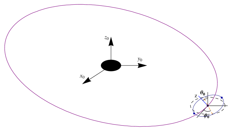
.
Now let’s discuss the orbit of a mass point in Kerr spacetime, in Boyer-Lindquist coordinates Kerr metric can be expressed as
| (1) |
where and . We adopt the Hamilton-Jacobi formulation, the Hamilton-Jacobi equation reads
| (2) |
The Kerr BH admits two obvious Killing vectors and , which correspond to two conserved charges, energy and angular momentum , so for the mass point with mass ( in this paper), the action reads
| (3) |
which leads to and . Inserting (3) into the Hamilton-Jacobi equation (2) and separating variables we have
| (4) |
with
| (5) | ||||
where is a constant which is related with the separation constant through . Actually, the variable-separability of Hamilton-Jacobi equation in Kerr spacetime corresponds to a nontrivial symmetry which is described by a Killing tensor
| (6) |
The Killing tensor satisfies the Killing equation , the bracket denotes symmetrization of the indices. This is a highly nontrivial symmetry which corresponds to the third conserved quantity—Carter constant —in addition to energy and angular momentum[58]. The explicit integration expression of coordinates can be obtained by setting the partial derivative of Hamilton-Jacobi function with respect to the constants of motion to be zero, that’s to say the motions of particles in Kerr spacetime are integrable.


With the above results, one now is able to give the geodesics of a mass point in Kerr spacetime
| (7) | ||||
with
| (8) | ||||
To solve the equations of geodesic motions (7) numerically, we introduce two angular variables and in place of and to avoid possible singularities. is defined as
| (9) |
It’s evident the periastron and apastron locate at and . is defined as , where is given by
| (10) |
with . The parameter ranges from 0 to . As varies from 0 to , goes from one turning point to the other and back to . We introduce an “inclination angle” to replace Carter constant . For or , equals to zero, from the geodesic equations (7) and (8) we know mass points remain on the equatorial plane at all times in this case. So corresponds to the equatorial orbits while corresponds to non-equatorial orbits. Expanding the radial potential as
| (11) |
we find evolution equations for and to be of the form
| (12) | ||||
where . Solving these equations allow us to know the positions of mass center of the binary at any time.
To calculate GWs, we need to calculate the positions of the two compact objects in binary system relative to the mass center. The mass center of the binary system is free-falling around the SBH, thus locally the spacetime around the mass center can be treated as Minkowskian spacetime. Since for binary system the size of their internal orbit is much smaller than that of their external orbit, i.e., is much smaller than , so the internal motions of binary are dominated by internal Newtonian gravity. For convenience, the two-body problem is reduced to one-body problem, the relative motion is described by the Lagrangian
| (13) |
where is the reduced mass, and the potential describes the internal gravity.
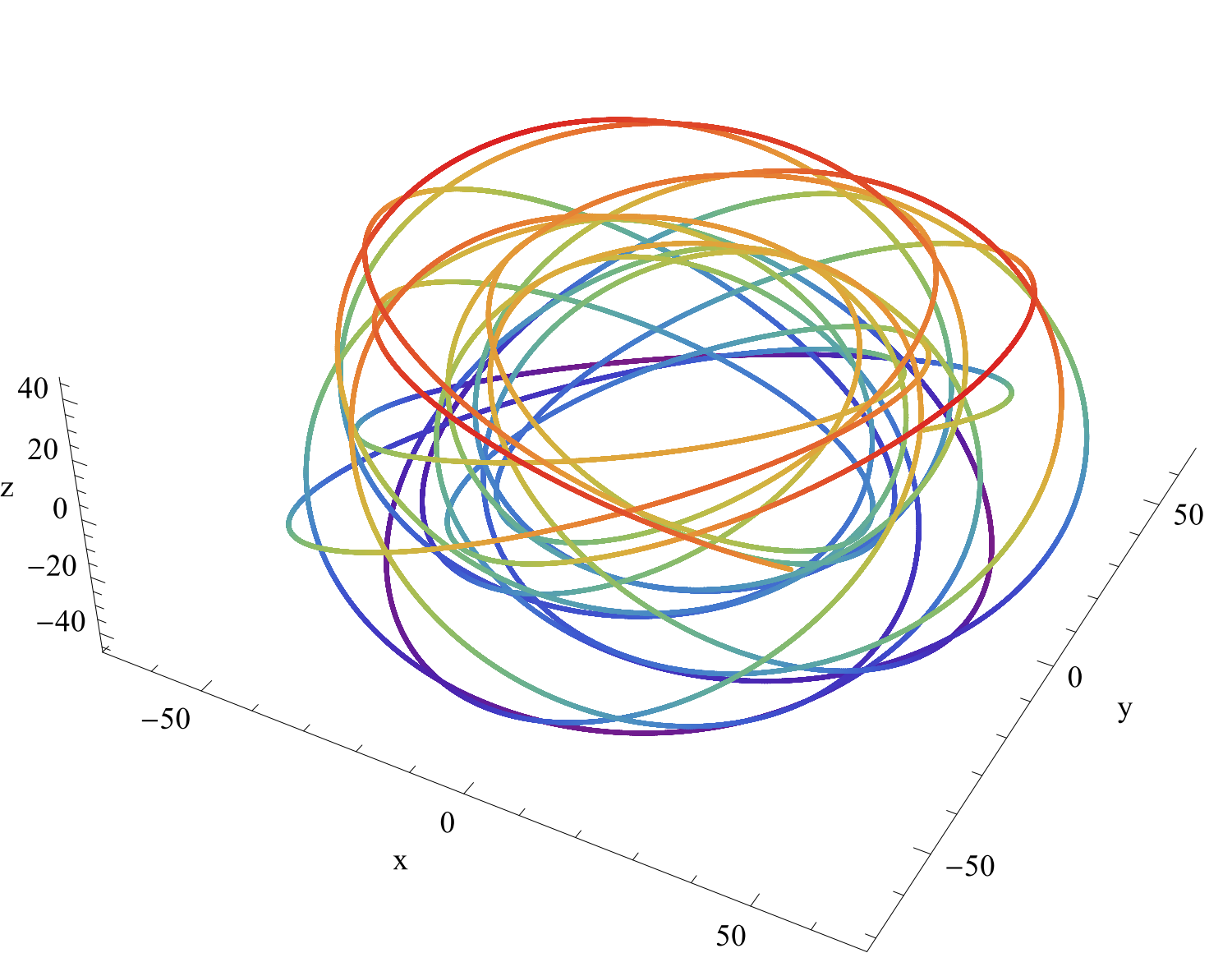
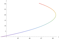
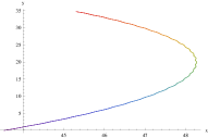
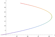
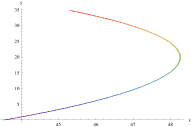
Solving the aforementioned equations that determine the motions of mass center and the internal motions allow us to give the orbit of the binary. In Fig.2 we show the orbits of one of the compact objects in the binary system. From the lower three detail images in Fig.2 one sees that, due to internal motions the orbit have small fluctuations, and thus the orbits fluctuate more frequently as mass increases. The reason roots in that if keeping other parameters fixed, the cycle of orbit becomes shorter as the mass of gravitational source increases. The fluctuations are expected to give rise to higher-frequency GWs.
2.2 the GW waveform
In the weak-field situation, the metric can be decomposed as , where is the flat metric and is small perturbation. By introducing the traceless tensor with , then the Einstein equations can be recast to the form
| (14) |
Here denotes the energy-momentum tensor of the source. In the slow motion limit, the GW is given by the quadrupole-octupole formula
| (15) |
with
| (16) | ||||
being the mass quadrupole moment, current quadrupole moment and mass octupole moment respectively, and , , where is the location of the observer.
In the NK prescription, a flat-space trajectory which is “equivalent” to a geodesic in Kerr spacetime is reconstructed by projecting the Boyer-Lindquist coordinates onto a fictitious spherical polar grid. A particle moving along geodesic path in Kerr spacetime can be viewed as the particle moving along curved path in flat-space, so it’s convenient for us to calculate GWs with Cartesian coordinates. In Cartesian coordinates the positions of one of the compact objects is given by
| (17) | ||||
where is the angle between the line connecting mass center and one of the compact objects and the line that lies in the plane of binary internal orbit and is perpendicular to the node line. For the position of the other compact object one only has to replace with in the above expression.
The expression (15) are valid for a general extended source in flat-space. For a single mass point with mass the energy-momentum tensor in flat spacetime is given by
| (18) |
For binary stars we know the energy-momentum tensor is the sum of two such terms with and respectively. The momenta (16) now can be simplified to
| (19) | ||||
Substituting (19) into (15) one then obtains the GW generated by a mass point. For binary system the GW is the superposition of that generated by two compact objects.
In the standard transverse-traceless (TT) gauge, the waveform is given by the TT projection of (15). The orthonormal basis of spherical coordinates is defined as
| (20) |
where the angles denote the observation point’s latitude and azimuth respectively. After TT projection the waveform is given by
| (21) |
with
| (22) | ||||
The usual “plus” and “cross” waveform polarizations are given by and respectively.
Due to the GW emissions, the compact objects will lose energy and angular momentum, although the amount of energy and angular momentum carried away by GWs is very small, the trajectory will alter accordingly, for a more precise study we consider backreaction of energy loss to the orbit. We study generic inclined-eccentric orbits of the center of mass of binary stars rather than just orbits on the equatorial plane. As we will see, since the amplitude of GW generated by internal motions of binary stars is small compared to that generated by external motions, we only consider the radiation reaction caused by the external motion of binary stars around the SBH while that caused by the internal motion is neglected. We consider the flux of generic orbits to 2nd order post-Newtonian approximation[57]
| (23) | ||||
where . The angle shows the inclination of internal orbit with respect to the external orbit through the Carter constant,
| (24) |
We defer the expressions of the coefficients to the Appendix. This expression of fluxes are the results of combining Tagoshi’s[46], Shibata’s [53] and Ryan’s fluxes [55, 56]. Numerical analysis indicates that these results ameliorate the unphysical inspiral properties for nearly circular and polar orbits, such as the inspiral moves rapidly away from circularity for the trajectories near zero eccentricity , and there is discontinuity between trajectories with slightly less than and those slightly above , etc., thus the fluxes (23) produce more physical reasonable results than previous ones. From the fluxes (23), we obtain the evolution of eccentricity and semi-latus rectum
| (25) | ||||
we obtain
| (26) | ||||
where we have
| (27) | ||||
Using the relation between inclination angle and Carter constant , one has
| (28) |


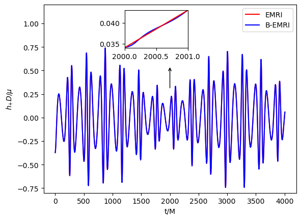
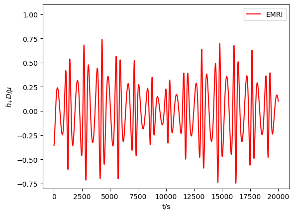
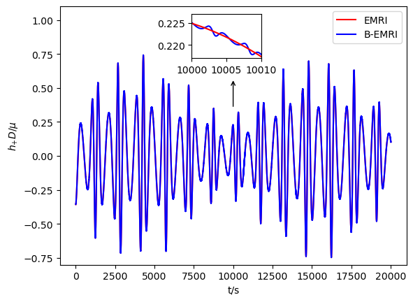
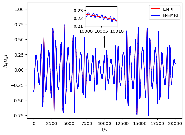
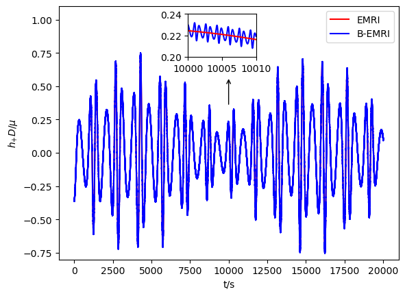
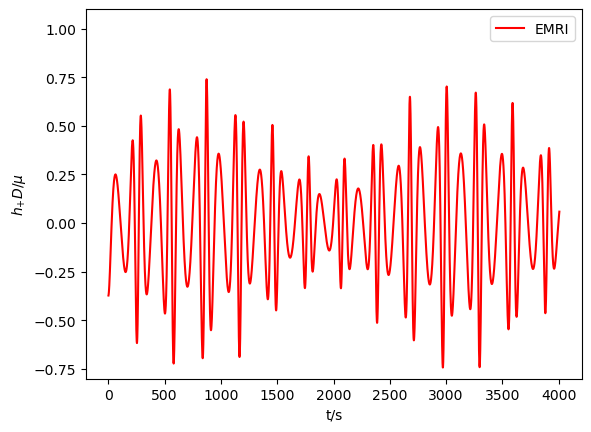
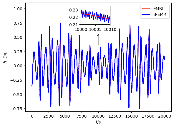
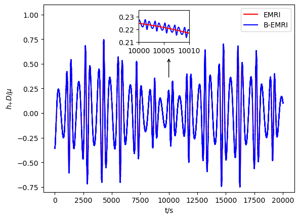
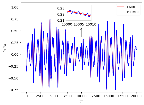
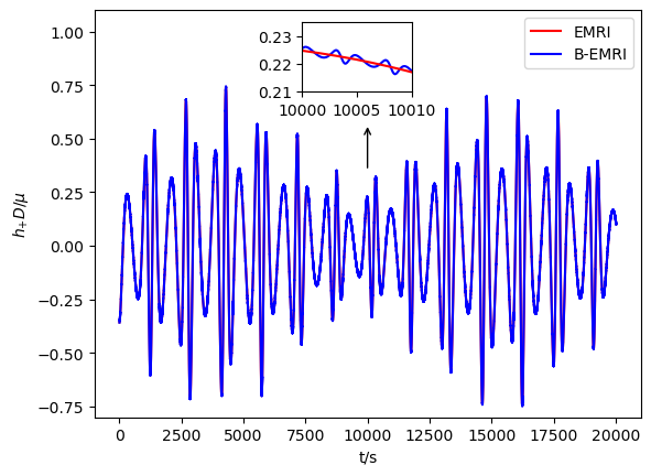
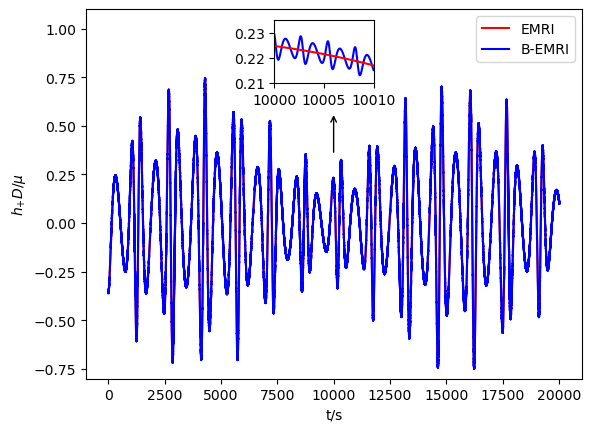
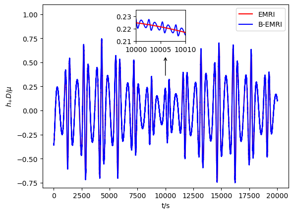
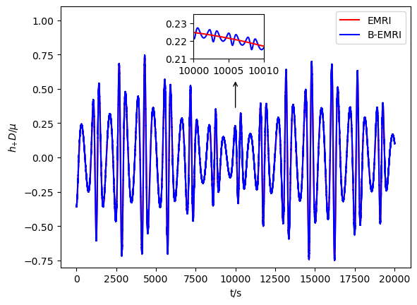
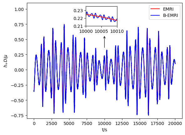
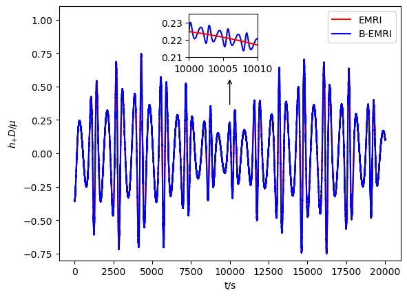
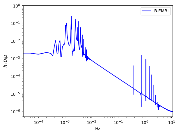
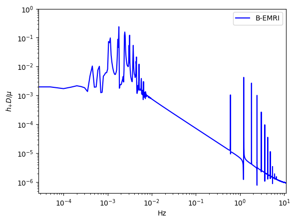
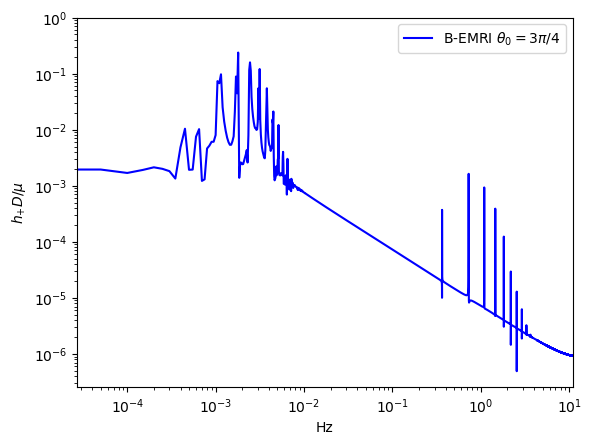
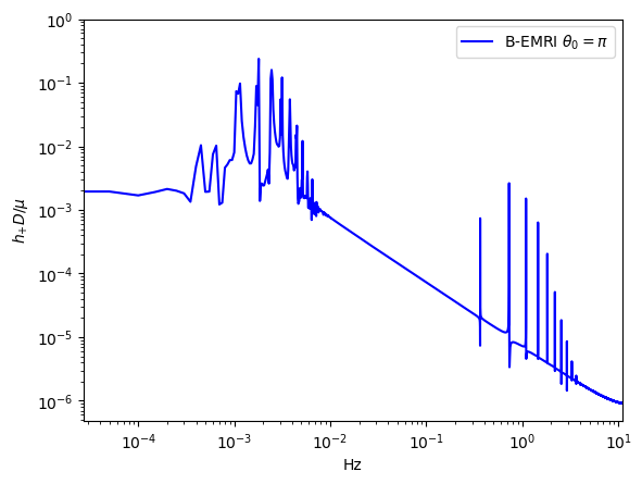
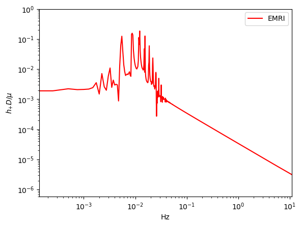
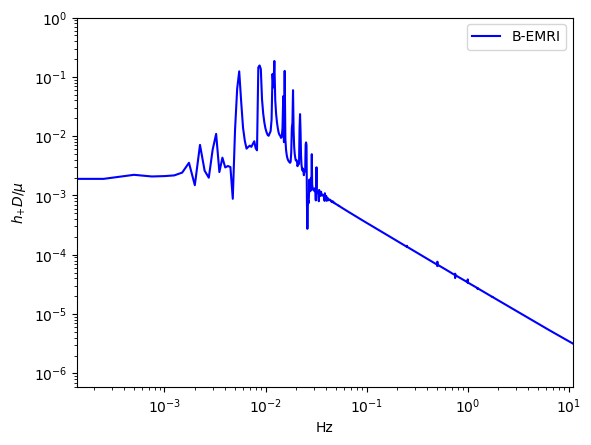
With all the results above, we are able to calculate the GW numerically with the NK method. In Figs.3-6, we exhibit the waveforms of EMRIs and B-EMRIs for different parameter selections. The orientation of the internal elliptic orbit plane is determined by the angles and , is fixed to be . The observer is supposed to be located at , , . From the figure we see that, the waveforms of B-EMRIs have the identical profile as that of EMRIs, but the waveforms of B-EMRIs have oscillations which are caused by the internal motion of the binary. We will analyze the waveforms in detail in the next section.
2.3 Gravito-electromagnetic force
The internal orbit is calculated by Newtonian dynamics in Eq. 13. It is interesting and important to consider the higher order corrections e.g. the Gravito-electromagnetic force effect [60]. Unlike single free-falling compact object which always locates at the origin of the free-fall frame (FFF), every compact objects of the binary system will not locate at the origin of FFF due to the internal interaction of binary. According to equivalence principle only at the origin of FFF the spacetime is flat, if there is departure from the origin gravity will play a role. So for the binary we take into account the gravitational effects caused by the departure from the origin of FFF. For simplicity, we consider a circular orbit on the equatorial plane in the following. The natural choice of FFF is Riemann normal coordinates
| (29) |
If , which is small compared to and , is neglected, the metric above can be rewritten as
| (30) |
where
| (31) | ||||
are the scalar and vector potentials of GEM fields. Analogous to the electromagnetic fields, the GEM force can be introduced
| (32) |
where
| (33) | ||||
In FFF the equations of motion of the compact object in binary system can be wriiten as
| (34) |
where label the compact objects which constitute the binary.

Although the equations of motion can be written in a simple form in FFF, it is not straightforward to calculate GEM force in FFF since Riemann tensor is conventionally derived in local non-rotating frame (LNRF). The transformations between the coordinates of LNRF () and BL coordinates are given by
| (35) | ||||
where . It’s shown Riemann tensor in LNRF takes very simple form[61, 62]. For circular orbit on the equatorial plane, the free-fall observer is moving in the direction with the speed[61]
| (36) |
where the upper signs refer to prograde orbits and the lower ones refer to retrograde orbits. The LNRF and the local inertial frame (LIF) are connected by a Lorentz transformation
| (37) |
where . Through the Lorentz transformation (37) Riemann tensor in LNRF can be transformed to the ones in LIF . If a free gyro placed at the origin of FFF, its spin axis is fixed in FFF, but in general the gyro will precess relative to the LNRF and LIF, so there exist rotation between LIF and FFF, the angular velocity is [63]. The tensors in LIF and the that in FFF are connected through a rotation transformation. The components of GEM force in FFF can be given in terms of that in LIF as
| (38) | ||||
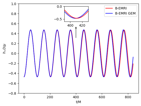
Substituting the GEM force (38) into the equations of motion (34) and solving the equations allows to obtain the positions of compact objects in FFF. Considering the orbit of origin of FFF is geodesic in external SBH spacetime, it’s straightforward to obtain the positions of compact objects of the binary in SBH spacetime, based on this one is able to calculate the GWs with the NK method. In Fig.7 we present the waveform of GW with and without taking into account GEM force.
3 Analysis of the waveforms
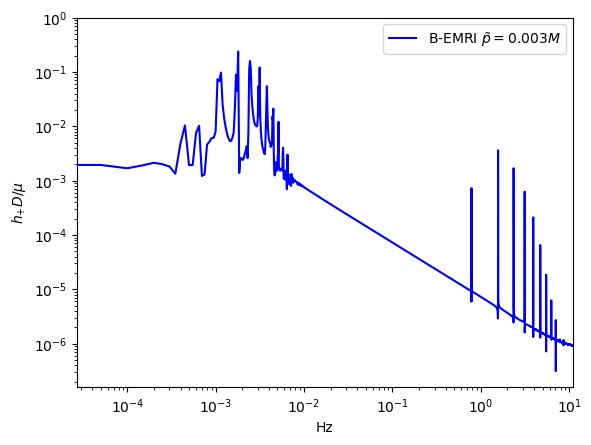
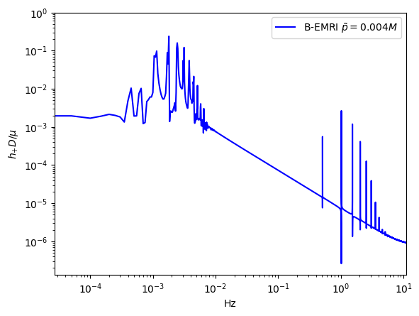
In this section, we compare the waveforms of B-EMRIs with that of EMRIs in detail. Furthermore, we investigate the modification of the waveform by considering the Gravito-electromagnetic (GEM) force effect and show that the dominated effect of GEM is a surplus phase shift. Fig.3 displays the waveforms of EMRIs and B-EMRIs with different masses. One sees that the profile of GWs of EMRIs and B-EMRIs are similar, but the details are distinct. For B-EMRIs, the gravitational waveforms possess small fluctuations. This is caused by the internal motions of the binary. We see, as mass increases, both the amplitudes and the frequency of the fluctuations increase. Fig.4 displays the the waveforms of EMRIs and B-EMRIs with different semi-latus rectum of the internal orbit. The figure shows that the smaller is, the larger the amplitude and the frequency of the fluctuation are, and vice versa. Since smaller corresponds to small cycle or higher frequency, amplitude of the fluctuation increases as decreases is expected.
Fig.5 displays the comparisons of the waveforms between EMRIs and B-EMRIs with different , which shows that, as increases the amplitude of fluctuation first decreases and then increases, especially when or the amplitude of fluctuation takes maximum value, i.e., when the rotation axis of the binary is parallel or anti-parallel to the rotation axis of the SBH, the waveforms of B-EMRIs and EMRIs take the most sharp distinction.
In Fig.6 the waveforms of EMRIs and B-EMRIs with SBH weighted are displayed. One sees that, since the central SBH is much heavier in this case, the amplitude of fluctuation generated by binary composed of compact objects weighted and is very tiny. This is because for heavier BH with parameter selection the cycle is much longer and frequency is much smaller. As displayed in Fig.3, like the case as mass increases the amplitude of fluctuation increases.


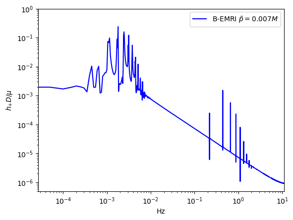
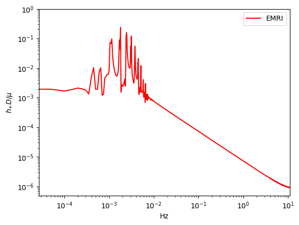
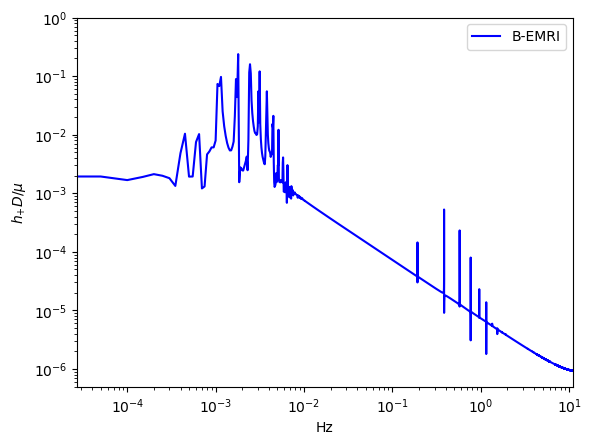
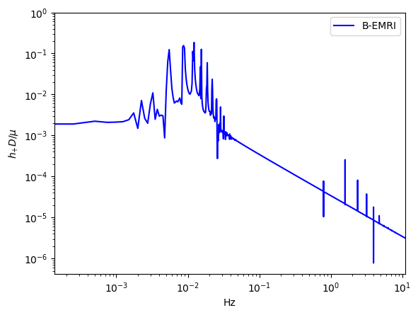
To compare the waveforms of B-EMRIs and EMRIs we analyse the waveforms in frequency domain. In Fig.8 we present the frequency spectrum of the waveforms in Fig.3. One sees that, in low frequency region the spectrum of B-EMRIs coincide with that of EMRIs. In high frequency region, only the B-EMRIs have non-vanishing amplitudes of gravitational signals. Further, as mass increases, the amplitudes of signals increase, and the more and more higher-frequency signals emerge. This result agrees with the waveforms in Fig.3, where it shows as mass increases the amplitude and frequency of the fluctuations become larger. This is because, on the one hand, the amplitude of GW is proportional to the mass of the source, on the other hand, as mass increases, the cycle decreases and the frequency increases. From the GW expression (15) we know, as frequency increases the amplitude of GW increases as well.

-
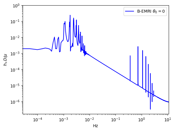
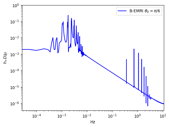
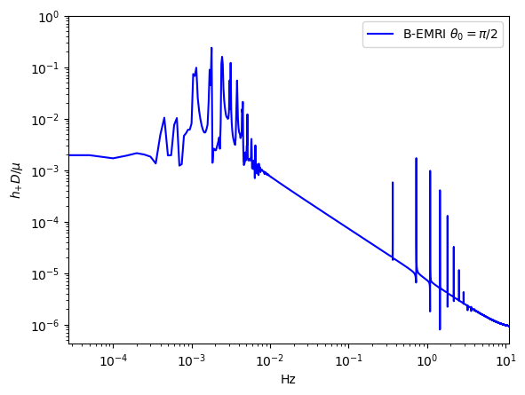
In Fig.9, we give the frequency spectrum of the GWs in Fig.4. We can see, as decreases, the amplitude of GW signal increases, and more and more high-frequency signals emerge, and vice versa. This agrees with what the waveform shows. Since the smaller is, the shorter the cycle is, and the higher the frequency is, so the amplitude of the signal increases. In Fig.10 we give the frequency spectrum of the waveforms in Fig.5 with distinct . We can see, for distinct , the frequency range is not significantly different. The amplitude of the signals with different frequency first decreases and then increases. For or , the amplitude of the signals takes the maximum value, which agrees with the waveforms in Fig.5.
When GEM force is taken into account, phase shift between the GW waveforms of B-EMRIs and that of EMRIs emerges, as shown in Fig.7. It’s sensitive and valuable to calculate mismatch of the two waveforms to quantify the distinction between them. The inner product of two signals is defined as
| (39) |
where and are the Fourier transformations of time-domain signals and
| (40) |
Here denotes the complex conjugate of a quantity, and in (41) is the one-sided noise power spectral density of LISA [59], which is significant for surveying the types of sources that can be detected by the LISA mission.
With the inner product defined in (39), the overlap of two signals is given by
| (41) |
Mismatch of two GW signals is defined as
| (42) |
There is a criterion that if two signals are distinguishable the mismatch and signal-noise-ratio (SNR) should satisfy[64, 65, 66, 67, 68]
| (43) |
where the SNR is defined as for a signal . For LISA, the SNR is taken to be [16]. Calculation shows for the two waveforms in the first panel of Fig.7 , for the two waveforms in the second panel of Fig.7 , which means when taking into account GEM force the waveforms of B-EMRIs are distinguishable from the waveforms of B-EMRIs that does not take into account GEM force, and are distinguishable from the waveforms of EMRIs as well.
4 Conclusion and Discussion
In this paper we study the GWs emanated from B-EMRIs which is composed of a central SBH and binary revolving around it. B-EMRIs are quite popular in the universe, and remarkable objects for GW detectors of next generation. We demonstrate that the waveform of B-EMRIs is distinctly different from that of EMRIs in frequency domain, and show that the mismatch can be effectively probed by the space-based GW detectors such as LISA, Taiji, and Tianqin. Our results will improve template construction for B-EMRIs and shed light on detection of GWs from B-EMRIs.
We solve the GW equations by taking into account the mass quadrupole, mass octupole and current quadrupole moments of the source. For the radiation reaction we take the hybrid 2nd order post-Newtonian approximation which is applicable to generic inclined-eccentric orbits. We plot the GW waveforms of B-EMRIs and compare the waveforms of B-EMRIs with that of EMRIs of single star. The results show that, the waveforms generated by single stellar-mass compact object share the same profile with the ones generated by binary compact objects, but the details of the waveforms of B-EMRIs exhibit fluctuations. The fluctuations are caused by internal motions of the binary. As masses of the compact objects of binary increase, the amplitudes and frequencies of the fluctuations increase. This is because, on the one hand, the amplitude of GW is proportional to the mass of the source. On the other hand, the increase of mass of gravitational source cause the decrease of cycle, so the frequency increases, which increases the amplitude further. We fix other parameters and only adjust the semi-latus rectum of internal orbits , the result shows that, as decreases, the amplitudes and frequencies of the fluctuations increase. This is because, as decreases, the cycle of internal motion decreases, the frequency increases, which causes the increase of amplitudes of GWs. We fix other parameters and adjust the angle between axes and , the results show that, when or the amplitudes of GW fluctuations caused by binary internal motions are larger than the cases when takes other values, which means when or the GWs of B-EMRIs are most easily distinguished from that of EMRIs.
For the binary on the equatorial plane of SBH, we further take in account GEM force and calculate the GWs of B-EMRIs. By comparing with both the waveforms of B-EMRIs that does not take into account GEM force and the waveforms of EMRIs, it’s easy to find there is phase shift between the related two waveforms.
To compare the GWs of EMRIs and B-EMRIs further we perform the frequency spectrum analysis. The results show that, at low-frequency region, the frequency spectrum of B-EMRIs coincide with that of EMRIs. At high-frequency region, the frequency spectrum of B-EMRIs and EMRIs are different. As masses of the binary increase, more high-frequency signals emerge, and the amplitudes of the GW signals increase, which agrees with the waveforms show us. We give the frequency spectrum of GWs generated by binary with distinct semi-latus rectum of internal orbits , the results show that, as decreases, more high-frequency signals emerge, and the amplitude of the GW signals increase, since smaller corresponds to shorter cycle and higher-frequency orbit motions, higher-frequency orbit motions generate GWs with higher amplitudes. If we adjust the angle between axes and , frequency spectrum show that when or the amplitudes of GWs are larger than that of GWs when takes other values, this agrees with what the waveforms show us as well. So the GW signals of B-EMRIs can be clearly distinguished from that of EMRIs through spectrum analysis, the GW signals generated by binary with larger mass, closer distance are more easily to be distinguished from that generated by single compact object. Moreover, when rotation axis of the binary is parallel or anti-parallel to that of the central SBH, the GW signals of B-EMRIs are more easily to be distinguished from that of EMRIs. When taking into account GEM force, we analyze the waveforms by calculating mismatch, calculation shows the GW waveforms of B-EMRIs are distinguishable from the waveforms of B-EMRIs that does not take into account GEM force and from the waveforms of EMRIs.

Appendix
The -dependent coefficients appear in Eq.(23) are given by
Acknowledgment
This work is supported by the National Key RD Program of China (no.2021YFC2203002), the National Natural Science Foundation of China Grants Nos. 12275106 and 12235019, and Natural Science Foundation of Shandong Province Nos.ZR2023MA014.
References
- [1] K. Akiyama et al. [Event Horizon Telescope], First M87 Event Horizon Telescope Results. VI. The Shadow and Mass of the Central Black Hole, Astrophys. J. Lett. 875, no.1, (2019) L6 [arXiv:1906.11243 [astro-ph.GA]].
- [2] K. Akiyama et al. [Event Horizon Telescope], First Sagittarius A* Event Horizon Telescope Results. VI. Testing the Black Hole Metric, Astrophys. J. Lett. 930, no.2, L17 (2022).
- [3] B. P. Abbott et al. [LIGO Scientific and Virgo], Observation of Gravitational Waves from a Binary Black Hole Merger, Phys. Rev. Lett. 116, no.6, 061102 (2016) [arXiv:1602.03837 [gr-qc]].
- [4] B. P. Abbott et al. [LIGO Scientific and Virgo], GW151226: Observation of Gravitational Waves from a 22-Solar-Mass Binary Black Hole Coalescence, Phys. Rev. Lett. 116, no.24, 241103 (2016) [arXiv:1606.04855 [gr-qc]].
- [5] S. Sigurdsson, Estimating the detectable rate of capture of stellar mass black holes by massive central black holes in normal galaxies, Class. Quant. Grav. 14, 1425-1429 (1997) [arXiv:astro-ph/9701079 [astro-ph]].
- [6] S. Sigurdsson and M. J. Rees, Capture of stellar mass compact objects by massive black holes in galactic cusps, Mon. Not. Roy. Astron. Soc. 284, 318 (1997) [arXiv:astro-ph/9608093 [astro-ph]].
- [7] S. A. Hughes, Evolution of circular, nonequatorial orbits of Kerr black holes due to gravitational wave emission. II. Inspiral trajectories and gravitational wave forms, Phys. Rev. D 64, 064004 (2001) [erratum: Phys. Rev. D 88, no.10, 109902 (2013)] [arXiv:gr-qc/0104041 [gr-qc]].
- [8] K. Glampedakis and D. Kennefick, Zoom and whirl: Eccentric equatorial orbits around spinning black holes and their evolution under gravitational radiation reaction, Phys. Rev. D 66, 044002 (2002) [arXiv:gr-qc/0203086 [gr-qc]].
- [9] P. Gupta, L. Speri, B. Bonga, A. J. K. Chua and T. Tanaka, Modeling transient resonances in extreme-mass-ratio inspirals, Phys. Rev. D 106, no.10, 104001 (2022) [arXiv:2205.04808 [gr-qc]].
- [10] L. Polcar, G. Lukes-Gerakopoulos and V. Witzany, Extreme mass ratio inspirals into black holes surrounded by matter, Phys. Rev. D 106, no.4, 044069 (2022) [arXiv:2205.08516 [gr-qc]].
- [11] C. Munna and C. R. Evans, Post-Newtonian expansion of the spin-precession invariant for eccentric-orbit nonspinning extreme-mass-ratio inspirals to 9PN and e16, Phys. Rev. D 106, no.4, 044058 (2022) [arXiv:2206.04085 [gr-qc]].
- [12] M. Kerachian, L. Polcar, V. Skoupý, C. Efthymiopoulos and G. Lukes-Gerakopoulos, Action-angle formalism for extreme mass ratio inspirals in Kerr spacetime, Phys. Rev. D 108, no.4, 044004 (2023) [arXiv:2301.08150 [gr-qc]].
- [13] T. Takahashi, H. Omiya and T. Tanaka, Evolution of binary systems accompanying axion clouds in extreme mass ratio inspirals, Phys. Rev. D 107, no.10, 103020 (2023) [arXiv:2301.13213 [gr-qc]].
- [14] L. M. Burko and G. Khanna, Self-force gravitational waveforms for extreme and intermediate mass ratio inspirals. II: Importance of the second-order dissipative effect, Phys. Rev. D 88, no.2, 024002 (2013) [arXiv:1304.5296 [gr-qc]].
- [15] K. Glampedakis, Extreme mass ratio inspirals: LISA’s unique probe of black hole gravity, Class. Quant. Grav. 22, S605-S659 (2005) [arXiv:gr-qc/0509024 [gr-qc]].
- [16] S. Babak, J. Gair, A. Sesana, E. Barausse, C. F. Sopuerta, C. P. L. Berry, E. Berti, P. Amaro-Seoane, A. Petiteau and A. Klein, Science with the space-based interferometer LISA. V: Extreme mass-ratio inspirals, Phys. Rev. D 95, no.10, 103012 (2017) [arXiv:1703.09722 [gr-qc]].
- [17] C. Munna and C. R. Evans, Eccentric-orbit extreme-mass-ratio-inspiral radiation: Analytic forms of leading-logarithm and subleading-logarithm flux terms at high PN orders, Phys. Rev. D 100, no.10, 104060 (2019) [arXiv:1909.05877 [gr-qc]].
- [18] T. G. Zi, J. D. Zhang, H. M. Fan, X. T. Zhang, Y. M. Hu, C. Shi and J. Mei, Science with the TianQin Observatory: Preliminary results on testing the no-hair theorem with extreme mass ratio inspirals, Phys. Rev. D 104, no.6, 064008 (2021) [arXiv:2104.06047 [gr-qc]].
- [19] K. Destounis, A. Kulathingal, K. D. Kokkotas and G. O. Papadopoulos, Gravitational-wave imprints of compact and galactic-scale environments in extreme-mass-ratio binaries, Phys. Rev. D 107, no.8, 084027 (2023) [arXiv:2210.09357 [gr-qc]].
- [20] T. Zi and P. C. Li, Probing the tidal deformability of the central object with analytic kludge waveforms of an extreme-mass-ratio inspiral, Phys. Rev. D 108, no.2, 024018 (2023) [arXiv:2303.16610 [gr-qc]].
- [21] L. Barack and C. Cutler, LISA capture sources: Approximate waveforms, signal-to-noise ratios, and parameter estimation accuracy, Phys. Rev. D 69, 082005 (2004) [arXiv:gr-qc/0310125 [gr-qc]].
- [22] T. Zi and P. C. Li, Gravitational waves from extreme-mass-ratio inspirals around a hairy Kerr black hole, Phys. Rev. D 108, no.8, 084001 (2023) [arXiv:2306.02683 [gr-qc]].
- [23] N. Dai, Y. Gong, Y. Zhao and T. Jiang, Extreme mass ratio inspirals in galaxies with dark matter halos, [arXiv:2301.05088 [gr-qc]].
- [24] Z. Pan, H. Yang, L. Bernard and B. Bonga, Resonant dynamics of extreme mass-ratio inspirals in a perturbed Kerr spacetime, Phys. Rev. D 108, no.10, 104026 (2023) [arXiv:2306.06576 [gr-qc]].
- [25] C. Zhang, Y. Gong, D. Liang and B. Wang, Gravitational waves from eccentric extreme mass-ratio inspirals as probes of scalar fields JCAP 06, 054 (2023) [arXiv:2210.11121 [gr-qc]].
- [26] D. Liang, R. Xu, Z. F. Mai and L. Shao, Probing vector hair of black holes with extreme-mass-ratio inspirals Phys. Rev. D 107, no.4, 044053 (2023) [arXiv:2212.09346 [gr-qc]].
- [27] C. M. Will, Gravitational Radiation from Binary Systems in Alternative Metric Theories of Gravity: Dipole Radiation and the Binary Pulsar, Astrophys. J. 214, 826-839 (1977)
- [28] C. M. Will and H. W. Zaglauer, Gravitational Radiation, Close Binary Systems, and the Brans-dicke Theory of Gravity, Astrophys. J. 346, 366 (1989)
- [29] E. Barausse and K. Yagi, Gravitation-Wave Emission in Shift-Symmetric Horndeski Theories, Phys. Rev. Lett. 115, no.21, 211105 (2015) [arXiv:1509.04539 [gr-qc]].
- [30] R. Xu, Y. Gao and L. Shao, Neutron stars in massive scalar-Gauss-Bonnet gravity: Spherical structure and time-independent perturbations, Phys. Rev. D 105, no.2, 024003 (2022) [arXiv:2111.06561 [gr-qc]].
- [31] J. Tan, J. d. Zhang, H. M. Fan and J. Mei, Constraining the EdGB Theory with Extreme Mass-Ratio Inspirals, [arXiv:2402.05752 [gr-qc]].
- [32] J. Gair and N. Yunes, Approximate Waveforms for Extreme-Mass-Ratio Inspirals in Modified Gravity Spacetimes, Phys. Rev. D 84, 064016 (2011) [arXiv:1106.6313 [gr-qc]].
- [33] M. Rahman, S. Kumar and A. Bhattacharyya, Gravitational wave from extreme mass-ratio inspirals as a probe of extra dimensions, JCAP 01, 046 (2023) 5doi:10.1088/1475-7516/2023/01/046 [arXiv:2212.01404 [gr-qc]].
- [34] T. Zi, Z. Zhou, H. T. Wang, P. C. Li, J. d. Zhang and B. Chen, Analytic kludge waveforms for extreme-mass-ratio inspirals of a charged object around a Kerr-Newman black hole, Phys. Rev. D 107, no.2, 023005 (2023) [arXiv:2205.00425 [gr-qc]].
- [35] S. C. Yang, R. D. Tang, X. Y. Zhong, Y. H. Zhang and W. B. Han, Recognizing the constitution of small bodies in extreme-mass-ratio inspirals by gravitational waves, [arXiv:2209.01110 [gr-qc]].
- [36] C. Zhang and Y. Gong, Detecting electric charge with extreme mass ratio inspirals, Phys. Rev. D 105, no.12, 124046 (2022) [arXiv:2204.08881 [gr-qc]].
- [37] L. V. Drummond, A. G. Hanselman, D. R. Becker and S. A. Hughes, Extreme mass-ratio inspiral of a spinning body into a Kerr black hole I: Evolution along generic trajectories, [arXiv:2305.08919 [gr-qc]].
- [38] Y. Mino, M. Shibata and T. Tanaka, Gravitational waves induced by a spinning particle falling into a rotating black hole, Phys. Rev. D 53, 622-634 (1996) [erratum: Phys. Rev. D 59, 047502 (1999)]
- [39] B. Toshmatov, O. Rahimov, B. Ahmedov and D. Malafarina, Motion of spinning particles in non asymptotically flat spacetimes, Eur. Phys. J. C 80, no.7, 675 (2020) [arXiv:2003.09227 [gr-qc]].
- [40] G. A. Piovano, A. Maselli and P. Pani, Extreme mass ratio inspirals with spinning secondary: a detailed study of equatorial circular motion, Phys. Rev. D 102, no.2, 024041 (2020) [arXiv:2004.02654 [gr-qc]].
- [41] S. Drasco and S. A. Hughes, Gravitational wave snapshots of generic extreme mass ratio inspirals, Phys. Rev. D 73, no.2, 024027 (2006) [erratum: Phys. Rev. D 88, no.10, 109905 (2013); erratum: Phys. Rev. D 90, no.10, 109905 (2014)] [arXiv:gr-qc/0509101 [gr-qc]].
- [42] S. A. Hughes, The Evolution of circular, nonequatorial orbits of Kerr black holes due to gravitational wave emission, Phys. Rev. D 61, no.8, 084004 (2000) [erratum: Phys. Rev. D 63, no.4, 049902 (2001); erratum: Phys. Rev. D 65, no.6, 069902 (2002); erratum: Phys. Rev. D 67, no.8, 089901 (2003); erratum: Phys. Rev. D 78, no.10, 109902 (2008); erratum: Phys. Rev. D 90, no.10, 109904 (2014)] [arXiv:gr-qc/9910091 [gr-qc]].
- [43] C. Cutler, D. Kennefick and E. Poisson, Gravitational radiation reaction for bound motion around a Schwarzschild black hole, Phys. Rev. D 50, 3816-3835 (1994).
- [44] T. Tanaka, M. Shibata, M. Sasaki, H. Tagoshi and T. Nakamura, Gravitational wave induced by a particle orbiting around a Schwarzschild black hole, Prog. Theor. Phys. 90, 65-84 (1993).
- [45] M. Shibata, Gravitational Waves Induced by a Particle Orbiting around a Rotating Black Hole: Effect of Orbital Precession,
- [46] H. Tagoshi, Post Newtonian expansion of gravitational waves from a particle in slightly eccentric orbit around a rotating black hole, Prog. Theor. Phys. 93, 307-333 (1995) [erratum: Prog. Theor. Phys. 118, 577-579 (2007)]
- [47] E. Poisson, Gravitational radiation from a particle in circular orbit around a black hole. 1: Analytical results for the nonrotating case, Phys. Rev. D 47, 1497-1510 (1993).
- [48] C. Cutler, E. Poisson, G. J. Sussman and L. S. Finn, Gravitational radiation from a particle in circular orbit around a black hole. 2: Numerical results for the nonrotating case, Phys. Rev. D 47, 1511-1518 (1993).
- [49] T. Apostolatos, D. Kennefick, E. Poisson and A. Ori, Gravitational radiation from a particle in circular orbit around a black hole. 3: Stability of circular orbits under radiation reaction, Phys. Rev. D 47, 5376-5388 (1993).
- [50] E. Poisson, Gravitational radiation from a particle in circular orbit around a black hole. 4: Analytical results for the slowly rotating case, Phys. Rev. D 48, 1860-1863 (1993).
- [51] E. Poisson and M. Sasaki, Gravitational radiation from a particle in circular orbit around a black hole. 5: Black hole absorption and tail corrections, Phys. Rev. D 51, 5753-5767 (1995) [arXiv:gr-qc/9412027 [gr-qc]].
- [52] H. Tagoshi and M. Sasaki, Post Newtonian expansion of gravitational waves from a particle in circular orbit around a Schwarzschild black hole, Prog. Theor. Phys. 92, 745-772 (1994) [arXiv:gr-qc/9405062 [gr-qc]].
- [53] M. Shibata, M. Sasaki, H. Tagoshi and T. Tanaka, Gravitational waves from a particle orbiting around a rotating black hole: PostNewtonian expansion, Phys. Rev. D 51, 1646-1663 (1995) [arXiv:gr-qc/9409054 [gr-qc]].
- [54] S. Babak, H. Fang, J. R. Gair, K. Glampedakis and S. A. Hughes, ’Kludge’ gravitational waveforms for a test-body orbiting a Kerr black hole, Phys. Rev. D 75, 024005 (2007) [erratum: Phys. Rev. D 77, 04990 (2008)] [arXiv:gr-qc/0607007 [gr-qc]].
- [55] F. D. Ryan, Effect of gravitational radiation reaction on circular orbits around a spinning black hole, Phys. Rev. D 52, R3159-R3162 (1995) [arXiv:gr-qc/9506023 [gr-qc]].
- [56] F. D. Ryan, Effect of gravitational radiation reaction on nonequatorial orbits around a Kerr black hole, Phys. Rev. D 53, 3064-3069 (1996) [arXiv:gr-qc/9511062 [gr-qc]].
- [57] J. R. Gair and K. Glampedakis, Improved approximate inspirals of test-bodies into Kerr black holes, Phys. Rev. D 73, 064037 (2006) [arXiv:gr-qc/0510129 [gr-qc]].
- [58] B. Carter, Axisymmetric Black Hole Has Only Two Degrees of Freedom, Phys. Rev. Lett. 26, 331-333 (1971).
- [59] T. Robson, N. J. Cornish and C. Liu, The construction and use of LISA sensitivity curves, Class. Quant. Grav. 36, no.10, 105011 (2019) [arXiv:1803.01944 [astro-ph.HE]].
- [60] X. Chen and Z. Zhang, “Binaries wandering around supermassive black holes due to gravitoelectromagnetism,” Phys. Rev. D 106, no.10, 103040 (2022) [arXiv:2206.08104 [astro-ph.HE]].
- [61] J. M. Bardeen, W. H. Press and S. A. Teukolsky, “Rotating black holes: Locally nonrotating frames, energy extraction, and scalar synchrotron radiation,” Astrophys. J. 178, 347 (1972).
- [62] S. Chandrasekhar, The mathematical theory of black hole[M]. (1983).
- [63] W. Rindler and V. Perlick, “Rotating coordinates as tools for calculating circular geodesics and gyroscopic precession,” Gen.Rel.Grav. 22, 1067 (1990).
- [64] L. V. Drummond, P. Lynch, A. G. Hanselman, D. R. Becker and S. A. Hughes, Extreme mass-ratio inspiral and waveforms for a spinning body into a Kerr black hole via osculating geodesics and near-identity transformations, [arXiv:2310.08438 [gr-qc]].
- [65] H. Yu, J. Roulet, T. Venumadhav, B. Zackay and M. Zaldarriaga, Accurate and efficient waveform model for precessing binary black holes, Phys. Rev. D 108, no.6, 064059 (2023) [arXiv:2306.08774 [gr-qc]].
- [66] M. Pürrer, Frequency domain reduced order models for gravitational waves from aligned-spin compact binaries Class. Quant. Grav. 31, no.19, 195010 (2014) [arXiv:1402.4146 [gr-qc]].
- [67] F. Ohme, Analytical meets numerical relativity - status of complete gravitational waveform models for binary black holes, Class. Quant. Grav. 29, 124002 (2012) [arXiv:1111.3737 [gr-qc]].
- [68] P. Lynch, M. van de Meent and N. Warburton, Eccentric self-forced inspirals into a rotating black hole, Class. Quant. Grav. 39, no.14, 145004 (2022) [arXiv:2112.05651 [gr-qc]].