Gravitationally Bound Bose Condensates with Rotation
Abstract
We develop a self-consistent, Gravitoelectromagnetic (GEM) formulation of a slowly rotating, self-gravitating and dilute Bose-Einstein condensate (BEC), intended for astrophysical applications in the context of dark matter halos. GEM self-consistently incorporates the effects of frame dragging to lowest order in via the Gravitomagnetic field. BEC dark matter has attracted attention as an alternative to Cold dark matter (CDM) and Warm dark matter (WDM) for some time now. The BEC is described by the Gross-Pitaevskii-Poisson (GPP) equation with an arbitrary potential allowing for either attractive or repulsive interactions. Owing to the difficulty in obtaining exact solutions to the GEM equations of motion without drastic approximations, we employ the variational method to examine the conditions under which rotating condensates, stable against gravitational collapse, may form in models with attractive and repulsive quartic interactions. We also describe the approximate dynamics of an imploding and rotating condensate by employing a collective coordinate description in terms of the condensate radius.
I Introduction
The standard (CDM) model for the matter-energy distribution of the universe posits that the universe consists primarily of a cosmological constant () plus cold dark matter (CDM). It has been fairly successful on scales larger than the typical galactic scale ( 50 kpc) but appears to make predictions that are somewhat inconsistent with observations on smaller scales ( 50 kpc). In this model, only about 4% of the matter-energy budget of the universe is ordinary baryonic matter as we know it, 22% is non-baryonic dark matter (DM) and the rest is a mysterious form of energy (dark energy, DE), which appears to be reasonably well described by a positive cosmological constant rea98 ; pea99 ; eea05 . The model has provided a useful framework for understanding structure formation via density fluctuations and has had some success in explaining the power spectrum of the mass fluctuations in the Cosmic Microwave Background (CMB) radiation kea11 ; hea12 ; pla15 , the large scale structure san12 ; and12 and the large scale structure of DM halos wal09 ; vik09 ; new12 . On smaller scales, however, numerical simulations dc91 ; fp94 ; mo94 ; nfw96 predict unobserved cusps in the central dark matter density profiles of galactic halos. On the contrary, observations of rotation curves prefer cored distribution profiles i.e., having a nearly constant DM density near the center gts07 ; ohea07 ; dea09 ; ns13 . Furthermore, because of the hierarchical growth of structure in the CMB models, they predict an excess of low mass sub-halos within the galaxy as well as an excess of massive sub-halos, capable of being bright enough to be observed as satellite galaxies kkvp99 ; mgea99 ; swea08 ; bs09 ; bkbk11 ; fw12 ; wbgkn15 . Other problems also indicate that the CDM model may be in need of tuning: for example, pure disk (bulge free) galaxies cannot be simulated in this model gbea10 ; kdbc10 and some anomalies between the CMB mass power spectrum obtained by the Sloan Digital Sky Survey (SDSS) and that predicted by the CDM paradigm have been found bbk17 .
A proposed alternative to CDM is a light boson whose mass is small enough that its critical temperature is well above that of the CMB. This ensures that a significant fraction of the bosons settle in the ground state and form a BEC kaup68 ; rb69 ; wt83 ; bgz84 ; imr90 ; bh07 . If the particle mass is small enough so that its de Broglie wavelength is on the order of the typical galactic scale (say kpc), smaller scale structure will be suppressed while on the large scale it would be virtually indistinguishable from CDM mst83 ; prs90 ; sjs94 ; hbg00 ; jg00 ; pjp00 ; ab05 ; phc11 ; scb14 ; ds14 ; lds14 ; hoea17 . Such low masses are not inconceivable, considering that ultra-light bosons (of mass even as low as ev) are predicted by multidimensional cosmology and string theory hw96 ; gz97 ; add99 ; ar10 . Larger particle masses lead to smaller, asteroid sized, stable, BEC structures (one example is the QCD axion), which, in sufficient numbers, could form one component of DM csw86 ; kmz85 ; bsk92 ; sk94 ; ssk96 ; kss99 ; sg01 ; krs04 ; k08 ; bb11 ; ghp15 ; esvw14 ; elsw16 ; lpt17 ; phc17 ; hmea17 ; sh17 . Of interest in either case, but particularly for large halos, is the description of rotating condensates sds95 ; mmea99 ; rds12 ; ds16 .
In this work, we provide a Gravitoelectromagnetic (GEM) description of gravitationally bound, non-relativistic, rotating BECs. It is not our intention to obtain exact solutions of the equations of motion. Instead, we analyze the effects of the rotation by applying the variational method. The variational method is widely used in the study of BECs, in condensed matter physics bist97 ; ps08 and was adopted early in the Boson star literature (eg. phc11 ) as well, owing to the difficulty in obtaining solutions of the coupled system of equations.
In section II, beginning with the relativistic Klein-Gordon field in a weak, axisymmetric gravitational field, we set up the effective Gross-Pitaevskii-Poisson (GPP) action, describing a BEC cloud with rotation and including the gravitational action appropriate to an axisymmetric spacetime in the weak field approximation. In section III, we describe stable configurations by applying the variational method with a single Gaussian Vortex ansatz appropriate to rotating BEC clouds. In section IV we examine the problem of vortex collapse and we summarize our results in section V.
II Action
As the candidate field for BEC halos is generally taken to be a light, but not massless, scalar field, we begin with the action for a complex scalar field in a curved background spacetime, , where
| (1) |
and is an arbitrary potential, which we take to be of the form
| (2) |
This action is supplemented by the gravitational action
| (3) |
linearized about flat space, taking .
II.1 The GPP Action
In the weak field approximation tp10 ; sc16 , where , if we set , where is the trace of , then the scalar field action can be written as the sum of three terms,
| (4) |
to linear order in . The zeroeth order action, , is the action in (1), but on a flat background. We will call the trace term and the second correction term . In the non-relativistic limit, the field can be described by a complex wavefunction according to
| (5) |
which, at low temperatures, describes a condensed, -particle state and will be normalized as in what follows. We will also take the scalar field potential to be of the form
| (6) |
Expanding the zeroeth order action in the non-relaivistic limit, one finds
| (7) |
where we have dropped terms quadratic in , using the fact that, in the non-relativistic approximation, the difference between the total energy and the rest mass energy is supposed to be small. In the same approximation,
| (8) |
Assuming the gravitational field is weak (), this term may therefore be dropped, as also the last term in the expansion of ,
| (9) | |||||
| (11) | |||||
| (13) |
If we call , , then this correction term looks like
| (14) |
where is the gravitational potential energy (to be obtained from the Einstein equations) and
| (15) |
is the scalar current. Putting everything together, the non-realtivistic, weak field GPP action for the scalar field is
| (16) |
The third term in the action above represents the self-interaction of the non-relativistic field, the fourth term represents its interaction with the gravitational field and the last term is the gravitomagnetic term, which incorporates frame dragging.
The non-relativistic action may be put in a more suggestive form if we define and the “covariant” derivative
| (17) |
Then,
| (18) |
and
| (19) |
upon dropping terms that are quadratic in the gravitational field. Thus our action reads,
| (20) |
so, in the weak field limit, the interaction of the scalar field with the gravitational field has the (well-known) form of an “electromagnetic” coupling.
II.2 The Gravitational Action
Turning to the gravitational part of the action, we first examine the Einstein equations of motion to determine the general form of the metric. It is convenient to work in the harmonic gauge, defining and imposing the condition . The Einstein tensor is and Einstein’s equations are
| (21) |
The gauge condition, tells us that the stress tensor is conserved on a flat background, so is to be evaluated for the field on a flat background,
| (22) |
In the non-relativistic limit, keeping only leading order terms, we find
| (23) | |||||
| (24) | |||||
| (25) |
This shows that we can take . In this case, . If we take then and . The remaining metric coefficients are
| (26) |
and the line element,
| (27) |
is subject to the gauge conditions,
| (28) |
In the non-relativistic limit, we may ignore the term , so our gauge conditions become .
To set up the total action it is convenient to compare the line element in (27) to the standard line element of Arnowitt, Deser and Misner (ADM) adm62
| (29) |
and write the bulk Lagrangian for the gravitational field in terms of the lapse function, , the shift, , the first fundamental form, , the intrinsic curvature scalar of spatial hypersurfaces, , and the extrinsic curvature (of spatial hypersurfaces), ,
| (30) |
where is the trace of . This gives us the lapse, shift and first fundamental form respectively in linear approximation,
| (31) | |||
| (32) | |||
| (33) |
from which we find the intrinsic curvature of the spatial hypersurfaces up to second order
| (34) |
and, up to first order, the extrinsic curvature
| (35) |
where we have defined . In this approximation, the trace of the extrinsic curvature, vanishes by virtue of the gauge condition. After some algebra, we find the gravitational action
| (36) |
where . The resulting total effective action,
| (37) |
now allows us to use the non-linear Schroedinger equation to describe large scale structure, so long as is interpreted as a Schroedinger field, normalized to the particle number, as mentioned earlier.
II.3 Equations of Motion
Extremizing the action in (37) with respect to variations in and employing the gauge conditions gives non-linear Schroedinger equation for
| (38) |
where is the transport derivative, which takes into account frame dragging due to the rotation. Likewise, varying and give
| (39) |
(employing the gauge condition) and
| (40) |
up to first order. These are readily solved by
| (41) | |||
| (42) | |||
| (43) |
respectively.
It is often useful to treat the BEC as a superfluid. We now consider the hydrodynamic analogy by employing the Madelung transformation m27 to rewrite equation (38). Setting phc11 ; bh07 ; phc16
| (44) |
where is the number density of particles and is the real action. By comparing the real and imaginary parts of the Schroedinger equation for we find
| (45) | |||
| (46) | |||
| (47) |
where is the “quantum potential”
| (48) |
If we introduce the velocity field, , then the first of the above equations,
| (49) |
has the form of a continuity equation. The second can also be put in an interesting form: write it as
| (50) |
and notice that is irrotational, so implying that . Likewise , therefore
| (51) |
where represents the mass density of the BEC and is the pressure given by
| (52) |
This is the general form of the equation of state. For example, for quartic interactions, , we find bh07
| (53) |
Thus, not surprisingly, a repulsive interaction () leads to a positive pressure and an attractive interaction () to a negative pressure. The effect of frame dragging is contained in the transport derivative, . In terms of the particle density and real action, the gravitational potential and shift are given by
| (54) | |||
| (55) | |||
| (56) |
respectively.
III Stable Configurations
(Meta)stable, rotating BEC configurations may be obtained by extremizing the total energy of the system, which, according to (37) will be given by
| (57) |
Introducing a length parameter, , a general ansatz for representing a rotating condensate in spherical coordinates would be
| (58) |
where is a normalization, is the non-relativistic chemical potential associated with the BEC, are integers, , are real functions of and are the spherical harmonics. In what follows, we will treat as a variational function. Here is a variational parameter. We hold the particle number and the total angular momentum fixed in the variational computation.
III.1 The Total Energy
For simplicity, we will analyze the situation when all particles are in the eigenstate of angular momentum, i.e., we take
| (59) |
The procedure below can be extended to arbitrary angular momentum states. The normalization condition gives,
| (60) |
where is the number of bosons in the BEC and . To find an expression for , we use the expansion of the Green function in spherical harmonics with vanishing boundary conditions at the origin and at infinity,
| (61) |
and find
| (64) | |||||
Now from (43) it follows that only survives (in this stationary state), and
| (65) |
Putting these results into (57), and taking, for simplicity, quartic interactions of arbitrary sign, , we find the four terms in the total energy to be
| (66) | |||||
| (68) | |||||
| (72) | |||||
| (74) |
where is a dimensionless variable. The second term in the integral in the expression for the kinetic energy, , represents the contribution of the azimuthal motion of the condensate. and are the contributions of the gravitational field. These expressions may be put into simpler form in terms of the coefficients
| (75) | |||
| (76) | |||
| (77) | |||
| (78) | |||
| (79) | |||
| (80) | |||
| (81) |
We find
| (82) | |||||
| (86) | |||||
does not include the rest mass energy, , of the condensate and the total energy can be written as . If is the binding energy per particle, then . We can therefore identify . In fact, using previous results esvw14 , let us define the dimensionless parameters and by
| (87) |
where is the Planck mass. Then the binding energy per unit mass may be given as,
| (88) |
where
| (89) | |||
| (90) | |||
| (91) |
The coefficient characterizes the contribution of the gravitational potential energy to the total energy and is negative and represents the contribution of the kinetic energy of the bosons. The effects of the rotation are contained in a contribution to the kinetic energy through the coefficient in and in the last term in the expression for , which combines the contributions of the scalar potential and frame dragging. This term is proportional to , where is a dimensionless parameter, , characterizing the strength of the self interactions.
III.2 Minimum Energy Configuration
The extrema of in (88) are readily found to be given by
| (92) |
assuming it is real, i.e., provided that when . In what follows, we set
| (93) | |||||
| (94) |
where the parameters , and are obtained from the constants defined in (91), viz.,
| (95) | |||
| (96) | |||
| (97) | |||
| (98) | |||
| (99) |
The first , , characterizes the strength of the gravitational interaction, the second, , characterizes the strength of the self interaction and the last, , the effect of the frame dragging. In terms of these, the dimensionless equilibrium radius is
| (100) |
For it to exist, we must require the quantity under the radical to be non-negative. If the kinetic energy of the bosons is ignored, as in the Thomas-Fermi approximation, approaches zero and the equilibrium radius approaches a constant independent of the number of particles. In the absence of rotation () this equilibrium is possible only for repulsive self interactions. If one does not ignore the kinetic energy of the bosons then the equilibrium radius decreases with increasing .
When an absolute minimum of the energy exists, as the interactions together with the rotations are able to stabilize the condensate. When only attractive interactions are permitted and the energy of the system is unbounded from below, but we have found a local minimum in (100), not an absolute minimum, of the energy. This local minimum exists only when the number of particles is below a certain critical value, , which will be determined below. It is important to discuss the validity of this solution.
There are three criteria that it must satisfy in order to be self consistent, the first two arising from the GEM approximation. First, the de Broglie wavelength of the bosons should be much larger than their Compton wavelength to ignore special relativistic corrections. Second, the size of the condensate at the minimum has to be much greater than the Schwarzschild radius of the corresponding mass, to justify not using general relativistic corrections. The impact of these two conditions on the range of the parameters is determined below and the conditions are satisfied by the examples we give. When the energy is unbounded from below (in the case , ) the local minimum we have found could be unstable. This can be avoided if additional stabilizing terms exist in the effective potential (as is the case for QCD axions, where the effective potential is given by the Bessel function esvw14 ). Irrespective of whether there is a stabilization term, the configuration at the local minimum could be a viable state, provided it has a lifetime greater than the age of the universe. This would occur if the probability of tunneling out of it is sufficiently small. The lifetime of metastable BECs formed by bosonic atoms with attractive interactions, confined by a harmonic trap, was estimated using instanton methods in st97 ; frar99 . One can use similar techniques to compute the lifetimes of gravitationally bound BEC systems against tunneling out of the metastable local minimum state. The result is that the tunneling rate behaves approximately as , where is the number of particles and is the WKB expression for the exponent of the tunneling rate. In the case of an astrophysical BEC, the number of particles is very large ( – ) and the WKB expression, , is not vanishingly small unless the fraction is commensurately close to unity. Thus so long as the lifetime of the metastable state grows exponentially with the particle number.
III.2.1
If there is an absolute minimum of the energy and either or
| (101) |
For attractive self-interactions (), rotation provides a stabilization mechanism. In the absence of rotation (), is possible only for repulsive interactions.
So long as , the number of particles, , and the interaction strength, , are limited only by the GEM approximation. As mentioned, we obtain a criterion for the validity of the non-relativistic approximation by requiring that the de Broglie wavelength of the bosons, , is much larger than the Compton wavelength, . As the de Broglie wavelength is roughly the typical size of the condensate, which is on the order of the scale factor, , for a BEC and, from (87), , it follows that the condition for the non-relativistic approximation to hold is
| (102) |
To justify not including higher order general relativistic effects one also wants a stable configuration whose equilibrium radius is much larger than the Schwarzschild radius, , so requiring that , we find
| (103) |
which places an upper limit on the particle number for any given value of .
It will be seen from (102) and (103) that, for attractive self-interactions, the weak gravity approximation holds only for condensates with small because is bounded from above according to (101). On the contrary, there is no such restriction on for repulsive interactions as can be arbitrarily large csw86 . As mentioned, in this case (100) represents an absolute minimum of the energy. Increasing the particle number, , also increases the strength of the gravitational attraction, therefore the radius of the system decreases with increasing . In the limit of large (repulsive self interactions) the system approaches the equilibrium radius,
| (104) |
III.2.2
If the energy is not bounded from below, but there is a local minimum of the energy. This case is only possible when
| (105) |
The condition for the validity of the non-relativistic approximation is (102), the same as in the case above. As can be arbitrarily large, this condition can always be verified. The energy is not bounded from below, but a local minimum exists provided that there is an an upper limit on the number
| (106) |
This therefore defines a critical number of particles above which there is no metastable configuration. The local equilibrium radius, which can now be written as
| (107) |
continues to decrease with increasing , so the smallest metastable condensate size occurs for . The existence of a minimum size (maximum number of particles) for the case of negative self-interactions can be understood as follows: for an equilibrium solution it is necessary for the inward gravitational and self interaction pressures to be balanced by the outward quantum pressure. This condition was used in ds16 to estimate the mass and radius of a non-rotating axion drop. They found an upper bound on the drop mass (as previously determined by Chavanis phc11 ) as well as the virial relation between the radius and mass of an object supported against gravity by pressure.
Finally, to consistently ignore general relativistic corrections, we ask that is small enough so that the equilibrium radius remains much larger than the Schwarzschild radius. This gives
| (108) |
and is the critical radius.
III.3 Single Vortex Ansatz
We can get a rough idea of the size of the rotating condensates by taking a variational approach phc11 ; ps08 ; rds12 ; elsw16 . This approach is known to be in good agreement with more precise (numerical) analyses kaup68 ; rb69 ; bb11 ; esvw14 ; dc11 ; eknw15 ; ps08 and requires some ansatz for the function . We ask for a trial wavefunction that behaves as a vortex of width and that is continuous everywhere. As a trial wave function, it is not required to be a solution of the equations of motion. Continuity at the origin suggests that, as approaches zero, should behave as , where . We therefore take
| (109) |
so that the wavefunction in cylindrical coordinates has the form
| (110) |
where is the cylindrical radius. The gravitational potential becomes
| (113) | |||||
and we find
| (114) | |||||
| (115) | |||||
| (116) | |||||
| (117) |
When , the conditions for the validity of the GEM approximation are (102) and (103),
| (118) | |||
| (119) | |||
| (120) |
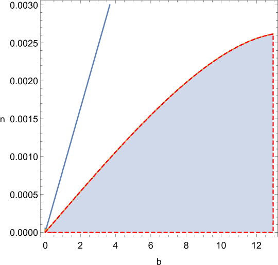
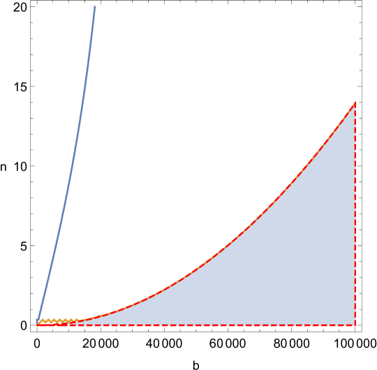
These conditions can be met by small condensates with attractive interactions and a suitably limited value of (). For repulsive interactions there is no upper limit on and large condensates are possible. The shaded regions in figures 2 and 2 represent the portion of the parameter space satisfying these conditions for the case of attractive interactions (figure 2) and repulsive interactions (figure 2). In each case, the trustworthy portion of the parameter space is limited by the second inequality in (120).
When only a metastable state may exist. The critical (maximum possible) number of bosons is
| (121) |
and the minimum possible equilibrium radius is given by the limit as ,
| (122) |
The two conditions (102) and (108) for the validity of the GEM approximation can therefore be stated as
| (123) | |||
| (124) | |||
| (125) |
As there is no upper limit on , they are readily met so long as is sufficiently large. In addition, to ensure a large lifetime, the actual mass of the BEC cannot be too close to its maximum mass, i.e., the fraction should not be too close to unity.
The parameters and of the BEC cloud are uniquely determined by the size of the self-interaction, , so the length scale, , and the total mass, depend only on the strength of the self-interaction and the particle mass.
III.4 Asteroid vs. Galaxy Size Halos
As an example, we consider the condensates formed by particles of mass and interaction strength typical of the QCD axion, ev and , where the axion decay constant is taken to be roughly . QCD axions have attractive interactions and the size of indicates that we are considering the case . From (87) we find that
| (126) |
with a total mass of kg. We also find the critical length scale associated with the ball
| (127) |
The Compton wavelength of the eV boson is about 0.02 m, which gives the radius as about km. The radius inside of which about 99.9% of the matter is confined, denoted by , is roughly 3.5 times this radius, so we find km.
Continuing with attractive self-interactions and assuming that , (106) suggests that we take the maximum (critical) size to be approximately independent of . Then is also approximately independent of and the dependence of and on and is simple. Using (87) one finds that the particle mass and interaction strength required to produce a desired value of and are given by
| (128) |
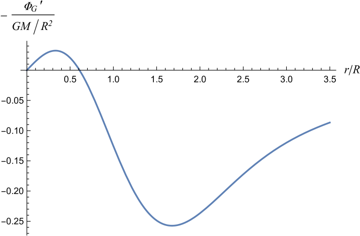
Taking kpc, and a mass of roughly three times that of the visible galaxy, kg, we find eV and . The condensate continues to be non-relativistic, satisfying the condition , with a total angular momentum of Js, which is comparable to that of the luminous matter cabe15 . For the vortex wavefunction in (109), however, the gravitational force in the equatorial plane, , is outward directed up to a distance of about (see figure (3)). This can be attributed to the shape of the density profile which vanishes at the center and increases until about as one moves outward in the equatorial plane before falling off, all the while decaying exponentially perpendicular to the equatorial plane. For stable orbits to exist within this distance from the center, the region must be dominated by ordinary (baryonic) matter. This can be used to set the scale for the wavefunction. For example, there is good evidence via near-infrared and optical photometry ipb15a ; pi15 ; ipb15c to suggest that the Milky Way is dominated by ordinary baryonic matter up to about 6-8 kpc from the center, which is roughly the location of our solar system. This implies that kpc, which gives kpc. On the other hand, for the gravitational force obeys the usual inverse square law.
A straightforward analysis of circular orbits within the BEC on the equatorial plane at shows that the tangential speed may be given as the sum of two contributions,
| (129) |
where the prime refers to a derivative with respect to . The first is due to the gravitational force, the second represents the effect of frame dragging. The latter is, however, negligible compared with the contribution due to the gravitational force. In the interior, , the expression for the tangential speeds will be the same, but the first term will be significantly modified by the baryonic matter, which we assume dominates. However, the contribution from the BEC cloud due to frame dragging persists and may get significant near the center as it depends only on the depth of the gravitational potential well and not its gradient.
IV Vortex Oscillations
To describe the approximate dynamics of an imploding BEC, we employ a collective coordinate description in terms of the condensate radius ps08 ; st97 ; ul98 ; frar99 , taking
| (130) |
where and represent two independent variables characterizing the dynamics of the imploding cloud. Instead of proceeding via the Madelung equations, it is more expedient to obtain the action of the condensate (37) as a functional of these two variables and vary this action to obtain equations of motion for and .
Applying (56) and integrating by parts, the action (37) can be expressed as
| (131) | |||||
| (134) | |||||
The time dependence in (130) implies that the radial component of the shift, , is no longer vanishing, as it was in the stationary case, and contributes to the equations of motion. Varying with respect to we find
| (137) |
It is better to work with the dimensionless variables defined in (87), in terms of which may be expressed as
| (138) |
Inserting this into the equation of motion for the condensate, , yields,
| (139) |
where
| (140) |
and and are the dimensionless coefficients
| (141) | |||
| (142) | |||
| (143) | |||
| (144) | |||
| (145) | |||
| (146) | |||
| (147) | |||
| (148) | |||
| (149) |
The first integral of the motion is easily given as
| (150) |
so we may identify with the total energy of the system,
| (151) |
with its effective mass, and
| (152) |
with the effective potential energy. Direct integration reveals that
| (153) |
where and are given (91), (94) and (117), which confirms that equilibrium () is achieved according to the conditions laid out in section III C. We will now consider the dynamical collapse of a rotating BEC that begins at a radius larger than the equilibrium radius.
The equilibrium energy, , can be determined from the equilibrium radius, . In terms of the rescaled time and energy,
| (154) |
the rescaled form of (150),
| (155) |
has the general solution
| (156) |
where
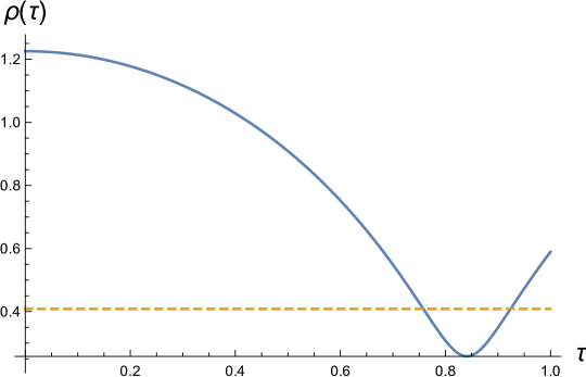
A solution beginning with a total energy will collapse and will oscillate about the local minimum of , provided that (in the case of attractive self-interactions).
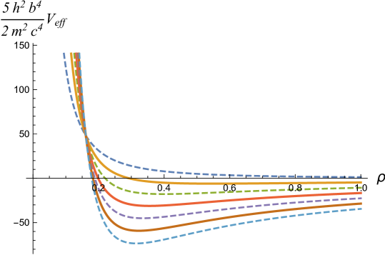
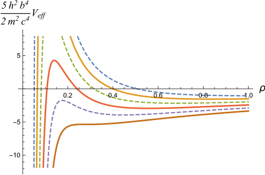
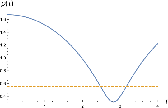
BEC clouds with repulsive self-interactions always admit a global minimum of the energy functional. This is because the repulsive interactions in combination with the quantum pressure ensures that the potential energy grows without bound as (see figure (5)). There is therefore no limit to the size of the condensate apart from the requirement that the equilibrium radius is larger than the Schwarzschild radius. However, if we consider a halo of mass kg made of condensed bosons of mass energy ev and , we find and (). Figure (5) represents a numerical integration of (139) with these conditions if the halo is assumed to begin with zero initial velocity at , and shows the collapse rebounce and subsequent oscillation of the cloud about equilibrium. The cloud collapses in or approximately 2.5 by.
We have seen that there is no local minimum with a positive for clouds with attractive self interactions unless the number of bosons is below some critical value, , which is determined by the strength of the interactions. One can understand this as saying that beyond the attractive inter-particle energy is sufficient to overcome the quantum pressure and the condensate implodes. When a local minimum exists, the equilibrium radius, depends on the actual number of bosons, , present (see figure 7). The equilibrium energy, and also depends on the number of bosons. For an example, we have taken and (, ) and integrated (139) to obtain a snapshot of the collapse process beginning at with (see figure 7). As is to be expected because of the negative pressure and weakend gravitational field, the collapse of the halo is extremely slow, taking on the order of 10 by to cross equilibrium.
The first integral of the motion (150) allows us to determine the frequency of small oscillations about equilibrium. They occur with characteristic period
| (157) |
This gives approximately 1.3 by for repulsive self interactions with the above parameters and roughly four times longer for attractive self interactions. This discrepancy is to be expected as the contribution to the BEC pressure from repulsive interactions strengthens the gravitational attraction and weakens it when the interactions are negative.
V Summary
While the standard CDM paradigm for DM does well on very large scales, few of its predictions on scales less that 50 kpc have been successful. Chief among these are the absence of DM cusps at the centers of galaxies and the absence of an abundance of low mass and massive sub-halos predicted by the model. It is therefore worthwhile to analyze alternative models that behave like CDM on large scales but are more in keeping with observations on smaller scales. One such model proposes that at least a component of DM may consist of ultralight condensed bosons.
We have analyzed a model for gravitationally bound BEC dark matter vortices based on the Gross-Pitaevskii equation with quartic interactions, taking into account the effects of rotation. To include rotation, we introduced an axisymmetric background differing only weakly from flat space. By analyzing the weak field Einstein equations in the harmonic gauge, we determined the form of the metric and set up the non-relativistic action for the combined matter and gravitational fields. From this action we determined the equations governing the system and analyzed the criteria for stability.
In order to get a better feeling for stable configurations of the BEC, we used the variational approach. With a standard Gaussian Vortex ansatz for the trial wave function, in which the BEC halo is assumed to have a radial dependence of , we obtained estimates for small and large condensates. The number of bosons in the condensate and its size depend only on the mass of the bosons and the strength of the self-interactions. As in the case of non-rotating BECs, two distinct cases arise with the votex ansatz as well. When the self interactions are attractive, a local minimum of the effective potential energy is present only when the number of bosons in the cloud is below a certain critical value. There is also a local maximum of the effective potential energy. If the number of particles exceeds the upper limit or when the total energy is greater than the maximum of the potential energy, it appears that the cloud would collapse into a black hole. However, one cannot be sure of this outcome due to the non-relativistic, linear approximation used in this paper. Harko h14 , Levkov et. al. lpt17 and Eby et. al. emw17 have proposed, in an alternative scenario, that as the central density grows and exceeds a certain critical value a fraction of the bosons will get expelled from the condensate, which will then stabilize. When the interaction strength is large enough, we obtained a simple relation between the critical (maximum) mass and the critical (minimum) radius of the cloud on the one hand and the mass and the coupling strength of the bosons on the other. Even in the non relativistic limit examined here, no such upper limit on the number of bosons (except the Schwarzschild limit) is apparent when the self interactions are repulsive. In this case, there is always a global minimum of the effective potential energy.
For example we considered attractive interactions, inputting the values of the interaction strength, and mass, ev, for the QCD axion. We obtained stable condensates approximately 400 km in radius having a mass of approximately kg. On the other hand, for sufficiently light bosons it is possible to achieve BECs of galactic size. We found that taking the boson mass ev along with an interaction strength of yielded a cloud with an outer radius (the radius within which 99% of the matter is contained) of roughly 50 kpc. Because of the density profile of a vortex, the gravitational field due to the BEC inside the core is outward directed up to a distance of about 17% of the outer radius. In this example, the central region is roughly 6-8 kpc in radius and dominated by ordinary (baryonic) matter, with the BEC taking over the gross gravitational dynamics beyond this distance.
We also analyzed the dynamics of rotating BECs by considering time dependent wave functions. The time dependence was introduced by employing a collective coordinate description in terms of the condensate radius, . Equations for the evolution of were obtained from an effective action, achieved by integrating the action for the combined BEC and gravitational field. The choice of the trial wave function is not unique of course and the extent to which the results obtained with different trial wave functions differ qualitatively from one another is a topic for future investigation. In our ansatz there is just one free parameter and the system is one dimensional. The Poisson equations can be solved exactly and the gravitational potentials of the halo can be evaluated in analytical form. The motion of the condensate then becomes analogous to the motion of a single particle of variable mass in an effective potential. In an ansatz with multiple parameters one may expect multiple coupled equations, which could be considerably more difficult to solve. We showed from the dynamics that the equilibrium conditions are identical to the ones obtained earlier in the static case. Moreover, in both the attractive and repulsive cases, collapse from a diffuse state into the equilibrium state is a process that takes billions of years. We have also examined the time scale for small oscillations about equilibrium and found it to be, not surprisingly, on the same order of magnitude.
There are several aspects of this description that have not been addressed in this work. For one, our model does not include a microscopic mechanism for varying the number of particles in the condensate, so we cannot say what happens, for example, if a BEC near its critical mass is immersed in a cloud of free bosons. Again, our model does not include damping, so a BEC will oscillate about its equilibrium radius essentially forever. We will consider damped BEC models in a future work. It would also be interesting to examine what happens when several types of BECs or even a single boson with multiple accessible states share a single gravitational well.
Acknowledgments
L. C. R. W. thanks J. Eby, M. Leembruggen, M. Ma and P. Suranyi for discussions.
References
- (1) A. G. Riess et al., Astron. J. 116 (1998) 1009.
- (2) S. Perlmutter et al., Astrophys. J. 517 (2) (1999) 565.
- (3) D. J. Eisenstein et al, Astrophys. J. 633 (2005) 560.
- (4) E. Komatsu et. al., Astrophys. J. Suppl., 192 (2011) 18.
- (5) G. Hinshaw et. al., Astrophys. J. Suppl., 208 (2013) 19.
- (6) P.A.R. Ade et. al. (Planck), “Planck 2015 results. XIII. Cosmological parameters,” (2015), [arXiv:1502.01589].
- (7) A. G. Sanchez et. al., MNRAS 425 (2012) 415.
- (8) L. Anderson et. al., MNRAS 427 (2012) 3435.
- (9) M. G. Walker et. al., Astrophys. J., 704 (2009) 1274.
- (10) A. Vikhlinin et. al., Astrophys. J., 692 (2009) 1033.
- (11) A. B. Newman et. al., Astrophys. J., 765 (2013) 24.
- (12) J. Dubinski and R. G. Carlberg, Astrophys. J., 378 (1991) 496.
- (13) R. A. Flores and J. R. Primack, Astropys. J., 427 (1994) L1.
- (14) B. Moore, Nature 370 (1994) 629.
- (15) J. F. Navarro, C. S. Frenk, and S.D.M. White, Astrophysical J., 490 (1997) 493.
- (16) G. Gentile, C. Tonini and P. Salucci, Astron. Astrophys. 467 (2007) 925.
- (17) S.-H. Oh, W. J. G. de Blok, F. Walter, E. Brinks and R. C. J. Kennicutt, Astron. J. 136 (2008) 2761.
- (18) F. Donato, G. Gentile, P. Salucci, C. Frigerio Martins, M. I. Wilkinson, G. Gilmore, E. K. Grebel, A. Koch, R. Wyse, MNRAS 397 (2009) 1169.
- (19) F. Nesti and P. Salucci, JCAP 7 (2013) 16.
- (20) A. Klypin, A. V. Kravtsov, O Valenzuela and F. Prada, Astrophysical J., 522 (1999) 82.
- (21) B. Moore et. al. Astrophys. J. 524 (1999) L19.
- (22) V. Springel et. al., MNRAS 391 (2008) 1685.
- (23) M. Boylan-Kolchin et. al. MNRAS 398 (2009) 1150.
- (24) M. Boylan-Kolchin, J. S. Bullock, M. Kaplinghat, MNRAS 415 (2011) L40.
- (25) C. S. Frenk, S. D. M. White, Annalen der Physik 524 (2012) 507.
- (26) D. H. Weinberg, J. S. Bullock, F. Governato, R. Kuzio de Naray, and A.H.G. Peter, Proceedings of the National Academy of Science, 112 (2015) 12249.
- (27) J. Kormendy, N. Drory, R. Bender and M. E. Cornell, Astrophys. J. 723 (2010) 54.
- (28) F. Governato et. al., Nature 463 (2010) 203.
- (29) J. S. Bullock and M. Boylan-Kolchin, Ann. Rev. Astron. Astrophys. 55 (2017) 343.
- (30) D.J. Kaup, Phys. Rev. 172 (1968) 1331.
- (31) R. Ruffini, S. Bonazzola, Phys. Rev. 187 (1969) 1767.
- (32) W. Thirring, Phys. Lett. B 127 (1983) 27.
- (33) G. Ingrosso, M. Merafina, R. Ruffini, Nuovo Cimento 105 (1990) 977.
- (34) C. G. Boehmer and T. Harko, JCAP 0706 (2007) 025.
- (35) J. D. Breit, S. Gupta, A. Zaks, Phys. Lett. B 140 (1984) 329.
- (36) M. S. Turner, Phys. Rev. D 28 (1983) 1243.
- (37) W. H. Press, B. S. Ryden, and D. N. Spergel, Phys. Rev. Lett., 64 (1990) 1084.
- (38) S.-J. Sin, Phys. Rev. D 50 (1994) 3650.
- (39) W. Hu, R. Barkana, and A. Gruzinov, Phys. Rev. Lett., 85 (2000) 1158.
- (40) J. Goodman, New Astron. 5 (2000) 103.
- (41) P.J.E. Peebles, Astrophys. J. 534 (2000) L127.
- (42) L. Amendola and R. Barbieri, Phys. Lett., B 642 (2006) 192.
- (43) P-H Chavanis, Phys. Rev. D 84 (2011) 043531.
- (44) H.-Y. Schive, T. Chiueh, and T. Broadhurst, Nature Phys. 10 (2014) 496.
- (45) T. Rindler-Daller, P. R. Shapiro, Mod. Phys. Lett. A 29 (2014) 1430002.
- (46) B. Li, T. Rindler-Daller, P. R. Shapiro, Phys. Rev. D 89 (2014) 083536.
- (47) L. Hui, J. P. Ostriker, S. Tremaine, E. Witten, Phys.Rev. D 95 (2017) 043541.
- (48) P. Horava, E. Witten, Nucl. Phys. B 460 (1996) 506.
- (49) U Günther, A. Zhuk, Phys. Rev. D 56 (1997) 6391.
- (50) N. Arkani-Hamed, S. Dimopoulos, G. Dvali, Phys. Rev. D 59 (1999) 086004.
- (51) A. Arvanitaki, S. Dimopoulos, S. Dubovsky, N. Kaloper, J. March-Russell, Phys. Rev. D 81 (2010) 123530.
- (52) M. Colpi, S. L. Shapiro, I. Wasserman, Phys. Rev. Lett. 57 (1986) 2485.
- (53) M. Yu. Khlopov, B. A. Malomed and Ya. B. Zeldovich, Mon. Not. Roy. Astr. Soc., 215 (1985) 575.
- (54) Z. G. Berezhiani, A. S. Sakharov, and M. Yu. Khlopov, Sov. J. Nucl. Phys. 55 (1992) 1063.
- (55) A. S. Sakharov and M. Yu. Khlopov, Phys. Atom. Nucl. 57 (1994) 485.
- (56) A. S. Sakharov, D. D. Sokoloff, and M. Yu. Khlopov, Phys. Atom. Nucl. 59 (1996) 1005.
- (57) M. Yu. Khlopov, A. S. Sakharov, and D. D. Sokoloff, Nucl.Phys. B (Proc. Suppl.) 72 (1999) 105.
- (58) S. G. Rubin, A. S. Sakharov, M. Yu. Khlopov, J. Exp. Theor. Phys. 92 (2001) 921.
- (59) M. Yu. Khlopov, S. G. Rubin, A. S. Sakharov, Astropart. Phys. 23 N-2 (2005) 265.
- (60) M. Yu. Khlopov, Res. Astron. Astrophys. 10 (2010) 495.
- (61) J. Barranco and A. Bernal, Phys. Rev. D 83 (2011) 043525.
- (62) A. H. Guth, M. P. Hertzberg, C. Prescod-Weinstein, Phys.Rev. D 92 (2015) 103513.
- (63) J. Eby, P. Suranyi, C. Vaz and L.C.R. Wijewardhana, JHEP (2015) 2015: 80.
- (64) J. Eby, M. Leembruggen, P. Suranyi and L.C.R. Wijewardhana, JHEP (2016) 2016: 66.
- (65) D. G. Levkov, A. G. Panin and I. I. Tkachev, Phys. Rev. Lett. 118 (2017) 011301.
- (66) P-H Chavanis, “Phase Transitions between Dilute and Dense Axions”, [arXiv:1710.06268].
- (67) T. Helfer, D. J. E. Marsh, K. Clough, M. Fairbairn, E. A. Lim, R, Becerril, JCAP 1703(03) (2017) 055.
- (68) E. D. Schiappacasse, M. P. Hertzberg, [arXiv:1710.04729].
- (69) V. Silveira, C. M. G. de Sousa, Phys. Rev. D 52 (1995) 5724.
- (70) M. R. Matthews et. al., Phys. Rev. Lett. 83 (1999) 2498.
- (71) T. Rindler-Daller and P. R. Shapiro, MNRAS, 422 (1)(2012) 135.
- (72) S. Davidson, T. Schwetz, Phys. Rev. D 93 (2016) 123509.
- (73) For example, C. J. Pethick and H. Smith, “Bose-Einstein Condensation in Dilute Gases”, Cambridge University Press, 2008.
- (74) M. Bijlsma and H.T.C. Stoof, Phys.Rev. A55 (1997) 498.
- (75) For example, T. Padmanabhan, “Gravitation: Foundations and Frontiers”, Cambridge University Press, 2014.
- (76) A. Suárez and Pierre-Henri Chavanis, J. Phys: Conf. Series 654 (2015) 012008.
- (77) R. Arnowitt, S. Deser and C.W. Misner in “Gravitation: An Introduction to Current Research”, ed. Louis Witten, Wiley, New York (1962).
- (78) E. Madelung, Z. Phys. 40 (1927) 322.
- (79) P-H Chavanis, “Dissipative self-gravitating Bose-Einstein condensates with arbitrary nonlinearity as a model of dark matter halos”, [arXiv:1611.09610].
- (80) H. T. C. Stoof, J. Stat. Phys. 87 (1997) 1353.
- (81) J. A. Freire and D. P. Arovas, Phys. Rev. A 59 (1999) 1461.
- (82) P-H Chavanis and L. Delfini, Phys. Rev. D 84 (2011) 043532.
- (83) J. Eby, C. Kouvaris, N. Grønlund Nielsen, L.C.R. Wijewardhana, JHEP (2016) 2016: 28.
- (84) E. Casuso and J. E. Beckman, Mon. Not. R. Astron. Soc. 000 (2015) 1.
- (85) F. Iocco, M. Pato and G. Bertone, Phys. Rev. D 92 (2015) 084046.
- (86) M. Pato and F. Iocco, Astrophys. J. 803 (2015) L3.
- (87) F. Iocco, M. Pato and G. Bertone, Nature Phys. 11 (2015) 245.
- (88) M. Ueda and A. J. Leggett, Phys. Rev. Lett. 80 (1998) 1576.
- (89) T. Harko, Phys. Rev. D 89 (2014) 084040.
- (90) J. Eby, M. Ma, P. Suranyi, L.C.R. Wijewardhana, JHEP 1801 (2018) 066.