Gravitons and Temperature Fluctuation Correlations from Inflation
Abstract
Inflationary tensor perturbations are treated as arising from a bath of gravitons produced by quantum particle creation at the end of inflation. We calculate the correlation function of the CMB temperature fluctuations produced by these gravitons in a model with an infrared cut off. The CMB photons are emitted from within a last scattering shell of finite thickness in redshift. We find the correlation function in terms of the separation of a pair of spacetime points of emission in both angle and redshift. In both variables, there is a significant amount of anti-correlation. The anti-correlation minimum has a relative magnitude compared to the central correlation maximum of about in angle and in redshift.
I Introduction
This work will re-examine inflationary tensor perturbations from a viewpoint which emphasizes their quantum origin and nature. Starobinsky S79 was apparently the first author to suggest that a period of deSitter expansion could produce an observable spectrum of gravity wave perturbations in the subsequent universe. This early work was soon followed by contributions from several authors, including Rubakov, Sazhin, and Veryaskin RSV82 , Fabbri and Pollack FP83 , Abbott and Wise AW84b , Abbott and Harari AH86 , Polnarev Polnanev , and Allen A88 .
A key result found in Refs. FP83 ; Polnanev is that a classical gravitational wave propagating in an expanding universe induces an anisotropic pattern of redshifts on photons also propagating in this universe. These are the tensor perturbations in the Cosmic Microwave Background (CMB) which may be observable. When these anisotropically redshifted photons scatter from electrons, a particular polarization pattern (the B-modes) is induced and may serve as an observational signal of primordial gravity waves. For a review, see Kamionkowski and Kovetz KK16 .
Inflation does not produce a single mode gravitational wave, but rather a spectrum of wave numbers and polarization states. This mixture is often described as a stochastic bath of gravity waves. However, a deeper approach involves quantum creation of gravitons by the expansion of the universe, a process first described by Parker Parker69 and applied to graviton creation in Refs. Grishchuk:1975 ; FordParker:1977 . For a review, see Ref. pp-review . Calculations of graviton creation at the end of inflation were given by Abbott and Harari AH86 and by Allen A88 . The quantum state of the created gravitons is predicted to be highly nonclassical, specifically a squeezed vacuum state GS89 .There has been an extensive discussion in the literature as to whether there is a quantum to classical transition and to whether the gravitons undergo decoherence PS96 ; GS19 ; Kanno22 ; Burgess23 ; Ning23 .
In the present paper, we explore the hypothesis that no quantum to classical transition occurs, and the gravitons remain in a nonclassical state when they interact with the CMB photons. The outline of the paper is the following: In Sect. II we review quantum graviton creation at the end of inflation, and discuss the resulting quantum state in Sect. III. The effects of the gravitons on the CMB photons is treated in Sect. IV. Section V contains our main results on the temperature correlation function and its physical implications. Section VI gives a summary.
II Graviton creation at the end of inflation
This section will review the basic principles of quantum particle creation in an expanding universe and application to inflationary cosmology.
II.1 Gravitons in a Spatially Flat Universe
Here we consider the spatially flat Friedman-Robertson-Walker spacetime with metric
| (1) |
where and are the comoving and conformal time coordinates, respectively. We are interested in treating gravitons propagating on this background spacetime. It was shown by LifshitzLifshitz that in the transverse, tracefree gauge, which eliminates all gauge freedom, each of the two independent polarization states is equivalent to a massless, minimally coupled scalar field which satisfies
| (2) |
The positive norm plane wave solutions of this equation may be taken to be
| (3) |
where is the Planck length and we use the normalization for graviton modes, which is a factor of times that for the scalar field, Here satisfies
| (4) |
where is the scalar curvature.
First consider the spacetime of the inflationary model, deSitter space, where we may take
| (5) |
where is the Hubble parameter and . Here denotes the time when inflation began and that when it ends in reheating. Here the scalar curvature is . The solutions of Eq. (4) may be expressed in terms of Hankel functions as
| (6) |
where
If we set and , the resulting mode function
| (7) |
defines the Bunch-Davies vacuum state of deSitter space BD78 . In the case of a massive scalar field, it is the unique deSitter invariant state, and is analogous to the Minkowski vacuum, the unique Lorentz invariant state in flat spacetime. However, the massless scalar field has a infrared divergent two-point function, , so the Bunch-Davies state is not well defined for either the massless scalar or the graviton fields. There is a class of states which are free of infrared divergences FordParker:1977b ; FV86 . If we require that as , then the two-point function is infrared finite. This class may be said to be Bunch-Davies-like if we also have and for for some small cutoff scale . We can view this scale as set by some initial condition before the onset of inflation. If is sufficiently small that the associated modes have not entered the horizon since the end of inflation, then they seem to play no role in present cosmological observations. In this case, we may take Eq. (7) as the initial graviton mode before reheating.
II.2 The transition from Inflation to a Radiation Dominated Universe
The creation of gravitons at the end of inflation may be viewed as gravitational particle creation described by a Bogolubov transformation. Here we take the in-modes to be the Bunch-Davies-like modes given by Eqs. (3) and (7). In the subsequent radiation dominated phase, the scalar curvature vanishes, , so the positive unit norm mode functions become
| (8) |
We are interested in very long wavelength gravitons modes which are far outside the horizon at the end of inflation, so . These modes are not sensitive to the finite duration of reheating, so we assume a sharp transition in which the scale factor is given by Eq. (5) for and by
| (9) |
for . Note that we take the reheating time to be and have set .
The mode functions in the in and out regions are related by a Bogolubov transformation of the form
| (10) |
where
| (11) |
The Bogolubov coefficients may be found by using Eq. (10) and its first time derivative at , using the fact that both and are continuous at this point. The results AH86 ; A88 are
| (12) |
and
| (13) |
The mean number of gravitons created in a given mode is . Here that number is very large. The energy spectrum of created gravitons is scale invariant in the sense that the graviton energy density in wave number interval is proportional to , which independent of the choice of scale for . Note that in a spatially flat expanding universe, linear three-momentum is conserved, so the gravitons are created in pairs with equal and opposite wave vectors, and
III The Quantum State of the Created Gravitons
III.1 Representation in the Out-Fock Space
The quantum particle creation process is being described in the Heisenberg picture, so the quantum state of the system, , does not change in time. However, its description is very different in the deSitter space in-region from that in the radiation dominated out-region. In the in-region, it is one of several infrared finite choices of vacuum state. In the out-region, it is a highly excited state with very large numbers of particles in modes for which .
The quantum state of the created particles in the out-Fock space may be shown to be
| (14) |
where . Here denote a set of occupation numbers; for each mode there is non-negative integer which gives the number of particles in mode and the number of particles in mode . In our enumeration, we may require to avoid over counting. The overall constant satisfies
| (15) |
where the latter form follows from Eq. (11). This quantum state is a multi-mode squeezed vacuum state, containing all possible numbers of pairs of correlated particles. Strictly, Eq. (14) applies to the massless scalar field. For gravitons, we need to include the polarization among the mode labels. This will be explicitly addressed in Sect IV.1, where a sum over polarizations will be performed.
In the single mode case, only one type of pair is present. Here we have
| (16) |
where denotes a state containing pairs, with one member of the pair in mode , and the other in mode .
III.2 The Observable Part of the State
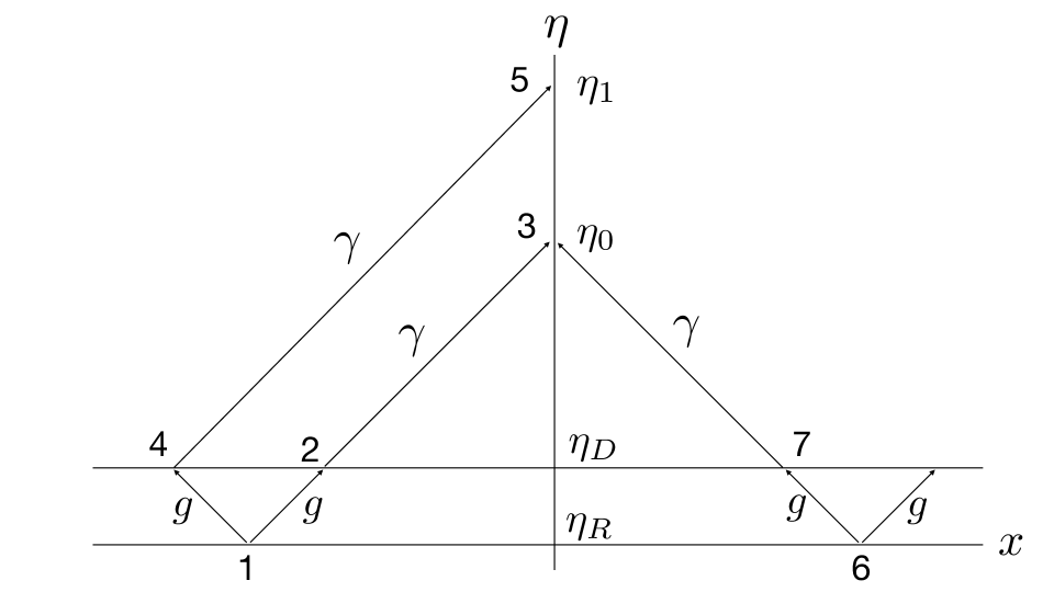
It is well known in quantum theory that outcomes of observations can depend crucially upon the details of the question which is addressed, or the specific measurement which is undertaken. At least in the cosmological case, we can only observe one member of a pair of correlated gravitons. This can be seen if we adopt a set of wave packet mode functions, rather than plane waves with a precisely defined wave vector. Consider a set of wave packets with a finite but small bandwidth, , where is the peak wave vector of a packet. These packets will have a spatial extent of order .
In the wave packet basis, the correlated pairs of gravitons are created into a pair of packets peaked about values of with equal magnitude, but opposite sign. This means that the two packets leave the region of their creation in opposite directions. A given observer will be able to observe at most one of these gravitons. This is illustrated in Fig, 1 for the case of gravitons which influence the redshifts of CMB photons.
Suppose we are making measurements of local field operators in a spacetime region , and using a complete set of wave packets with mode labels . It is convenient to divide the set into two subsets, and , where the modes are nonzero in , and the modes vanish there and do not contribute to local expectation values in . Now we can rewrite Eq. (14) as
| (18) |
Equation (16) is the special case where there is one mode and one mode.
If and are two modes in set , then the expectation values in state of the associated creation and annihilation operators are
| (19) |
but
| (20) |
This implies that expectation values of linear field operators vanish in this state, but those of quadratic operators can be nonzero. Furthermore, the effects of the state in are equivalent to a density matrix.
Let and be associated with any given mode in set , and define a coordinate by
| (21) |
and a conjugate momentum by
| (22) |
Then , but the ubcertainties are nonzero: . Furthermore the uncertainty relation becomes
| (23) |
In general, is not a state of minimum uncertainty, unlike the Stoller squeezed states, and will have very large uncertainty when . This implies large fluctuations, as evidenced the large variance of linear field operators.
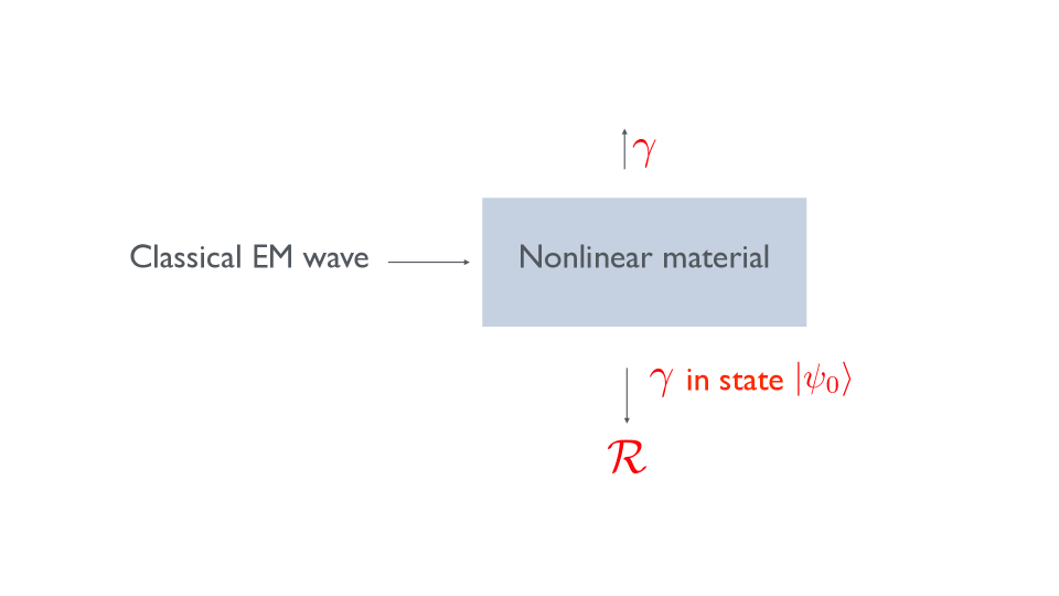
III.3 An Electromagnetic Analog Model
There is a simple analog involving a squeezed state of photons which is illustrated in Fig. 2. A strong classical electromagnetic wave in a nonlinear material with a nonzero second or third order susceptibility creates a time dependent effective index of refraction for vacuum electromagnetic modes. This leads to mixing of positive and negative frequencies and quantum creation of photons, an effect analogous to the quantum creation of gravitons in inflation discussed in Sect. II. The photons are emitted in correlated pairs in opposite directions from the material in a quantum state of the form of given in Eq. (18).
III.4 Scalar Correlation Functions
In this subsection, we focus on the case of a single massless, minimally coupled scalar field , which is equivalent to one polarization state of the graviton field in the transverse tracefree gauge. Assume that we are in the radiation dominated era, when the mode functions may be given by Eq. (8) and the field operator may be expressed as
| (24) |
where the satisfy the relations in Eqs. (19) and (20) in a state of the form of . Next define a correlation operator by
| (25) |
and a correlation function by
| (26) |
Recall that , so is the variance of the fluctuations of . If , then
| (27) |
where we ignore a term of order .
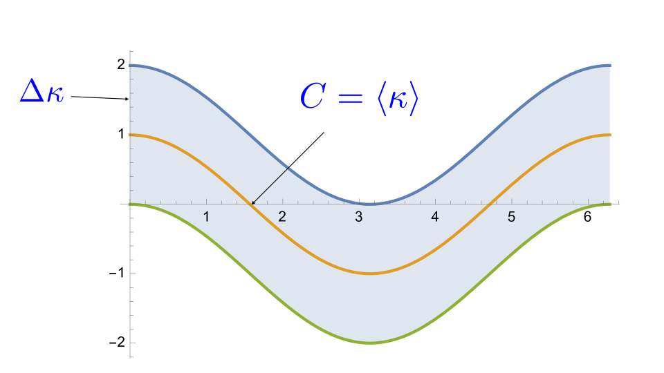
Consider the case where a single mode gives the dominant contribution to , so that , and the correlation function has the form of a classical wave as a function of for fixed . This is similar to the case of a coherent state. However, unlike a highly excited coherent state, here the fluctuations of the correlation operator are very large:
| (28) |
so the fractional variance of is of order one
| (29) |
The fluctuations are illustrated in Fig. 3. Because of the large fractional fluctuations, the correlation effects can only be observed in an ensemble average.
IV Effects of Gravity Waves and of Gravitons on CMB Photons
IV.1 Differential Redshifts due to a Classical Gravity Wave
IV.1.1 Polarization
The metric may be written as
| (30) |
where . The equation for the four-velocity of a timelike geodesic is
| (31) |
where is the observer’s proper time, and . The connection coefficient which we need is, to first order in ,
| (32) |
Hence the geodesic equation has the solution . This tells us that the comoving observers are at rest in the coordinates of Eq. (30). Let be the 4-dimensional wave vector of a photon. The angular frequency of this photon in the comoving observer’s frame is
| (33) |
We may find the wave vector either from geodesic equation, or the null vector condition, . Here we use the latter. In the metric of Eq. (30) we find
| (34) |
In the isotropic case where , we have , where
| (35) |
Here and are the direction angles for the photon in a frame where the gravity wave propagates in the -direction, and is the photon angular frequency when The factor of arises because and is an affine parameter. The latter may be taken to be given by . (See, for example, Visser23 .)
To first order in , we may place the above expressions for the zero order spatial components in the right hand side of Eq. (34), Taylor expand, and use Eq. (33) to find
| (36) |
The pre-factor, , is the redshifted frequency in an isotropic universe, and the term proportional to gives the fractional anisotropic redshift due to the gravity wave. Specifically, we define the fractional redshift by
| (37) |
Apart from a sign difference, this agrees with the result of Polnarev Polnanev which is quoted in Ref. KK16
IV.1.2 Polarization
Now the metric may be written as
| (38) |
where . If we repeat the procedure in the previous subsection, the result is
| (39) |
Note that if we let , then , as a rotation by interchanges the two polarizations. Now the fractional redshift becomes
| (40) |
Note that if , then
| (41) |
Thus the dependence upon the angle disappears from a sum over polarization states.
IV.2 The Quantized Graviton Field
The graviton field operator may be expanded in terms of mode functions as
| (42) |
where is the polarization tensor for mode . The expectation value of in a coherent state for mode is a classical gravitational wave. Here we use a linear polarization basis, so , and the polarization tensors are implicitly defined by Eqs. (30) and (38).
V The Temperature Correlation Function
The graviton correlation function, Eq. (43) may be used to compute a CMB temperature fluctuation correlation function using the results of Sect. IV.1. Equation (41) was derived for classical gravity waves, but also applies expectation values in a graviton bath if we replace by an expectation value of a quadratic graviton operator. Specifically, we can convert Eq. (43) into a result for the fractional temperature fluctuation correlation function:
| (44) |
where , and we are interested in the correlation between photons emitted at spacetime point with those emitted at . Here denotes the angle between our line of sight and the graviton wave vector . We have used Eq. (41) to make the replacement .
V.1 The infrared Cutoff
If we use Eq. (13), with , then the integral in Eq. (44) will diverge at the lower limit. This issue is most likely distinct from the infrared divergence discussed in Sect. II.1 which required a cutoff at . The latter was required because gravitons and massless minimally coupled scalar fields necessarily break deSitter symmetry. The cutoff at arises from a memory of pre-inflationary conditions which is was not erased by a finite amount of inflation. The infrared divergence carried by is most likely due to a breakdown of the particle interpretation of the out-Fock space. Recall that is interpreted as the mean number of gravitons in mode in the out-region. However, it is not clear that graviton number is meaningful for modes whose wavelength is far greater than the horizon size. We propose to modify Eq. (44) by restricting the integration to modes with , where is the wave number associated with the horizon size at the time when the gravitons interact with the CMB photons. Thus, Eq. (44) is replaced by
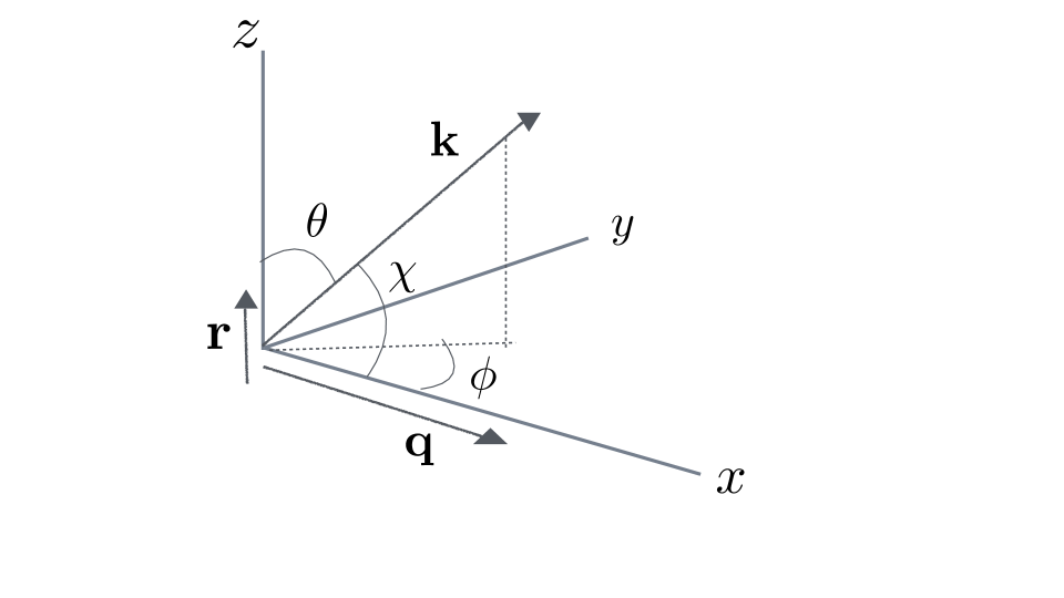
| (45) |
The angles involved in the integration are illustrated in Fig. 4. First note that . Thus , with and we have
| (46) |
Now we can write
| (47) |
where we define a reduced correlation function by
| (48) |
which is normalized by . The reduced correlation function may be expressed in terms of the functions and are defined by
| (49) |
and
| (50) |
These functions may be expressed in terms of trigonometric and cosine-integral functions and are given in the Appendix.
V.2 Results: Case
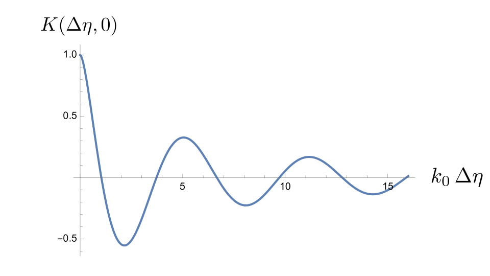
In this subsection, we deal with the simpler case where , but is nonzero. This is the case where the CMB photons arrive from the same direction, but were emitted at different times and hence different redshifts. In this case there is no angle dependence inside the cosine function in Eq. (48), and we find
| (51) |
which is plotted in Fig. 5. This function describes the temperature fluctuations correlations for photons arriving from the same direction, but different redshifts, with the pre-factor of in Eq. (45) removed.
Note that the region in which the inflationary gravitons interact with the CMB photons is actually a last scattering shell of finite thickness. This thickness is determined by the time required for the electrons and protons in the primordial plasma to combine into neutral hydrogen atoms. It has been estimated by Hadzhiyska and Spergel HS19 to be of order , which is equivalent to in redshift.
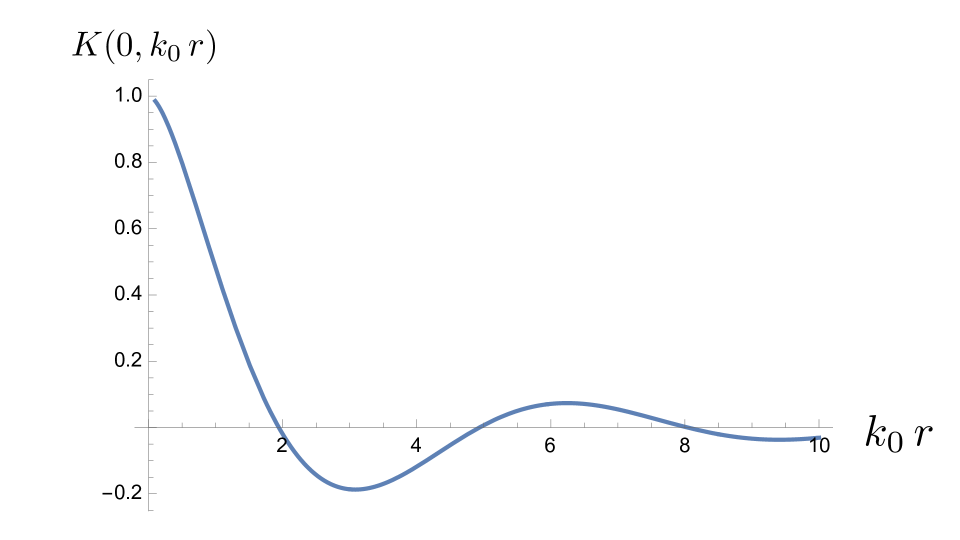
V.3 Results: Case
When , the argument of the cosine function in Eq. (45) depends upon . In this case, we have
| (52) |
We may now write Eq. (48) as
| (53) | |||||
with and .
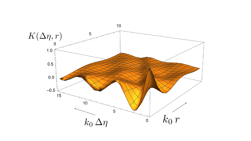
The case of spatial separation alone, is plotted in Fig. 6, and the general case is illustrated in Fig. 7.
V.4 Physical Meaning of the Correlations
We have seen in the previous subsection that the temperature fluctuations produced by a graviton bath display distinctive correlations and anti-correlations, both in space and in time. The anti-correlations mean that a region whose temperature is above average, is more likely to be near a region which is cooler than average, and vice versa. The separation between the hotter and the cooler region can be either in angle or in redshift. The magnitude of the expected angular or redshift depends upon the unknown parameter , and is given by for spatial or angular separations and by for temporal or redshift separations. Note that the ratio of these two expected separations, , is independent of . As was emphasized in Sec. III.4 and illustrated in Fig. 3, correlation functions are averages of highly fluctuating quantities. This means that the temperature anti-correlations can only be observed by averaging over several pairs of regions.
VI Summary
We have presented a description of inflationary tensor perturbations in terms of gravitons created by quantum particle creation at the end of inflation. These gravitons are in a multi-mode squeezed vacuum state describing pairs of created gravitons. However, only one member of each pair is observable, and the resulting quantum state exhibits large fluctuations and is equivalent to a density matrix . Our description introduces two infrared cutoffs. The first is the parameter introduced in Sect. II.1, and depends upon initial conditions before the onset of inflation. This parameter is expected to be very small and its effects to be unobservable. The second cutoff is the parameter introduced in Sect. V.1, and determined by the range of validity of the concept of graviton number in the out-region. It is an undetermined in our analysis, but is expected to be determined by the horizon size at the time of last scattering. We have followed the approach of previous authors, and calculated the CMB temperature anisotropies from solutions of the photon geodesic equations. This leads to the temperature fluctuation correlation function in terms of the graviton correlation function, Eq. (43). The cutoff is used to make these expressions infrared finite.
An alternative approach may be to use the geodesic deviation equation to study the perturbations of the photon geodesics. This would replace the correlation function for the graviton field by that for the associated Riemann tensor. The letter contains additional derivatives which are expected to render it infrared finite. This approach will be the topic for future research.
Within our present approach, we are able to obtain an explicit expression, Eq. (53), as a function of the temporal separation and spatial separation of a pair of emission points. Recall that is equivalent to an angular separation on the sky, and is equivalent to a redshift separtion within the last scattering shell. The plots of this function in Figs. 5, 6, and 7, reveal significant anti-correlations in both angle and redshift. This means that a hot region will tend to be associated with a nearby cooler region, and vice versa. As was emphasized in Sect. III.4, these anti-correlations will appear only in averages over many pairs of emission points. However, if the anti-correlations can be observed, it will provide strong evidence for the existence of inflationary gravitons.
Acknowledgements.
We would like to thank J.T. Hsiang, B.L. Hu, and K.W. Ng for helpful discussions. LHF would like to thank the Department of Physics, Soochow University for hospitality while part of this work was performed. This work was supported in part by the National Science Foundation under Grant PHY-2114024.Appendix A Integrals Appearing in the Correlation Functions
Here we give the explicit forms for some of the integrals which appear in the correlation function, Eq. (53). For odd, , defined in Eq. (49), is given by (See Formula 3.761.8 in Ref, GR .)
| (54) |
where is the cosine integral function. The special cases of interest to us are the following:
| (55) |
| (56) |
and
| (57) |
References
- (1) A.A. Starobinsky, Spectrum of relict gravitational waves and the early universe, Pis’ma Zh. Teor. Fiz. 30, 719-723 (1979) [JETP Lett. 30, 682-685 (1979)].
- (2) V.A. Rubakov, M.V. Sazhin, and A.V. Veryaskin, Graviton creation in the inflationary universe and the grand unification scale, Phys. Lett. 115B, 189-192 (1982).
- (3) F. Fabbri and M.D. Pollack, The effect of primordially produced gravitons upon the anisotropy of the cosmological microwave background radiation, Phys. Lett. 125B, 445-448 (1983).
- (4) L.F. Abbott and M.B. Wise, Constraints on generalized inflationary cosmologies, Nucl. Phys. B244, 641-548 (1984).
- (5) L.F. Abbott and M.B. Wise, Anisotropy of the microwave background in the inflationary cosmology, Phys. Lett. 135B, 279-282 (1984).
- (6) L.F. Abbott and Harari, Graviton production in inflationary cosmology, Nucl. Phys. B264, 487-492 (1986).
- (7) A.G. Polnarev, Sov. Astron. 29, 607 (1986).
- (8) B. Allen, Stochastic gravity-wave background in inflationary-universe models, Phys. Rev. D 37, 2078-2085 (1988).
- (9) M. Kamionkowski and E.D. Kovetz, The Quest for B Modes from Inflationary Gravitational Waves, Annu. Rev, Aston. Astrophys. 54, 227-69 (2016).
- (10) L. Parker, Quantized fields and particle creation in expanding Universes. I, Phys. Rev. 183, 1057 (1969).
- (11) L. P. Grishchuk, Amplification of gravitational waves in an isotropic universe, Zh. Eksp. Teor. Fiz. 67, 825 (1974) [Sov. Phys. JETP 40, 409 (1975)].
- (12) L. H. Ford and L. Parker, Quantized gravitational wave perturbations in Robertson-Walker universes, Phys. Rev. D 16, 1601 (1977).
- (13) L.H. Ford, Cosmological Particle Production: A Review, Rep. Prog. Phys. 84, 116901 (2021) , arXiv:2112.02444.
- (14) L. P. Grishchuk and Y.V. Sidorov, On the quantum state of relic gravitons, Class. Quantum Grav. 6, L161 (1989).
- (15) D. Polarski and A. A. Starobinsky, Semiclassicality and decoherence of cosmological perturbations, Class. Quantum Grav. 13, 377 (1996)
- (16) J-O Gong and M-S Seo, Quantum non-linear evolution of inflationary tensor perturbations, JHEP 2019, 21 (2019), arXiv:1903.12295
- (17) S. Kanno, J. Soda and K. Ueda, Conversion of squeezed gravitons into photons during inflation, Phys. Rev. D 105, 083508 (2022), arXiv:2207.05734.
- (18) C. P. Burgess, R. Holman, G. Kaplanek, J.Martin, and V. Vennin, Minimal decoherence from inflation, JCAP 07 (2023) 022 [ arXiv:2211.11046 ]
- (19) S. Ning. C. M. Soub, and Y. Wangb, On the decoherence of primordial gravitons, JHEP06(2023)101
- (20) E. M. Lifshitz, On the Gravitational Stability of the Expanding Universe, Zh. Eksp. Teor. Fiz. 16, 587 (1946) [J. Phys. USSR 10, 116 (1946)].
- (21) T.S. Bunch and P.C.W. Davies, Quantum field theory in de Sitter space - Renormalization by point-splitting, Proc. Roy Soc. London 360, 117-134 (1978).
- (22) L. H. Ford and L. Parker, Infrared divergences in a class of Robertson-Walker universes, Phys. Rev. D 16, 245 (1977).
- (23) L.H. Ford and A. Vilenkin, Global Symmetry Breaking in Two-Dimensional Flat Spacetime and in de Sitter Spacetime, Phys. Rev. D 33, 2833-2839 (1986).
- (24) M. Visser, Efficient computation of null affine parameters , Universe 9, 521 (2023) [arXiv:2211.07835].
- (25) I. S. Gradshteyn and I. M. Ryzhik, Table of integrals, series, and products, 7th ed. Academic Press (2007).
- (26) B. Hadzhiyska and D. Spergel, Phys. Rev. D 99, 043537 (2019) [arXiv:1808.04083].