Gravity dualities of quantum distances

In recent years it has been suggested that quantum information theory and gravity theory have deep connection. The gauge/gravity duality, which shows an equivalence between strongly coupled quantum field theories (QFTs) and weakly coupled gravitational theories in one higher dimensions Maldacena:1997re ; Gubser:1998bc ; Witten:1998qj , offers us a powerful tool towards such connection. As a result, the quantum information theoretic considerations have provided various useful viewpoints in the studies of gauge/gravity duality and quantum gravity. One example is the Ryu-Takayanagi (RT) formula Ryu:2006bv ; Hubeny:2007xt ; Chen:2019lcd , which connects the area of a codimension-2 minimal surface in the dual spacetime and the entanglement entropy of the boundary QFT. The RT formula has been generalized into the Rényi entropy Hung:2011nu ; Dong:2016fnf , higher order gravity theory Dong:2013qoa ; Camps:2013zua ; Miao:2014nxa and the cases with quantum corrections Faulkner:2013ana ; Engelhardt:2014gca . An other quantity in quantum information named “complexity”, which measures the difference of two states according to the size of quantum circuits in converting one state into the other, also has been studied widely in gravity and black hole physics Harlow:2013tf ; Stanford:2014jda ; Susskind:2014rva ; Brown:2015bva ; Czech:2017ryf ; Caputa:2018kdj .

From a general viewpoint, the complexity is a kind of “distance” between quantum states Susskind:2014jwa . Except for complexity, there are other several different measures of the distance between states, which are widely used in quantum information Nielsen:2011:QCQ:1972505 ; Watrous . For example, given two density matrices $\rho$ and $\sigma$ in the same Hilbert space, two families of distance are widely used in quantum information theory. The first one are based on the fidelity

The fidelity is not a distance but we can use it to define two kinds of distance, the Fubini-Study distance $D_{F}(\rho,\sigma)=\arccos\text{Fi}(\rho,\sigma)$ and the Bures distance $D_{B}(\rho,\sigma)=\sqrt{1-\text{Fi}(\rho,\sigma)}$. The other family of distances, depending on a positive number $n$, is provided by the $n$-distances

Here ${\text{Tr}}|X|^{n}:=\sum_{i}\lambda_{i}^{n}$ and $\lambda_{i}$ is the $i$-th eigenvalue of $\sqrt{X^{\dagger}X}$. When $X$ is hermitian $\{\lambda_{i}\}$ are just the the absolute values of eigenvalues of $X$. Two special choices are widely applied. One is Hilbert-Schmidt distance, which chooses $n=2$. This distance leads to some conveniences in mathematics because the calculation is straightforward by its definition. The other choice is $n=1$, which is called the “trace distance”.

Though the trace distance and fidelity are complicated than Hilbert-Schmidt distance, several properties make them special Nielsen:2011:QCQ:1972505 . Firstly, the trace distance and fidelity (and so Fubini-Study distance and Bures distance) are bounded by each others: $1-D_{1}\leq\text{Fi}\leq\sqrt{1-D_{1}^{2}}$. Secondly, they offer us dimension-independent bounds on the difference between the expected values of an operator $O$ in different states: $|\langle O\rangle_{\rho}-\langle O\rangle_{\sigma}|\leq D_{1}(\rho,\sigma)\sqrt{{\text{Tr}}(OO^{\dagger})}\leq\sqrt{1-\text{Fi}(\rho,\sigma)^{2}}\sqrt{{\text{Tr}}(OO^{\dagger})}$. Thirdly, they supply lower bounds for the relative entropy $S(\rho\parallel\sigma)$: $[1-\text{Fi}(\rho,\sigma)]\leq D_{1}(\rho,\sigma)\leq\sqrt{S(\rho\parallel\sigma)/2}$.

Despite that trace distance and fidelity have these important properties, their computations are high challenge in quantum field theory. The first breakthrough towards this issue is achieved by Ref. PhysRevLett.113.051602 , which develops a replica trick to compute the fidelity for 2-dimensional conformal field theory. Refs. Zhang:2019wqo ; Zhang:2019itb ; Zhang:2019kwu then also develop replica method to compute the trace distance for a class of special states for single short interval in 1+1 dimensional CFTs. However, there are still huge difficulties in the calculations of trace distance even for 1+1 dimensional CFTs, such as to compute the trace distance between two thermal states or two large intervals in CFTs. There is also no compact method to compute the trace distance in higher dimensional CFTs or general quantum field theories. On the other hand, the holographic descriptions of entanglement, relative entropy Blanco:2013joa and complexity have been found, however, the trace distance does not yet. Refs. PhysRevLett.115.261602 ; PhysRevD.96.086004 propose holographic duality to compute the fidelity between a state and its infinitesimal perturbational state, however, they cannot be used into the case when the difference between two states are not infinitesimal.

In this paper, it will develop holographic dualities to compute the trace distance, Fubini-Study distance, Bures distance and Rényi relative entropy. By choosing a characteristic reference state which will be called “modular ground state”, they all become the intrinsic properties of the target state. Then this paper will show that they all have gravity dualities. Their gravity dualities have two equivalent descriptions. The one is given by the integration of the area of a cosmic brane with respective to its tansion. The other one description contains two parts, one of which is the on-shell action of gravity theory and the other one of which is the area of the cosmic brane. We then apply them to the calculations of the trace distance in 1+1 dimensional CFT and show our holographic calculations exactly match with the results of CFT’s.

In the field theory two different density matrices will often be almost orthogonal ${\text{Tr}}(\rho\sigma)\approx 0$ and so their trace distance will almost saturate the upper bound. In this case, it will be more convenient to study a “refined trace distance”

Due to the monotonicity, the refined trace distance and trace distance contain same information. Similarly, we also defined a “refined Fubini-Study distance” $\mathcal{D}_{F}(\rho,\sigma)$ and “refined Bures distance” $\mathcal{D}_{B}(\rho,\sigma)$ as follows:

and

One can verify that $\mathcal{D}_{B}(\rho,\sigma)=\mathcal{D}_{F}(\rho,\sigma)=-\ln\text{Fi}(\rho,\sigma)$.

Differing from entanglement entropy which is an intrinsic property of target state $\rho$, the above three quantum distances do not only depend on the target state $\rho$ but also depend on a reference state $\sigma$. We can choose a characteristic reference state which belongs to the target state so that these quantum distances also become intrinsic properties of target states. If $\rho$ is a thermal state, one natural characteristic reference state is just the ground state. Such choice has been widely used in studying quantum phase transitions, e.g. see Refs. PhysRevB.93.235160 ; Zanardi2007 . This choice can be generalized into arbitrary target states. Assume that $\rho$ is an arbitrary quantum state. As $\rho$ is both hermitian and positive semi-definite, we can formally define $\rho=e^{-K}$ with a hermitian operator $K$. Here $K$ is known as the modular Hamiltonian in axiomatic quantum field theory 9780387536101 or entanglement Hamiltonian in some literatures studying entanglement entropy PhysRevLett.101.010504 ; PhysRevLett.105.080501 . To discuss the quantum distance for state $\rho$, we choose the reference state to be

We call this special reference state to be “modular ground state” of state $\rho$, as it is the ground state of modular Hamiltonian $K$. The quantum distance between $\rho$ and its modular ground state becomes an intrinsic quantity of quantum state $\rho$. We call such quantum distance to be “intrinsic quantum distance” of $\rho$. If the state $\rho$ is just a thermal state, then the modular ground state is just the zero temperature state of the system. We denote the “intrinsic refined quantum distances” to be

and

Our main results are holographic formulas for above three intrinsic refined quantum distances. They are given by two kinds of descriptions.

Assume that quantum state $\rho$ is dual to a boundary region $\mathcal{A}$ in a time slice of an asymptotically AdS spacetime. In the first description, the intrinsic refined quantum distances of state $\rho$ are related to the area in Planck units of a bulk codimension-2 cosmic brane $C_{n}$ which is homologous to the region $\mathcal{A}$:

Here $G_{N}$ is the Newton’s constant and we use the subscript $n$ on the cosmic brane to denote that its brane tension as a function of $n$ is given by $T_{n}=(n-1)/(4nG_{N})$. The geometry of above asymptotically AdS spacetime with above cosmic brane can be regarded as the solution an Euclidean gravity theory with the total action

Here $I_{\text{bulk}}=I_{\text{gravity}}+I_{\text{matters}}$, $I_{\text{gravity}}$ is the Euclidean Hilbert-Einstein action with negative cosmological constant, $I_{\text{matters}}$ is the action of matter fields, $I_{\text{brane}}^{(n)}=T_{n}\text{Area}(C_{n})$. One can obtain the classical solution for theory (10) by minimizing total action for a given boundary subregion $\mathcal{A}$ and tension $T_{n}$. Due to the nonzero tension, the brane will backreact on the bulk geometry. Thus, the bulk geometry and position of cosmic $C_{n}$ depend on subscript $n$.

In the second description, we take $\mathcal{M}_{n}(\rho)$ to be the bulk domina of which the equal Euclidean time hypersurface $\Sigma$ satisfies $\Sigma=\mathcal{A}\cup C_{n}$. The intrinsic refined quantum distances of state $\rho$ are given by on-shell action of gravity theory and the area of cosmic brane in following way:

By Eqs. (11) and (9), the calculations of intrinsic refined quantum distances become solving partial differential equations in an Euclidean gravity theory with cosmic brane. When the variation of $I_{\text{total}}$ admits more than one classical solutions, we have to choose the one which has the smallest bulk action $I_{\text{bulk}}$ rather than the one which has smallest total action (10). The reason is similar to the discussion in Ref. Dong:2016fnf and will be clarified briefly later.

We now present the holographic deviations on Eqs. (11) and (9). We first consider intrinsic refined trace distance. The even order $n$-distance between $\rho$ and $\Omega_{m}(\rho)$ satisfies

Here $C_{2n}^{k}:=(2n)!/[k!(2n-k)!]$ is the combinatorial number and $\Omega_{m}$ is defined by Eq. (6). For convenience, we here do not assume $\rho$ is normalized. The intrinsic refined trace distance then is obtained by the limit $m\rightarrow\infty$ and analytical continuation $n=1/2$. Define $\exp(-\mathcal{F}_{m,n,k}(\rho))={\text{Tr}}(\rho^{k+m(2n-k)})/[{\text{Tr}}(\rho)^{k}{\text{Tr}}(\rho^{m})^{2n-k}]$ and we will have

Now we use the gravity replica method Faulkner:2013ana ; Dong:2016fnf to compute the $\mathcal{F}_{m,n,k}$. Follows the usual holographic dictionary, the trace of $\rho^{m}$ is given by the partition function of the QFT on a branched cover $M_{m}$. Here $M_{m}$ is $m$-fold cover branched over $\mathcal{A}$, which is defined by taking $m$ copies of the original Euclidean spacetime $M_{1}$ where the QFT lives with a cut along the entangling region and gluing them along the cuts in a cyclic order. In the large $N$ limit, the bulk physics is classical and we have ${\text{Tr}}(\rho^{m})=e^{-I_{\text{bulk}}(M_{m})}$. The branched cover $M_{m}$ has a manifest $\mathbb{Z}_{m}$ symmetry, which is not spontaneously broken in the dominant bulk solution Lewkowycz2013 . Take this $\mathbb{Z}_{m}$ replica symmetry into account and we can define an orbifold $\mathcal{M}_{m}:=M_{m}/\mathbb{Z}_{m}$. As a result, we the bulk on-shell action becomes $I_{\text{bulk}}(M_{m})=mI_{\text{bulk}}(\mathcal{M}_{m})$. Then we obtain

After the quotient of $\mathbb{Z}_{m}$, there are conical singularities which are the fixed point of $\mathbb{Z}_{m}$ quotient. Such conical singularities are some co-dimensional 2 surfaces. The cosmic brane is added into the total action (10) so that the variation problem can just generate the solutions with such conical singularities. The real action of theory in the branched cover $M_{m}$ only contains the bulk term. This explains why the we need to choose the classical solution minimizing $I_{\text{bulk}}$ when theory (10) has multiple classical solutions.

Though the parameters $m,n$ and $k$ are assumed to be integers in the definition of $\mathcal{F}_{m,n,k}$, we will analytically continues them into nonnegative real numbers. For large $m$, we have two cases: if $k\neq 2n$ we have

and if $k=2n$ we have

On the other hand, it has been shown Dong:2016fnf

Using Eqs. (15) and (16), we find that the summation (12) can be computed analytically. Thus we find (see appendix A for mathematical details)

where

Thus, we obtain the holographic formula (11) for intrinsic refined trace distance. The holographic formula (9) can be obtained after we integrate Eq. (17) and use the fact $I^{(\infty)}_{\text{brane}}=\text{Area}(C_{\infty})/(4G_{N})$.

In order to compute the fidelity, we consider a more general expression, i.e. Rényi relative entropies of two states, which in general is defined as follow doi:10.1063/1.4838856 ; Wilde2014 ; PhysRevLett.113.051602

The Rényi relative entropy is just a quasi-distance function as it is not symmetric in general, i.e. $S_{k}(\rho\|\sigma)\neq S_{k}(\sigma\|\rho)$. It is clear that $2\mathcal{D}_{F}(\rho,\sigma)=S_{1/2}(\rho\|\sigma)$. The limit $\lim_{k\rightarrow 1}S_{k}(\rho\|\sigma)=S(\rho\|\sigma)$ is just he relative entropy between $\rho$ and $\sigma$. Take $\sigma=\Omega_{m}(\rho)$ and we find

The intrinsic refined Fubini-Study distance and intrinsic refined Bures distance are obtained by

Take Eq. (19) into Eq. (22) and we then obtain dualities of $\hat{\mathcal{D}}_{F}(\rho)$ and $\hat{\mathcal{D}}_{B}(\rho)$.

Using Eq. (19), we also find a holographic duality for the $k$-th Rényi relative entropy between $\rho$ and its modular ground state when $k\in(0,1)$

The relative entropy $S(\rho\|\Omega)$ is given by the limit $k\rightarrow 1$, which is divergent. This agrees with the analysis from quantum information theory. By definition of relative entropy, we have $S(\rho\|\sigma)={\text{Tr}}(\rho\ln\rho)-{\text{Tr}}(\rho\ln\sigma)$. When the state $\sigma=\Omega$, we can find that ${\text{Tr}}(\rho\ln\sigma)=\infty$ and so $S(\rho\|\Omega)=\infty$. Note the Rényi relative entropy is not symmetric about two states when $k\neq 1/2$. However, there is a special permutation symmetry $(1-k)S_{k}(\Omega\|\rho)=kS_{1-k}(\rho\|\Omega)$. We then have

Thus, we see $S_{k}(\Omega\|\rho)=\hat{\mathcal{D}}_{T}(\rho)$ is independent of $k$. As a self-consistent check, we can compute $S_{k}(\Omega\|\rho)$ directly in qubit system. Assume that $\rho$ is density matrix in a finite dimensional Hilbert space and $\lambda_{0}$ is its largest eigenvalue. Then we can find $S_{k}(\Omega\|\rho)=\frac{1}{k-1}\ln{\text{Tr}}(W^{k}\rho^{1-k})=\frac{1}{k-1}\ln{\text{Tr}}(W\rho^{1-k})=-\ln\lambda_{0}$, which is independent of $k$ as expected.

In following, we will show examples about how to use the holographic formula (9) to find the intrinsic trace distance of some states in CFT₂. In the first example, we consider a spherical disk $A$ with radius $R$ in a $d$-dimensional vacuum state. In princple, we need to solve Einstein’s equation with the cosmic brane. However, as the disk is spherical, the task of finding the cosmic brane solution can be essentially simplified. In this case we can use conformal map of Ref. Hung:2011nu to direct obtain the bulk geometry. After the conformal map, the bulk geometry is a $d+1$-dimensional Euclidean hyperbolic AdS black hole Dong:2016fnf ; Nakaguchi:2016zqi

and $f_{n}(r)=r^{2}-1-r_{n}^{d-2}(r_{n}^{2}-1)/r^{d-2}$. The cosmic brane is mapped into the horizon. The Euclidean time direction $\tau$ has the period $2\pi$ and so leads to the conical singularity at $r=r_{n}$. To match with the cosmic brane, we have to set $f^{\prime}_{n}(r_{n})=4\pi/n$. Then we find $r_{n}=[1+\sqrt{1+n^{2}d(d-2)}]/(nd)$ and $r_{\infty}=\sqrt{(d-2)/d}$. As the cosmic brane is just the horizon, we find Area${}_{n}(C)=V_{d-1}(R)r_{n}^{d-1}$ with

Here $\Omega_{d-2}=2\pi^{(d-1)/2}/\Gamma(\frac{d-1}{2})$ is the area of the unit $(d-2)$-sphere. The upper limit of integration is the UV-cut off Hung:2011nu . In the case $d=2$, we find $r_{n}=1/n$ and Eq. (9) gives us a simple result

Here $c=3/(2G_{N})$ is the central charge. In the appendix B we will give a calculation from CFT side and show that two results match with each other exactly.

In the second example, we assume that the subregion $A$ contains two symmetric disjoint intervals in 2D case, i.e. $A=A_{1}\cup A_{2}$, where $A_{1}=[0,l]$ and $A_{2}=[1,1+l]$. The cross ration $x=l^{2}$. We first consider the limit $x\ll 1$, which means two cosmic brane will be separated far enough. See the subfigure (a) of Fig. 1.

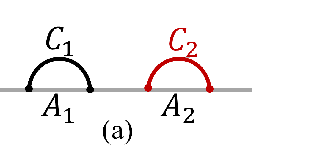
Though every brane will backreact on the bulk geometry, the interaction between two branes will be suppressed. Thus, up to the leading order of $x$, the final result would be simply twice of a single brane. The intrinsic refined trace distance in this case becomes

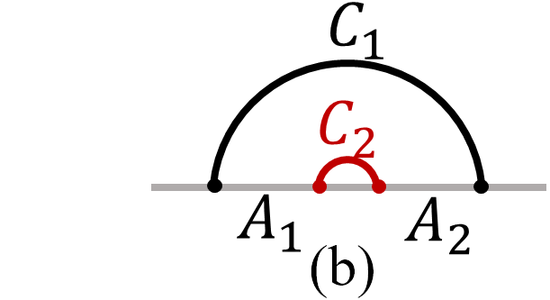
For large cross ration $x\rightarrow 1$, the configuration of two cosmic branes is shown in subfigure (b) of Fig. 1. The second cosmic brane $C_{2}$ will shrink into the boundary and two brane will also decouple with each other. As the result, we can compute two branes separately and obtain

Comparing with Eq. (28), we see that two limits have a symmetry $x\rightarrow 1-x$. Note that the computation here only involves the leading terms of $x\rightarrow 0$ or $x\rightarrow 1$. It will be interesting to study what will happen if the interaction between two branes cannot be neglected in the future.

To summary, this paper studies the holographic dualities of three most frequently-used quantum distances and a quantum quasi-distance, i.e. the trace distance, Fubini-Study distance, Bures distance and Rényi relative entropy. By choosing the modular vacuum as the reference state, it finds that they all have holographic dualities. Then it applies these holographic dualities into 2-dimensional CFTs and show that holographic results exactly match with the calculations of field theory.

For the holographic formula (9), there is no difficulty to obtain generalizations to theories dual to higher derivative gravity. The basic idea is similar to the directions of Refs. Dong:2013qoa ; Camps:2013zua ; Miao:2014nxa . The area term in right-hand side of Eq. (9) should be replaced by the Wald entropy Wald:1993nt evaluated on a cosmic brane. In addition, following the methods of Faulkner:2013ana ; Engelhardt:2014gca we can also include quantum corrections into Eq. (11) by taking the bulk matters into account. For 2 dimensional CFT with 2+1 dimensional gravity duality, it is also interesting to consider the perturbational expansion of small cross ration in gravity side by taking the interaction of two cosmic branes and then compare it with the results of CFTs.

References

- (1) J. M. Maldacena, The Large N limit of superconformal field theories and supergravity, Int. J. Theor. Phys. 38 (1999) 1113–1133, [hep-th/9711200].
- (2) S. Gubser, I. R. Klebanov and A. M. Polyakov, Gauge theory correlators from noncritical string theory, Phys. Lett. B 428 (1998) 105–114, [hep-th/9802109].
- (3) E. Witten, Anti-de Sitter space and holography, Adv. Theor. Math. Phys. 2 (1998) 253–291, [hep-th/9802150].
- (4) S. Ryu and T. Takayanagi, Holographic derivation of entanglement entropy from AdS/CFT, Phys. Rev. Lett. 96 (2006) 181602, [hep-th/0603001].
- (5) V. E. Hubeny, M. Rangamani and T. Takayanagi, A Covariant holographic entanglement entropy proposal, JHEP 07 (2007) 062, [0705.0016].
- (6) B. Chen, Holographic Entanglement Entropy: A Topical Review, Commun. Theor. Phys. 71 (2019) 837.
- (7) L.-Y. Hung, R. C. Myers, M. Smolkin and A. Yale, Holographic Calculations of Renyi Entropy, JHEP 12 (2011) 047, [1110.1084].
- (8) X. Dong, The Gravity Dual of Renyi Entropy, Nature Commun. 7 (2016) 12472, [1601.06788].
- (9) X. Dong, Holographic Entanglement Entropy for General Higher Derivative Gravity, JHEP 01 (2014) 044, [1310.5713].
- (10) J. Camps, Generalized entropy and higher derivative Gravity, JHEP 03 (2014) 070, [1310.6659].
- (11) R.-X. Miao and W.-Z. Guo, Holographic Entanglement Entropy for the Most General Higher Derivative Gravity, JHEP 08 (2015) 031, [1411.5579].
- (12) T. Faulkner, A. Lewkowycz and J. Maldacena, Quantum corrections to holographic entanglement entropy, JHEP 11 (2013) 074, [1307.2892].
- (13) N. Engelhardt and A. C. Wall, Quantum Extremal Surfaces: Holographic Entanglement Entropy beyond the Classical Regime, JHEP 01 (2015) 073, [1408.3203].
- (14) D. Harlow and P. Hayden, Quantum Computation vs. Firewalls, JHEP 06 (2013) 085, [1301.4504].
- (15) D. Stanford and L. Susskind, Complexity and Shock Wave Geometries, Phys. Rev. D 90 (2014) 126007, [1406.2678].
- (16) L. Susskind, Computational Complexity and Black Hole Horizons, Fortsch. Phys. 64 (2016) 24–43, [1403.5695].
- (17) A. R. Brown, D. A. Roberts, L. Susskind, B. Swingle and Y. Zhao, Holographic Complexity Equals Bulk Action?, Phys. Rev. Lett. 116 (2016) 191301, [1509.07876].
- (18) B. Czech, Einstein Equations from Varying Complexity, Phys. Rev. Lett. 120 (2018) 031601, [1706.00965].
- (19) P. Caputa and J. M. Magan, Quantum Computation as Gravity, Phys. Rev. Lett. 122 (2019) 231302, [1807.04422].
- (20) L. Susskind and Y. Zhao, Switchbacks and the Bridge to Nowhere, 1408.2823.
- (21) M. A. Nielsen and I. L. Chuang, Quantum Computation and Quantum Information: 10th Anniversary Edition. Cambridge University Press, Cambridge, UK, 10th ed., 2011.
- (22) J. Watrous, The Theory of Quantum Information. Cambridge University Press, Cambridge, UK, 1st ed., 2018.
- (23) N. Lashkari, Relative entropies in conformal field theory, Phys. Rev. Lett. 113 (Jul, 2014) 051602.
- (24) J. Zhang, P. Ruggiero and P. Calabrese, Subsystem Trace Distance in Quantum Field Theory, Phys. Rev. Lett. 122 (2019) 141602, [1901.10993].
- (25) J. Zhang, P. Ruggiero and P. Calabrese, Subsystem trace distance in low-lying states of -dimensional conformal field theories, JHEP 10 (2019) 181, [1907.04332].
- (26) J. Zhang and P. Calabrese, Subsystem distance after a local operator quench, JHEP 02 (2020) 056, [1911.04797].
- (27) D. D. Blanco, H. Casini, L.-Y. Hung and R. C. Myers, Relative Entropy and Holography, JHEP 08 (2013) 060, [1305.3182].
- (28) M. Miyaji, T. Numasawa, N. Shiba, T. Takayanagi and K. Watanabe, Distance between quantum states and gauge-gravity duality, Phys. Rev. Lett. 115 (Dec, 2015) 261602.
- (29) M. Alishahiha and A. Faraji Astaneh, Holographic fidelity susceptibility, Phys. Rev. D 96 (Oct, 2017) 086004.
- (30) E. J. König, A. Levchenko and N. Sedlmayr, Universal fidelity near quantum and topological phase transitions in finite one-dimensional systems, Phys. Rev. B 93 (Jun, 2016) 235160.
- (31) P. Zanardi, M. Cozzini and P. Giorda, Ground state fidelity and quantum phase transitions in free fermi systems, Journal of Statistical Mechanics: Theory and Experiment 2007 (Feb., 2007) L02002–L02002.
- (32) R. Haag, Local quantum physics: Fields, particles, algebras. Springer, Berlin, Germany, 05, 1992.
- (33) H. Li and F. D. M. Haldane, Entanglement spectrum as a generalization of entanglement entropy: Identification of topological order in non-abelian fractional quantum hall effect states, Phys. Rev. Lett. 101 (Jul, 2008) 010504.
- (34) H. Yao and X.-L. Qi, Entanglement entropy and entanglement spectrum of the kitaev model, Phys. Rev. Lett. 105 (Aug, 2010) 080501.
- (35) A. Lewkowycz and J. Maldacena, Generalized gravitational entropy, Journal of High Energy Physics 2013 (Aug., 2013) .
- (36) M. Müller-Lennert, F. Dupuis, O. Szehr, S. Fehr and M. Tomamichel, On quantum rényi entropies: A new generalization and some properties, Journal of Mathematical Physics 54 (2013) 122203, [https://doi.org/10.1063/1.4838856].
- (37) M. M. Wilde, A. Winter and D. Yang, Strong converse for the classical capacity of entanglement-breaking and hadamard channels via a sandwiched rényi relative entropy, Communications in Mathematical Physics 331 (July, 2014) 593–622.
- (38) Y. Nakaguchi and T. Nishioka, A holographic proof of Rényi entropic inequalities, JHEP 12 (2016) 129, [1606.08443].
- (39) R. M. Wald, Black hole entropy is the Noether charge, Phys. Rev. D 48 (1993) 3427–3431, [gr-qc/9307038].