Greedy Sensor Selection for Weighted Linear Least Squares Estimation under Correlated Noise
Abstract
Optimization of sensor selection has been studied to monitor complex and large-scale systems with data-driven linear reduced-order modeling. An algorithm for greedy sensor selection is presented under the assumption of correlated noise in the sensor signals. A noise model is given using truncated modes in reduced-order modeling, and sensor positions that are optimal for generalized least squares estimation are selected. The determinant of the covariance matrix of the estimation error is minimized by efficient one-rank computations in both underdetermined and overdetermined problems. The present study also reveals that the objective function with correlated noise is neither submodular nor supermodular. Several numerical experiments are conducted using randomly generated data and real-world data. The results show the effectiveness of the selection algorithm in terms of accuracy in the estimation of the states of large-dimensional measurement data.
1 Introduction
Observation is the primal step toward understanding real-world phenomena. When monitoring quantities that cannot be observed directly, system representations are constructed for describing the dynamical behavior of the phenomena of interest as the state space of physical equations including unknown parameters. Therefore, parameter estimation using sensor measurements has long attracted attention in many engineering and scientific applications [63, 2, 28, 60, 29, 65]. A reduction in the number of measurements is concurrently demanded for more practical use, especially under resource constraints on sensors and communication energy, or for processing measurements in real time. Optimization problems are presented here using metrics defined for sensor locations. The Fisher information matrix is a well-used metric for the assessment of uncertainty in parameter estimation, as this optimization task is closely related to the experimental designs [26, 4, 43]. The theory of information and statistics are also informative criteria for the optimization task [9, 30, 15, 44, 54].
Sensor placement based on the physical equations has been adopted in the reconstruction of physical fields, such as sound or seismic wave distribution [12, 13, 57]. With a similar formulation of the placement, sensor selection has been conducted by choosing the best subset of sensor nodes in the context of network monitoring and target tracking [46, 1]. Recently, advances in data-driven techniques enable us to obtain a system representation from astonishingly high dimensional monitoring data for complex phenomena, with sensor nodes defined by each sampling point in the data [5, 53, 48, 7, 31, 8, 19]. Spatiotemporal correlations between measurements at sensor nodes are here represented as a superposition of a limited number of bases, sometimes with impositions of a physical structure or robustness to the system [3, 58, 52, 6]. The use of optimized measurement has been accelerating the applications of data-driven modeling in several engineering fields such as face recognition [33], inbetweening of non-time-resoloved data [59], noise reduction [20], state estimation for air flow [24], wind orientation detection for vehicles [18], and source localization [25].
The main challenge of such optimization problems is intractability, where the problems are often classified as being nondeterministic polynomial-time hard. Therefore, heuristics to find suboptimal solutions have been intensely discussed. For example, the selection problem is solved by the linear convex relaxation methods [23, 42, 10] or by using proximal gradient methods [11, 35]. The submodularity property in these optimization problems also encourages the use of greedy algorithms [40, 14, 16, 17, 49, 50, 51]. Some recent studies attempt to improve the performance of greedy algorithms by grouping and multiobejective strategies, which considers multiple sensor subsets simultaneously [22, 36, 39].
Despite these established methodologies, considering the complex structure of measurement noise still remains a great challenge for the sensor selection problem, as treated in recent studies [45, 21, 34, 47]. The discrepancy between measurements and the model should be surely considered as spatially correlated measurement noise, for example, due to numerical computation of equations and assumptions in the modeling [27, 66], or due to truncation in the model order reduction [64, 37]. These errors cause correlated effects on the estimation adversely, thus the evaluation of the measurement noise should be included in the sensor selection objective. As previously illustrated by Ucinski [61], a sensor selection problem with continuous relaxation loses convexity when the noise covariance term is introduced. Liu et al. [32] put forward a semidefinite programming for the sensor selection problem with spatially correlated noise, but the calculation becomes prohibitive due to the large problem size. The greedy algorithm introduced in this study smoothly integrates the noise covariance into the formulation in Saito et al. [50], although the loss of submodularity is also confirmed. Another advantage of greedy methods is to circumvent the rounding procedures for obtaining sensor positions from a relaxed solution, which are still an arguable process especially under the nonconvexity of the optimized objective function.
The objective functions for the greedy selection are derived in both of the overdetermined and underdetermined settings, which generalize the previous D-optimality-based formulation [50]. The Fisher information matrix is defined in this work to evaluate the uncertainty of linear least squares estimation for a static system. The algorithm leverages one-rank computation for both a sensitivity term for each sensor and a weighting term for measurement noise. Some of the recent studies introduced prior distribution for Bayesian estimation [32, 64], maximum a posteriori estimation [55], and Kalman filtering [67]. Virtually, the hyper parameters in those distributions must be optimized using some information criteria or cross-validation techniques. The formulation in the present study excludes a prior distribution, because the optimization for hyperparameters is difficult for high dimensional data treated in subsection 3.2. In summary, we herein 1) propose an optimization problem for greedy sensor selection generalized for correlated measurement noise, which is easily extended to various optimality criteria, 2) confirm that the objective function is neither submodular nor supermodular, and 3) formulate a fast greedy algorithm that selects sensors optimized for both underdetermined and overdetermined cases in the weighted linear least squares estimation.
2 Formulation and Algorithm
This section describes problem settings for sensor selection tailored for weighted least squares estimation. Then, algorithms for greedy selection are discussed.
2.1 Sparse Sensing
A linear measurement equation for sensors and a state vector of components is corrupted by Gaussian noise , which is independent of ,
| (1) |
We assume that the sensor characteristic is known in advance and nonsingular, and the covariance of the measurement noise is positive definite and symmetric. An parameter vector is estimated from Eq. 1:
| (2a) | |||||
| , | (2b) |
Note that Eq. (2a) corresponds to the minimal norm solution in which the measurement noise is not considered, though Eq. (2a) is derived from the formulation including measurement noise. On the other hand, Eq. (2b) is a minimum variance unbiased estimation considering measurement noise as the generalized least squares estimation [56, Section 4.5]. The present study focuses on the formulation above, excluding any prior distribution of the state variables.
We also assume a large number of possible measurement points, e.g., . The linear coefficients and noise covariance for all of the measurement points are expressed as and , respectively. Actual calculations for these terms are introduced later herein at subsection 2.2. With these notations, the measurement is expressed by substituting . Here, the estimation Eq. 2a is redundant if is small, and thus the reduced measurement is sufficient in terms of both estimation quality and calculation efficiency. A sensor indication matrix is defined for a set of sensor indices selected from candidates. The position of unity in the -th row of is associated with the -th component of , whereas the rest of the row is zero. Measurements and linear coefficients for the selected sensors are denoted as and , respectively. In addition, the covariance matrix for measurement noise is expressed by . The argument will be denoted as subscript for brevity hereinafter.
2.2 Data-driven modeling
In our implementation, the matrices and are generated by modal decomposition of the collected data matrix, in a process known as principal component analysis, or proper orthogonal decomposition [7, 33]. The collected data are assumed to consist of -point measurements in rows by instances in columns, where . is decomposed by singular value decomposition into orthonormal spatial modes and temporal modes , and a diagonal matrix of singular values . The approximation mode number is chosen to retain the covariance matrix for the original data matrix at a high rate:
| (3) |
where and , and , and , respectively. Here, the second term with the subscript on the right-hand side is the portion that is excluded from rank representation and thus is regarded as the measurement noise. The -th column of and are the variable vector and the measurement in Eq. 1 for the -th instance, respectively. Thus, one can immediately recover the low rank representation of the large-scale measurement as by obtaining an estimation [33]. With respect to , several approaches are capable of expressing the statistical behavior of the residual between the measurement and the reduced order model, , which are exemplified by kernel functions used in signal processing or data-driven modeling in Ref. [64, Section 2]. By taking the expectation , the model of noise in the latter manner is denoted as of Eq. 3, which is used in section 3. Appendix A shows how the data-driven design of the measurement noise covariance is affected in the standpoint of the correlation and amount of training data.
2.3 Objective function for sensor selection
Several criteria for sensor selection are available for scalar evaluation of the measurement design, like D-, E- or A-optimality mentioned in [62].The performances for D-, E- and A-optimality criteria were previously compared for sensor sets obtained by greedy sensor selection methods suited for these criteria [38]. Sensor selection based on the D-optimality criterion performed well in both of the computational time and the values of other criteria, thus being adopted in the present study. Note that the efficient implementation shown in subsection 2.4 can easily be extended to the A-optimality settings.
Geometrically, this optimization corresponds to the minimization of the volume of an ellipsoid, which represents the expected estimation error variance [23]:
| (4) |
where the operator means taking the expected value of the argument. Furthermore, this matrix is known to correspond to the inverse of the Fisher information matrix. This equality is easily confirmed under the assumption of Gaussian measurement noise, by differentiating by a log likelihood, , then substituting estimation given by Eq.(2b). The optimization returns the set of measurement point from all the possible locations, although this is normally an intractable process. Instead, a greedy algorithm is employed with objective functions for both and . They are derived by generalizing the formulation in Ref. [38] for the correlated measurement noise hereafter. The set of sensors are evaluated only in the observable subspace of , since the measurement system Eq. 1 is underdetermined when . From Eq. 4, the subspace is separated by the projection after singular value decomposition of :
| (7) |
with some matrices of appropriate dimensions,
| (16) |
The evaluation of the error covariance in the observable subspace was recently introduced by Nakai et al. [38], and it is extended to the correlated noise case in the present study for the first time (to the best of our knowledge). One can use various metrics for the projected covariance matrix Eq. 7 like its determinant, trace or minimum eigenvalue, as in Ref. [23, 38]. The determinant of the inverse matrices in Eq. 7 is maximized in the present manuscript:
| (17a) | |||||
| . | (17b) |
Note that whitening all candidates with before sensor selection is based on the assumption of weakly correlated noise, because contains noise covariance over sensors that are not selected as pointed out in [32]. In subsection 2.4, an algorithm is presented for achieving Eq. 17b in a greedy manner.
2.4 Efficient greedy algorithm
Algorithm 1 shows the procedure implemented in the computation conducted in section 3, which implicitly exploits the one-rank determinant lemma as [32, 50, 64]. It is worth mentioning that the previously presented noise-ignoring algorithm in [50], Algorithm 2, is easily obtained by substituting an identity matrix into .
The equations are converted by the lemma shown later herein. First, consider an objective function when there are fewer sensors deployed than the number of state variables :
| (18) |
where the subscript represents the component produced by the -th sensor candidate in the -th step:
Here, is the -th row of , and and are the noise covariance between the selected sensors given by the previous steps and the -th candidate and noise variance for the -th candidate, respectively. The algorithm avoids expensive computations involving the determinant by separating the components of the obtained sensors from the objective function in the current selection step of Eq. 18:
| (19) |
and then a unit vector , of which only the -th entry is unity, is added to the -th row of . Note that Eq. 19 corresponds to maximization of the difference when an arbitrary sensor is added to the sensor set of the previous step. The numerator of Eq. 19 is the norm of the vector, and the denominator is positive, because the covariance matrix is assumed to be positive definite. Subsequently, the objective function is modified for the case in which more sensors than the number of state variables have already been determined:
| (20) |
where Eq. 20 is positive, and the objective function, Eq. (17b), increases monotonically. Details of the expansion are found in Ref. [64].
The computational cost of algorithms are listed in Table 1:
The objective function loses submodularity if the measurement noises at different sensor positions are strongly correlated with each other (or when the off-diagonal components in are no smaller than the diagonal components.) The following example provides a nonsubmodular and nonsupermodular case for Eq. (17b). For simplicity, the spatial modes and the noise covariance are set as follows. Here, the noise components are strongly correlated, whereas those for are relatively independent.
| (27) |
With these matrices, the values of the determinant function Eq. (17b) are
where refers to the value of the determinant Eq. (17b) for the power sets of selected sensors. This example immediately shows that the objective function Eq. (17b) has neither submodularity nor supermodularity, whereas submodularity exists for the case with equally distributed uncorrelated measurement noise [50]. Thus, the sensor selection problem Eq. (17b) with a greedy method generally has no performance guarantee based on submodularity or supermodularity.
3 Results
This section describes some experiments that validate the algorithm. First, data matrices are constructed from randomly generated orthonormal bases. The NOAA-SST dataset [41] shows the results of a practical application.
3.1 Randomly generated data matrix
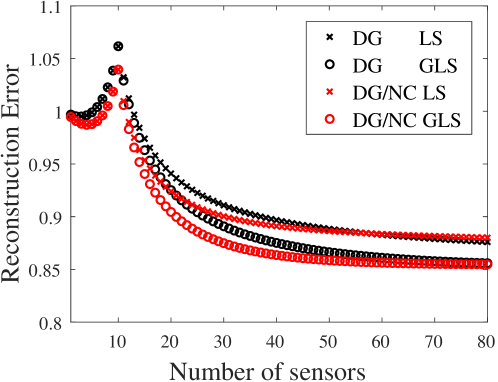
Generalized results are shown in this subsection. The problem considered here is as follows: a data matrix is constructed as , where and are and orthonormal matrices, respectively, generated from appropriately sized matrices containing numbers from a standard normal distribution, and is a diagonal matrix with . The algorithms for the sensor selection treat these matrices after dividing the first 10 columns as and and the remaining columns as and . Then, the first 10 diagonal components and the remaining are labeled as and , respectively. Note that the measure in terms of “reconstruction error” is expressed as Here, the series for the estimation of Eq. 2a is concatenated as , and represents the Frobenius norm of . Figure 1 shows the result of the reconstruction with the estimate with sensors and the dimensional reduced-order model Eq. 3. Here, DG and DG/NC in the legend refer to “determinant-based greedy algorithm” in Ref. [50] and Algorithm 1 considering “noise covariance” in the measurement, respectively, and LS and GLS refer to “linear least squares estimation” and “generalized linear least squares estimation” using noise covariance, respectively. Note that the plots for are calculated by the same estimator Eq. (2a), and, therefore, the estimations with a small number of sensors for both GLS and LS are identical for each selected sensor set. First, the GLS estimation reduces the reconstruction error in oversampling cases for sensors for both algorithms. The measurement noise is quite excessive, and thus, sensors of both selection methods exhibit comparable results for the LS estimation. Second, the more sensors are deployed, the lower the reduction becomes thanks to the GLS estimation. This is partly because measurement using a large number of sensors suppresses outliers resulting from the correlated measurement noise. If a much larger number of sensors is available than the number of estimated variables, the importance of correlation in the measurement noise might diminish.
3.2 NOAA-SST
Here, we apply this strategy to pursue sensor selection using large-dimensional climate data. A brief description of the NOAA-SST data is given in Table 2.
| Label | NOAA Optimum Interpolation (OI) SST V2 [41] |
| Temporal Coverage | Weekly means from 1989/12/31 to 1999/12/12 ( snapshots) |
| Spatial Coverage | 1.0 degree latitude 1.0 degree longitude global grid ( measurement on the ocean) |
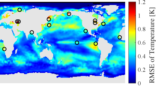
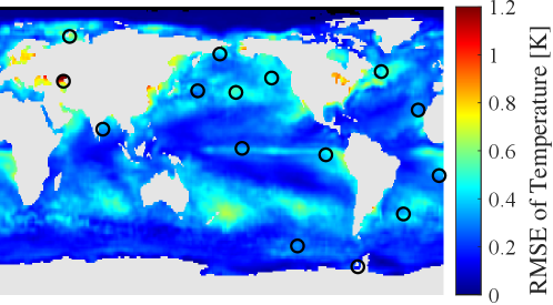
Similar to subsection 3.1, orthonormal modes are prepared by conducting SVD on the data matrix with the average being subtracted, then the first 10 of the 520 modes are used to build the reduced-order model of the temperature distribution (). The remaining modes are used for the noise covariance matrix. Several sensor positions for which the noise amplitude is extremely low (smaller than 1% of the maximum RMS of noise in this comparison) are eliminated from candidate set beforehand, as conducted in [64]. The results in this subsection can be compared with those in Ref. [33], [64], or [50]. In Fig. 2, the positions of sensors are represented by open circles on the colored maps, which illustrate the fluctuation of estimation error using those sensors, namely . The difference in the sensor positions is remarkable, since the proposed algorithm spreads sensors and avoids neighboring sensors that might be affected by correlated measurement noise. The reduction in the estimation error is also recognizable by comparing the backgrounds.
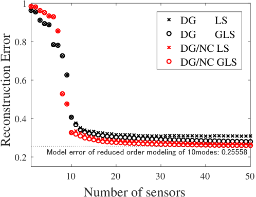
Figure 3 compares the results of estimation using the noise covariance information. Note that cross-validation is not conducted for this comparison, since it is hard to quantify the estimation error because of the dynamics in SST which is partly extracted by the reduced order modeling. In appendix A, the covariance matrix of measurement noise is characterized by the number of snapshots to form the noise covariance matrix. A horizontal broken line in Fig. 3 shows the modeling error due to the low-rank representation of Eq. 3. The red plots show better performance for sensors using the proposed algorithm than those using the previous DG algorithm [50] owing to the noise covariance matrix in the sensor selection procedure. There are several differences in the trend of plots compared to Fig. 1, e.g. the contribution from sensors of the proposed algorithm is more significant than that for the GLS estimation. This is perhaps because of the weak amplitude of higher ordered modes in addition to the similarity in the location where the reduced-order phenomena and the measurement noise fluctuates greatly. The proposed algorithm that involves noise covariance evaluates the positions with less measurement noise. Therefore, accurate estimation is achieved even with linear least squares estimation, which contrasts with the errors of sensors of DG algorithm staying relatively high.
4 Conclusions
A greedy algorithm for sensor selection for generalized least squares estimation is presented. A covariance matrix generated by truncated modes in reduced-order modeling is applied and a weighting matrix is built for the estimation. A specialized one-rank lemma involving the covariance matrix realizes a simple transformation from the true optimization into a series of a greedy scalar evaluation. In addition, the objective function is shown to be neither submodular nor supermodular. Numerical tests using two kinds of datasets are performed to assess the proposed determinant-based optimization method. The proposed algorithm gives less noisy sensors and results in stable estimation in the presence of measurement noise from truncated modes of the reduced-order modeling.
Acknowledgements
The present study was supported by JSPS KAKENHI (21J20671), JST ACT-X (JPMJAX20AD), JST CREST (JPMJCR1763) and JST FOREST (JPMJFR202C).
Appendix A Data-driven noise correlation in real-world data
In this section, some numerical experiments are conducted and the data dependency of the data-driven modeling of the measurement noise are explored. Mainly impact of the number of the used snapshots is investigated in this section. Here, six-fold cross-validation is applied to 624 snapshots of the same NOAA-SST data used in subsection 3.2.
The procedure is summarized as follows:
-
1.
Save 624 snapshots in the memory of computer
-
2.
Calculate reduced order representation by Eq. 3
-
3.
Randomize the order of the snapshots and divide into six parts
-
4.
Sample the predetermined number of snapshots randomly from 520 snapshots labeled as “training” then calculate
-
5.
Determine 15 sensor positions using and
-
6.
Reconstruct all-points measurement of 104 snapshots labeled as “test” using determined sensors and corresponding
-
7.
Store reconstruction error
- 8.
- 9.
Here, the low-rank representation is fixed for all of the sampling cases, and the change in the reduced order representation which reflects temperature dynamics is excluded. An evaluation of the quality including the reduced order model needs more profound discussion, and thus, this topic remains to be solved. Calculation of noise correlation matrix in item 4 above is carried out by taking , where with some notations in subsections 2.1 and 2.2.
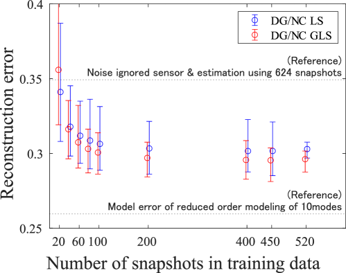
In Fig. 4, the result is summarized by the average, maximum, and minimum of the reconstruction error with the abscissa of the number of snapshots used as training data. Among the two horizontal broken lines, the top one corresponds to the average of the reconstruction error of six divided snapshots by the previous approach that only uses , and the bottom to the modeling error by approximating original snapshots by modes. The lack of the training data for calculating influences the reconstruction at 20 snapshots, possibly since the weighting term using measurement noise is not captured well. The presented method, however, results in better performance than the previous approach as the number of snapshots in the training data increases. For the further reduction in the reconstruction error, it seems effective to increase the number of sensors (as shown in section 3), or consider the dynamics of the measured phenomena to the estimation if the time-series snapshots are applied.
References
- [1] Charu C. Aggarwal, Amotz Bar-Noy, and Simon Shamoun. On sensor selection in linked information networks. Computer Networks, 126:100–113, 2017.
- [2] Antonio A Alonso, Christos E Frouzakis, and Ioannis G Kevrekidis. Optimal sensor placement for state reconstruction of distributed process systems. AIChE Journal, 50(7):1438–1452, 2004.
- [3] Peter J Baddoo, Benjamin Herrmann, Beverley J McKeon, J Nathan Kutz, and Steven L Brunton. Physics-informed dynamic mode decomposition (pidmd). arXiv preprint arXiv:2112.04307, 2021.
- [4] RA Bates, RJ Buck, E Riccomagno, and HP Wynn. Experimental design and observation for large systems. Journal of the Royal Statistical Society: Series B (Methodological), 58(1):77–94, 1996.
- [5] Gal Berkooz, Philip Holmes, and John L Lumley. The proper orthogonal decomposition in the analysis of turbulent flows. Annual review of fluid mechanics, 25(1):539–575, 1993.
- [6] Matthew Brand. Incremental singular value decomposition of uncertain data with missing values. In European Conference on Computer Vision, pages 707–720. Springer, 2002.
- [7] Steven L Brunton and J Nathan Kutz. Data-driven science and engineering: Machine learning, dynamical systems, and control. Cambridge University Press, 2019.
- [8] Steven L Brunton, Joshua L Proctor, Jonathan H Tu, and J Nathan Kutz. Compressed sensing and dynamic mode decomposition. Journal of Computational Dynamics, 2(2):165, 2015.
- [9] Sundeep Prabhakar Chepuri and Geert Leus. Sparse sensing for distributed detection. IEEE Transactions on Signal Processing, 64(6):1446–1460, 2015.
- [10] Donald J Chmielewski, Tasha Palmer, and Vasilios Manousiouthakis. On the theory of optimal sensor placement. AIChE journal, 48(5):1001–1012, 2002.
- [11] Neil K Dhingra, Mihailo R Jovanović, and Zhi-Quan Luo. An admm algorithm for optimal sensor and actuator selection. In 53rd IEEE Conference on Decision and Control, pages 4039–4044. IEEE, 2014.
- [12] Kutluyıl Doğançay and Hatem Hmam. On optimal sensor placement for time-difference-of-arrival localization utilizing uncertainty minimization. In 2009 17th European Signal Processing Conference, pages 1136–1140. IEEE, 2009.
- [13] Wan Du, Zikun Xing, Mo Li, Bingsheng He, Lloyd Hock Chye Chua, and Haiyan Miao. Optimal sensor placement and measurement of wind for water quality studies in urban reservoirs. In IPSN-14 Proceedings of the 13th International Symposium on Information Processing in Sensor Networks. IEEE, apr 2014.
- [14] Uriel Feige, Vahab S Mirrokni, and Jan Vondrák. Maximizing non-monotone submodular functions. SIAM Journal on Computing, 40(4):1133–1153, 2011.
- [15] Roman Garnett, Michael A Osborne, and Stephen J Roberts. Bayesian optimization for sensor set selection. In Proceedings of the 9th ACM/IEEE international conference on information processing in sensor networks, pages 209–219, 2010.
- [16] Daniel Golovin and Andreas Krause. Adaptive submodularity: Theory and applications in active learning and stochastic optimization. Journal of Artificial Intelligence Research, 42:427–486, 2011.
- [17] Abolfazl Hashemi, Mahsa Ghasemi, Haris Vikalo, and Ufuk Topcu. Randomized greedy sensor selection: Leveraging weak submodularity. IEEE Transactions on Automatic Control, 66(1):199–212, 2020.
- [18] Ryoma Inoba, Kazuki Uchida, Yuto Iwasaki, Takayuki Nagata, Yuta Ozawa, Yuji Saito, Taku Nonomura, and Keisuke Asai. Optimization of sparse sensor placement for estimation of wind direction and surface pressure distribution using time-averaged pressure-sensitive paint data on automobile model. Journal of Wind Engineering and Industrial Aerodynamics, submitted.
- [19] Tomoki Inoue, Tsubasa Ikami, Yasuhiro Egami, Hiroki Nagai, Yasuo Naganuma, Koichi Kimura, and Yu Matsuda. Data-driven optimal sensor placement for high-dimensional system using annealing machine. arXiv preprint arXiv:2205.05430e, 2022.
- [20] Tomoki Inoue, Yu Matsuda, Tsubasa Ikami, Taku Nonomura, Yasuhiro Egami, and Hiroki Nagai. Data-driven approach for noise reduction in pressure-sensitive paint data based on modal expansion and time-series data at optimally placed points. Physics of Fluids, 33(7):077105, 2021.
- [21] Hadi Jamali-Rad, Andrea Simonetto, Geert Leus, and Xiaoli Ma. Sparsity-aware sensor selection for correlated noise. In 17th International Conference on Information Fusion (FUSION), pages 1–7. IEEE, 2014.
- [22] C. Jiang, Z. Chen, R. Su, and Y. C. Soh. Group greedy method for sensor placement. IEEE Transactions on Signal Processing, 67(9):2249–2262, 2019.
- [23] Siddharth Joshi and Stephen Boyd. Sensor selection via convex optimization. IEEE Transactions on Signal Processing, 57(2):451–462, 2009.
- [24] Naoki Kanda, Kumi Nakai, Yuji Saito, Taku Nonomura, and Keisuke Asai. Feasibility study on real-time observation of flow velocity field using sparse processing particle image velocimetry. Transactions of the Japan Society for Aeronautical and Space Sciences, 64(4):242–245, 2021.
- [25] Sayumi Kaneko, Yuta Ozawa, Kumi Nakai, Yuji Saito, Taku Nonomura, Keisuke Asai, and Hiroki Ura. Data-driven sparse sampling for reconstruction of acoustic-wave characteristics used in aeroacoustic beamforming. Applied Sciences, 11(9):4216, 2021.
- [26] Rex K Kincaid and Sharon L Padula. D-optimal designs for sensor and actuator locations. Computers & Operations Research, 29(6):701–713, 2002.
- [27] R Kirlin and L Dewey. Optimal delay estimation in a multiple sensor array having spatially correlated noise. IEEE transactions on acoustics, speech, and signal processing, 33(6):1387–1396, 1985.
- [28] Toni Kraft, Arnaud Mignan, and Domenico Giardini. Optimization of a large-scale microseismic monitoring network in northern switzerland. Geophysical Journal International, 195(1):474–490, 2013.
- [29] Andreas Krause, Jure Leskovec, Carlos Guestrin, Jeanne VanBriesen, and Christos Faloutsos. Efficient sensor placement optimization for securing large water distribution networks. Journal of Water Resources Planning and Management, 134(6):516–526, 2008.
- [30] Andreas Krause, Ajit Singh, and Carlos Guestrin. Near-optimal sensor placements in gaussian processes: Theory, efficient algorithms and empirical studies. Journal of Machine Learning Research, 9(Feb):235–284, 2008.
- [31] J Nathan Kutz, Steven L Brunton, Bingni W Brunton, and Joshua L Proctor. Dynamic mode decomposition: data-driven modeling of complex systems. SIAM, 2016.
- [32] Sijia Liu, Sundeep Prabhakar Chepuri, Makan Fardad, Engin Maşazade, Geert Leus, and Pramod K Varshney. Sensor selection for estimation with correlated measurement noise. IEEE Transactions on Signal Processing, 64(13):3509–3522, 2016.
- [33] Krithika Manohar, Bingni W Brunton, J Nathan Kutz, and Steven L Brunton. Data-driven sparse sensor placement for reconstruction: Demonstrating the benefits of exploiting known patterns. IEEE Control Systems Magazine, 38(3):63–86, 2018.
- [34] Engin Masazade, Makan Fardad, and Pramod K Varshney. Sparsity-promoting extended kalman filtering for target tracking in wireless sensor networks. IEEE Signal Processing Letters, 19(12):845–848, 2012.
- [35] Takayuki Nagata, Taku Nonomura, Kumi Nakai, Keigo Yamada, Yuji Saito, and Shunsuke Ono. Data-driven sparse sensor selection based on a-optimal design of experiment with admm. IEEE Sensors Journal, 2021.
- [36] Takayuki Nagata, Keigo Yamada, Kumi Nakai, Yuji Saito, and Taku Nonomura. Randomized group-greedy method for data-driven sensor selection. IEEE Sensors Journal, submitted.
- [37] Takayuki Nagata, Keigo Yamada, Taku Nonomura, Kumi Nakai, Yuji Saito, and Shunsuke Ono. Data-driven sensor selection method based on proximal optimization for high-dimensional data with correlated measurement noise. arXiv preprint arXiv:2205.06067e, 2022.
- [38] K. Nakai, K. Yamada, T. Nagata, Y. Saito, and T. Nonomura. Effect of objective function on data-driven greedy sparse sensor optimization. IEEE Access, 9:46731–46743, 2021.
- [39] Kumi Nakai, Takayuki Nagata, Keigo Yamada, Yuji Saito, and Taku Nonomura. Nondominated-solution-based multiobjective-greedy sensor selection for optimal design of experiments. arXiv preprint arXiv:2204.12695e, 2022.
- [40] George L Nemhauser, Laurence A Wolsey, and Marshall L Fisher. An analysis of approximations for maximizing submodular set functions. Mathematical programming, 14(1):265–294, 1978.
- [41] NOAA/OAR/ESRL. Noaa optimal interpolation (oi) sea surface temperature (sst) v2.
- [42] T. Nonomura, S. Ono, K. Nakai, and Y. Saito. Randomized subspace newton convex method applied to data-driven sensor selection problem. IEEE Signal Processing Letters, 28:284–288, 2021.
- [43] S Padula, D Palumbo, and R Kincaid. Optimal sensor/actuator locations for active structural acoustic control. In 39th AIAA/ASME/ASCE/AHS/ASC Structures, Structural Dynamics, and Materials Conference and Exhibit, page 1865, 1998.
- [44] Romain Paris, Samir Beneddine, and Julien Dandois. Robust flow control and optimal sensor placement using deep reinforcement learning. Journal of Fluid Mechanics, 913, 2021.
- [45] Andrej Pázman and Werner G Müller. Optimal design of experiments subject to correlated errors. Statistics & probability letters, 52(1):29–34, 2001.
- [46] M.S. Phatak. Recursive method for optimum gps satellite selection. IEEE Transactions on Aerospace and Electronic Systems, 37(2):751–754, apr 2001.
- [47] Erik Rigtorp. Sensor selection with correlated noise. Master’s thesis, KTH Royal Institute of Tehcnology, 2010.
- [48] Clarence W Rowley, Tim Colonius, and Richard M Murray. Model reduction for compressible flows using pod and galerkin projection. Physica D: Nonlinear Phenomena, 189(1-2):115–129, 2004.
- [49] Yuji Saito, Taku Nonomura, Koki Nankai, Keigo Yamada, Keisuke Asai, Yasuo Sasaki, and Daisuke Tsubakino. Data-driven vector-measurement-sensor selection based on greedy algorithm. IEEE Sensors Letters, 4, 2020.
- [50] Yuji Saito, Taku Nonomura, Keigo Yamada, Kumi Nakai, Takayuki Nagata, Keisuke Asai, Yasuo Sasaki, and Daisuke Tsubakino. Determinant-based fast greedy sensor selection algorithm. IEEE Access, 9:68535–68551, 2021.
- [51] Yuji Saito, Keigo Yamada, Naoki Kanda, Kumi Nakai, Takayuki Nagata, Taku Nonomura, and Keisuke Asai. Data-driven determinant-based greedy under/oversampling vector sensor placement. CMES-COMPUTER MODELING IN ENGINEERING & SCIENCES, 129(1):1–30, 2021.
- [52] Isabel Scherl, Benjamin Strom, Jessica K Shang, Owen Williams, Brian L Polagye, and Steven L Brunton. Robust principal component analysis for modal decomposition of corrupt fluid flows. Physical Review Fluids, 5(5):054401, 2020.
- [53] P. J. Schmid. Dynamic mode decomposition of numerical and experimental data. Journal of Fluid Mechanics, 656(July 2010):5–28, 2010.
- [54] Richard Semaan. Optimal sensor placement using machine learning. Computers & Fluids, 159:167–176, 2017.
- [55] Manohar Shamaiah, Siddhartha Banerjee, and Haris Vikalo. Greedy sensor selection: Leveraging submodularity. In 49th IEEE conference on decision and control (CDC), pages 2572–2577. IEEE, 2010.
- [56] M Kay Steven. Fundamentals of statistical signal processing: Estimation Theory, volume 10. PTR Prentice-Hall, Englewood Cliffs, NJ, USA, 1993.
- [57] Mohammad J. Taghizadeh, Saeid Haghighatshoar, Afsaneh Asaei, Philip N. Garner, and Herve Bourlard. Robust microphone placement for source localization from noisy distance measurements. In 2015 IEEE International Conference on Acoustics, Speech and Signal Processing (ICASSP). IEEE, apr 2015.
- [58] Naoya Takeishi, Yoshinobu Kawahara, Yasuo Tabei, and Takehisa Yairi. Bayesian dynamic mode decomposition. In IJCAI, pages 2814–2821, 2017.
- [59] Jonathan H Tu, John Griffin, Adam Hart, Clarence W Rowley, Louis N Cattafesta, and Lawrence S Ukeiley. Integration of non-time-resolved piv and time-resolved velocity point sensors for dynamic estimation of velocity fields. Experiments in fluids, 54(2):1–20, 2013.
- [60] Vasileios Tzoumas, Yuankun Xue, Sérgio Pequito, Paul Bogdan, and George J Pappas. Selecting sensors in biological fractional-order systems. IEEE Transactions on Control of Network Systems, 5(2):709–721, 2018.
- [61] Dariusz Uciński. D-optimal sensor selection in the presence of correlated measurement noise. Measurement, 164:107873, 2020.
- [62] Firdaus E Udwadia. Methodology for optimum sensor locations for parameter identification in dynamic systems. Journal of engineering mechanics, 120(2):368–390, 1994.
- [63] Alain Vande Wouwer, Nicolas Point, Stephanie Porteman, and Marcel Remy. An approach to the selection of optimal sensor locations in distributed parameter systems. Journal of process control, 10(4):291–300, 2000.
- [64] Keigo Yamada, Yuji Saito, Koki Nankai, Taku Nonomura, Keisuke Asai, and Daisuke Tsubakino. Fast greedy optimization of sensor selection in measurement with correlated noise. Mechanical Systems and Signal Processing, 158:107619, 2021.
- [65] Ryoichi Yoshimura, Aiko Yakeno, Takashi Misaka, and Shigeru Obayashi. Application of observability gramian to targeted observation in wrf data assimilation. Tellus A: Dynamic Meteorology and Oceanography, 72(1):1–11, 2020.
- [66] Jing Yu, Victor M Zavala, and Mihai Anitescu. A scalable design of experiments framework for optimal sensor placement. Journal of Process Control, 67:44–55, 2018.
- [67] Armin Zare and Mihailo R Jovanović. Optimal sensor selection via proximal optimization algorithms. In 2018 IEEE Conference on Decision and Control (CDC), pages 6514–6518. IEEE, 2018.