ifaamas \acmDOIdoi \acmISBN \acmConference[AAMAS’20]Proc. of the 19th International Conference on Autonomous Agents and Multiagent Systems (AAMAS 2020), B. An, N. Yorke-Smith, A. El Fallah Seghrouchni, G. Sukthankar (eds.)May 2020Auckland, New Zealand \acmYear2020 \copyrightyear2020 \acmPrice
University of Southern California
Carnegie Mellon University
Carnegie Mellon University
Carnegie Mellon University \affiliation \institutionWorld Wildlife Fund \affiliation \institutionCarnegie Mellon University
Green Security Game with Community Engagement
Abstract.
While game-theoretic models and algorithms have been developed to combat illegal activities, such as poaching and over-fishing, in green security domains, none of the existing work considers the crucial aspect of community engagement: community members are recruited by law enforcement as informants and can provide valuable tips, e.g., the location of ongoing illegal activities, to assist patrols. We fill this gap and (i) introduce a novel two-stage security game model for community engagement, with a bipartite graph representing the informant-attacker social network and a level- response model for attackers inspired by cognitive hierarchy; (ii) provide complexity results and exact, approximate, and heuristic algorithms for selecting informants and allocating patrollers against level- () attackers; (iii) provide a novel algorithm to find the optimal defender strategy against level- attackers, which converts the problem of optimizing a parameterized fixed-point to a bi-level optimization problem, where the inner level is just a linear program, and the outer level has only a linear number of variables and a single linear constraint. We also evaluate the algorithms through extensive experiments.
Key words and phrases:
Security Game; Computational Sustainability; Community Engagement1. Introduction
Despite the significance of protecting natural resources to environmental sustainability, a common lack of funding leads to an extremely low density of law enforcement units (referred to as defenders) to combat illegal activities such as wildlife poaching and overfishing (referred to as attacks). Due to insufficient sanctions, attackers are able to launch frequent attacks Le Gallic and Cox (2006); Leader-Williams and Milner-Gulland (1993), making it even more challenging to effectively detect and deter criminal activities through patrolling. To improve patrol efficiency, law enforcement agencies often recruit informants from local communities and plan defensive resources based on tips provided by them Linkie et al. (2015). Since attackers are often from the same local community and their activities can be observed by informants through social interactions, such tips contain detailed information about ongoing or upcoming criminal activities and, if known by defenders, can directly be used to guide allocating defensive resources. In fact, community engagement is listed by World Wild Fund for Nature as one of the six pillars towards zero poaching WWF (2015). The importance of community engagement goes beyond these green security domains about environment conservation and extends to domains such as fighting urban crimes Tublitz and Lawrence (2014); Gill et al. (2014).
Previous research in computational game theory have led to models and algorithms that can help the defenders allocate limited resources in the presence of attackers, with applications to enforce traffic Rosenfeld and Kraus (2017), combat oil-siphoning Wang et al. (2018), and deceive cyber adversaries Schlenker et al. (2018) in addition to protecting critical infrastructure Pita et al. (2008) and combating wildlife crime Fang et al. (2017). However, none of the work has considered this essential element of community engagement.
Community engagement leads to fundamentally new challenges that do not exist in previous literature. First, the defender not only needs to determine how to patrol but also needs to decide whom to recruit as informants. Second, there can be multiple attackers, and the existence of informants makes the success or failure of their attacks interdependent since any tip about other attackers’ actions can change the defender’s patrol. Third, because of the combinatorial nature of the tips, representing the defender’s strategy requires exponential space, making the problem of finding optimal defender strategy extremely challenging. Fourth, attackers may notice the patrol pattern over time and adapt their strategies accordingly.
In this paper, we provide the first study to fill the gap and provide a novel two-stage security game model for community engagement which represents the social network between potential informants and attackers with a bipartite graph. In the first stage of the game, the defender recruits a set of informants under a budget constraint, and in the second stage, the defender chooses a set of targets to protect based on tips from recruited informants. Inspired by the quantal cognitive hierarchy model Wright and Leyton-Brown (2014), we use a level- response model for attackers, taking into account the fact that the attacker can make iterative reasoning and the attacker’s strategy will impact the actual marginal strategy of the defender.
Our second contribution includes complexity results and algorithms for computing optimal defender strategy against level- () attackers. We show that the problem of selecting the optimal set of informants is NP-Hard. Further, based on sampling techniques, we develop an approximation algorithm to compute the optimal patrol strategy and a heuristic algorithm to find the optimal set of informants to recruit. For an expository purpose, we mainly describe the algorithms for level-0 attackers and provide the extension to level- () attackers in the last section.
The third contribution is a novel algorithm to find the optimal defender strategy against level- attackers, which is an extremely challenging task: an attacker’s strategy may affect the defender’s marginal strategy, which in turn affects the attackers’ strategies and level- attackers is defined through a fixed-point argument; as a result, the defender’s utility relies crucially on solving a parameterized fixed-point problem. A naïve mathematical programming-based formulation is prohibitively large to solve. We instead reduce the program to a bi-level optimization problem, where both levels become more tractable. In particular, the inner level optimization is a linear program, and the outer level optimization is one with a linear number of variables and a single linear constraint.
Finally, we conduct extensive experiments. We compare the running time and solution quality of different algorithms. We show that our bi-level optimization algorithm achieves better performance than the algorithm adapted from previous works. We also compare level-0 attackers and the case with insider threat (i.e., the attacker is aware of the informants), where we formulate the problem as a mathematical program and solve it by adapting an algorithm from previous works. We show that the defender suffers from utility loss if the insider threat is not taken into consideration and the defender still assumes a naïve attacker model (level-0).
2. Related Work and Background
Community engagement is studied in criminology. Smith and Humphreys (2015); Moreto (2015); Duffy et al. (2015) investigate the role of community engagement in wildlife conservation. Linkie et al. (2015); Gill et al. (2014) show the positive effects of community-oriented strategies. However, they lack a mathematical model for strategic defender-attacker interactions.
Recruitment of informants has also been proposed to study societal attitudes in relation to crimes using evolutionary game theory models. Short et al. (2013) formulate the problem of solving recruitment strategies as an optimal control problem to account for limited resources and budget. In contrast to their work, we emphasize the synergy of community engagement and allocation of defensive resources and aim to find the best strategy of recruiting informants and allocating defensive resources.
In security domains, Stackelberg Security Game (SSG) has been applied to a variety of security problems Tambe (2011), with variants accounting for alarm systems, surveillance cameras, and drones that can provide information in real time Basilico et al. (2017); Ma et al. (2018); Guo et al. (2017). Unlike the sensors that provide location-based information as studied in previous works, the kind of tips the informants can provide depends on their social connections, an essential feature about community engagement.
Other than the full rationality model, boundedly rational behavioral models such as quantal response (QR) McKelvey and Palfrey (1995); Yang et al. (2012) and subjective utility quantal response Nguyen et al. (2013) have been explored in the study of SSG. Our model and solution approach are compatible with most existing behavioral models in the SSG literature, but for an expository purpose, we only focus on the QR model.
3. Model
In this section, we introduce our novel two-stage green security game with community engagement. The key addition is the consideration of informants from local communities. They can be recruited and trained by the defender to provide tips about ongoing or upcoming attacks.
Following existing works on SSG Jain et al. (2010); Korzhyk et al. (2011), we consider a game with a set of targets . The defender has units of defensive resources and each can protect or cover one target with no scheduling constraint. An attacker can choose a target to attack. If target is attacked, the defender (attacker) receives () if it is covered, otherwise receives ().
Informants recruited by the defender can provide tips regarding the exact targets in ongoing or upcoming attacks but tip frequency and usefulness may vary due to heterogeneity in the informants’ social connections. We model the interactions and connections between potential informants (i.e., members of the community that are known to be non-attacker and can be recruited by the defender) and potential attackers using a bipartite graph with . Here we assume the defender has access to a list of potential attackers which could be provided by the conservation site manager, since the deployment of our work relies on the manager’s domain knowledge, experience, and understanding of the social connections among community members.
When an attacker decides to launch an attack, an informant who interacted with the attacker previously may know his target location. Formally, for each , we assume that will attack a target with probability but the target is unknown without informants and each attacker takes actions independently. An edge is associated with an information sharing intensity , representing the probability of attack activities of attacker being reported by , given attacks and is recruited as an informant.
In the first stage, the defender recruits informants, and in the second stage, the defender receives tips from the informants and allocates units of defensive resources. The defender’s goal is to maximize the expected utility defined as the summation of the utilities for each attack.
Let denote the set of recruited informants in the first stage where , and denote the set of attackers that are connected with at least one informant in . We represent tips as a vector of disjoint subsets of attackers , where is the set of attackers who are reported to attack target such that for any . An attacker is reported if there exists such that , otherwise he is unreported. We also denote by the set of reported attackers. It is possible that and we say the defender is informed if . Note that is a compact representation of the tips received by the defender as it neglects the identity of the informants, which is not crucial in the defender’s decision making given that all the tips are assumed to be correct.
In practice, tips are infrequent and the defender is often very protective of the informants. Thus, the attackers are often not aware of the existence of informants unless there is a significant insider threat. In addition, patrols can be divided into two categories – routine patrols and ambush patrols, where the latter are in response to tips from informants. Ambush patrols are costly, often requiring rangers to lie in wait for many hours for the possibility of catching a poacher. If not informed, the defender follows her routine patrol strategy with denoting the probability that target is covered. Naturally, under this assumption the defender should use a strategy that is optimal against the QR model, which can be computed by following Yang et al. (2012). If informed she uses different strategies based on the tip . Assume that each attacker, if deciding to attack a target, will respond to the defender’s strategy following a known behavioral model – the QR model. We define , where is the probability of attacking target defined by
| (1) |
and is the attacker’s subjective belief of the coverage probabilities. In the above equation, is the precision parameter McKelvey and Palfrey (1995) fixed throughout the paper. We discuss the relaxation of the some of the assumptions mentioned above in Section 8.
3.1. Level- Response Model
Motivated by the costly ambush patrols and inspired by the cognitive hierarchy theory, we propose the level- response model as the attackers’ behavior model.
When the informants’ report intensities are negligible, the attackers are almost always faced with the routine patrol . But when the informants’ report intensities are not negligible, the attackers’ behavior will change the marginal probability that a target is covered. Thus we assume that level-0 attackers just play the quantal response against the routine patrol : . Then the defender will likely get informed with different tips , and respond with accordingly. Over time, the attackers will learn about the change in the frequency that a target is covered. We denote the induced defender’s marginal strategy at level 0 by . After observing at level 0, level-1 attackers will update their strategies from to . Similarly, attackers at level () will use quantal response against the defender’s marginal strategy at level , i.e., , where . In Section 5, we also define level- attackers.
Denote by the defender’s optimal utility when they recruit a set of informants and use the optimal defending strategy. The key questions raised given this model are (i) how to recruit a set of at most informants and (ii) how to respond to the provided tips to maximize the expected ?
4. Defending against Level-0 Attackers
In this section, we first tackle the case where all attackers are level-0 by providing complexity results and algorithms to find the optimal set of informants. Designing efficient algorithms to solve this computationally hard problem is particularly challenging due to the combinatorial nature of the tips and exponentially many possibilities of informant selections. Furthermore, in the general case, attackers are heterogeneous and we do not know which attackers will be reported, making it hard to compute .
4.1. Complexity Results
Let Before presenting our complexity results, we first define some useful notations. Given the set of informants and the tips , we denote by the probability of attacking a target given such that . We can compute with
where is the probability of being reported given he attacks. Given and reported attacks on each target , we compute the expected utility on if is covered with We compute the expected utility if is uncovered, , similarly. Then, the expected gain of the target if covered can be written as .
[] When the defender is informed by informants , the optimal allocation of defensive resources can be determined in time given the tips . Given tips from recruited informants, the defender can find the optimal resource allocation by greedily protecting the targets with the highest expected gains. The proof of Theorem 4.1 is deferred to Appendix B. However, the problem of computing the optimal set of informants is still hard.
4.2. Finding the Optimal Set of Informants
In this subsection, we develop exact and heuristic informant selection algorithms to compute the optimal set of informants. To find the that maximizes , we first focus on computing by providing a dynamic programming-based algorithm and approximate algorithms.
4.2.1. Calculating
Let be the expected utility when using the optimal regular defending strategy against a single attack, which can be obtained by the algorithms introduced in Yang et al. (2012). Then can be explicitly written as
To directly compute from the above equation is formidable due to the exponential number of tips combinations. However, it is possible to reduce a significant amount of enumeration by handling the calculation carefully. We first develop an Enumeration and Dynamic Programming-based Algorithm (EDPA) to compute the exact as shown in Algorithm 1.
First, we compute the utility when the defender is not informed (lines 4-6). Then, we focus on calculating the total utility in the case when the defender is informed. By the linearity of expectation, can be computed as the summation of the expected utility obtained from all targets. Therefore, we focus on the calculation of the expected utility of a single target . For each target , Algorithm 1 enumerates all possible types of tips (lines 2-7). We denote each type of tip by a tuple , which encodes the set of reported attackers and the number of reported attackers targeting location . The probability of receiving can be written as
where
| (2) |
is the probability of having being the set of reported attackers given (line 3). Let be the probability of being among the targets with the highest expected gain given and (lines 12-13). For a given tip type , the expected contribution to of target is
We can then compute by summing over all possible .
The calculation of is all that remains. This can be done very efficiently via Algorithm 2, a dynamic programming-based calculation. Let denote the set of targets apart from , i.e., (line 1) and be the probability of having reported attacks among the first targets with of the targets having expected gain higher than given the tips of type . Therefore, can be neatly written as
which can be calculated using dynamic programming (line 5-11). Computing is done in a similar way by counting the number of -partitions on integer , where we also consider the constraint brought in by the limitation on the number of resources. To calculate , we enumerate as (line 6) and compare with (line 8). If , we check the value of (line 9), otherwise check (line 11). Thus, we have The time complexity for Algorithm 2 is and for Algorithm 1.
Since EDPA runs in exponential time, we introduce approximation methods to estimate . Let be the estimated defender’s utility returned by Algorithm 1 if only subsets of reported attackers with are enumerated in line 2. We denote by C-Truncated this approach of estimating . Next, we show that is close to the exact when it is unlikely to have many attacks happening at the same time. Formally, assume that the expected number of attacks is bounded by a constant , that is , for is an estimation of with bounded error.
Lemma \thetheorem.
Assume that and , the error of estimation for is at most:
The proof of Lemma 4.2.1 is deferred to Appendix G. The time complexity of C-Truncated is given by .
However, for the case where is large, we have to set to be larger than for C-Truncated in order to obtain a high-quality solution; otherwise the error will become unbounded. To mitigate this limitation, we also propose an alternative sampling approach, T-Sampling, to estimate for general cases without restrictions on . Instead of enumerating all possible as EDPA does, in T-Sampling, we draw i.i.d. samples of the set of reported attackers where each sample is drawn with probability . T-Sampling takes the average of the expected defender’s utility when having as the reported attackers over all samples as the estimation of . We can sample as follows: (i) Let initially; (ii) For each , add to with probability ; (iii) Return as a sample of the set of reported attackers. From Equation (2), the above sampling process is consistent with the distribution of . T-Sampling returns an estimation of in time.
Proposition \thetheorem
Let be the estimation of given by T-Sampling using samples. We have:
4.2.2. Selecting Informants
Given the algorithms for computing , a straightforward way of selecting informants is through enumeration (denoted as Select).
When using C-Truncated as a subroutine to compute , the solution quality of the selected set of informants is guaranteed by the following theorem.
Assume that and . Let and be the optimal set of informants and the one chosen by C-Truncated. Then for , the error can be bounded by:
Proposition \thetheorem
Using T-Sampling to estimate , the optimal set of informants can be found when .
Based on existing results in submodular optimization Nemhauser et al. (1978), one may expect a greedy algorithm that step by step adds an informant that leads to the largest utility to work well. However, the set function in our problem violates submodularity (see Appendix F) and such greedy algorithm will not guarantee an approximation ratio of . Therefore, we propose GSA (Greedy-based Search Algorithm) for the selection of informants as shown in Algorithm 3. GSA starts by calling . While , expands the current set of informants by adding to and recursing, where and are the two informants that give the largest marginal gain in (line 4-5); Otherwise, it updates the optimal solution with (line 1-3).
We identify a tractable case to conclude the section.
Lemma \thetheorem.
Given the set of recruited informants , the defender’s expected utility can be computed in polynomial time if . When is a constant, the optimal set of informants can be computed in polynomial time.
This represents the case where the informants have strong connections with a particular group of attackers and can get full access to their attack plans. We refer to the property of for all as SISI (Strong Information Sharing Intensity). Denote by ASISI (Algorithm for SISI) the polynomial-time algorithm in Lemma 4.2.2. We provide more details about the SISI case in Appendix D and E.
We summarize the time complexity of all algorithms for computing the optimal in Table 1 in the Appendix.
5. Defending Against Level- Attackers
As discussed in Section 3.1, a level- attacker may keep adapting to the new marginal strategy formed by his current level of behavior. In this section, we first show in Theorem 5 that there exists a fixed-point strategy for the attacker in our level- response model, and then use that to define the level- attackers.
We formulate the problem of finding the optimal defender’s strategy for this case as a mathematical program. However, such a program can be too large to solve. We propose a novel technique that reduces the program to a bi-level optimization problem, with both levels much more tractable.
[] Let . Given defender’s strategies and , there exists such that .
Proof.
Since is a compact convex set and is a continuous function of , by Brouwer fixed-point theorem, there exists such that . ∎
According to the definition of level- attackers, we have . Slightly generalizing the definition, we define a level- attacker as:
Definition \thetheorem (level- attacker).
Given the defender’s strategies and , the strategy of a level- attacker satisfies .
Remark \thetheorem.
Remark \thetheorem.
Although the level- attacker is defined through a fixed point argument, we still stick to the Stackelberg assumption: the defender leads and the attacker follows. Notice that in the equation , will only be defined after the defender commits to strategies and . However, it is different from the standard Strong Stackelberg Equilibrium Korzhyk et al. (2011) in that the attacker is following a level- response model, as defined by the fixed point equation.
Also, as we will discuss in Section 7.1.3 on our experiments, when , the defender’s optimal strategy is not to use up all the available resources. This is clearly different from a Nash equilibrium, as the defender still has incentives to use more resources.
5.1. Convergence Condition for the Level- Response Model
We focus on the single-attacker case, where there are only different types of tips. We use to denote the tips where the attacker is reported to attack target . When the attacker is using strategy , the probability of receiving is .
Let . In the single attacker case, if there exists constant , such that , then level- agents converge to level- agents as approaches infinity.
The proof of Theorem 5.1 is omitted since it is immediate from the following lemma:
Lemma \thetheorem.
In the single attacker case, if there exists constant , such that for all , then is -Lipschitz with respect to the -norm, i.e., is a contraction.
Corollary \thetheorem
In the single attacker case, if there exists a constant , such that , then level- agents converge to level- agents as goes to infinity.
5.2. A Bi-Level Optimization for Solving the Optimal Defender’s Strategy
In this section, we still consider the single attacker case and assume the defender has resources. Clearly, the optimal set of informants should contain the ones with the highest information sharing intensities. It remains to compute the optimal strategies and . Given the optimal set of informants , the probability of receiving a tip is . Let be the probability of receiving tips , which depends . Let be the defender strategy when receiving tips .
Let be the strategy of the level- attacker. Given and the corresponding ’s, the expected number of attackers that are going to attack target is . Therefore, given we have the defender’s expected utility as
Then the problem of finding the optimal defender strategy can be formulated as the following mathematical program:
In the single-attacker case, we need and variables to represent and . We can use the QRI-MILP algorithm111An algorithm that computes an approximate defender’s optimal strategy against a variant of level-0 attackers who take into account the impact of informants when determining the target they attack. See Appendix J for more details. to find the solution. However, this approach needs to solve a mixed integer program and does not scale well.
To tackle the problem, we focus on the defender’s marginal strategy instead of the full strategy representation, and decompose the above program into a bi-level optimization problem.
Let , where we slightly abuse notation and use to denote the case of receiving no tip, to denote . The bi-level optimization method works as follows. At the inner level, we fix an arbitrary feasible , and solve the following mathematical program:
| max | |||
| s.t. | |||
Since is fixed, and are also fixed. Thus, the program above becomes a linear program, with as variables. We can always find a feasible solution to it by simply setting . Solving this linear program gives us the optimal defender’s utility for any possible . To find the optimal defender strategy, we solve the outer-level optimization problem below:
Since the feasible region of is continuous, we can use any known algorithm (e.g., gradient descent) to solve the outer-level program. The inner-level linear program still suffers from the scalability problem. However, when there are multiple attackers, the optimal objective value can be well-approximated by simply sampling a subset of possible ’s, or focusing only on the ’s with the highest probabilities. For those ’s that are not considered, we can always use as the default strategy for .
6. Defending Against Informant-Aware Attackers
We now consider a variant of our model where attackers take into account the impact of informants when determining the target they attack. Specifically, we assume the attackers follow the QR behavior model but incorporate the probability of being discovered when determining their expected utility for attacking a target.222Consider attackers that have had experience playing against the defender. Over time, the attacker might start to consider their expected utility in practice, which is affected by informants. In this setting, the attackers’ subjective belief of the target coverage probability does not necessarily satisfy . Consider the example of a single attacker and a single informant with report intensity 1. Assume that the defender has and always protects the target being reported with probability 1. Then no matter which target the attacker chooses to attack, it will always be covered.
We focus on the single attacker case with . We first consider the problem of computing the optimal defender strategy when given the set of informants and associated probability of receiving a tip . In the general case with multiple attackers, we will need to specify the defender strategy for each combination of tips received. However, when there is only one attacker, we can succinctly describe the defender strategy by their default strategy without tips, , and their probability of defending a location after receiving a tip for that location, . Then, under the QR adversary model, the probability of the attacker targeting location will be:
This leads to the following optimization problem, QRI, to compute the optimal defender strategy:
| subject to | (3) | |||
| (4) | ||||
| (5) |
7. Experiment
In this section, we demonstrate the effectiveness of our proposed algorithms through extensive experiments. In our experiments, all reported results are averaged over 30 randomly generated game instances. See Appendix L for details about generating game instances and parameters. Unless specified otherwise, all game instances are generated in this way.
7.1. Experimental Results
We compare the scalability and the solution quality of Select using EDPA, C-Truncated, T-Sampling to obtain and GSA for different settings of the problems against level-0 attackers.
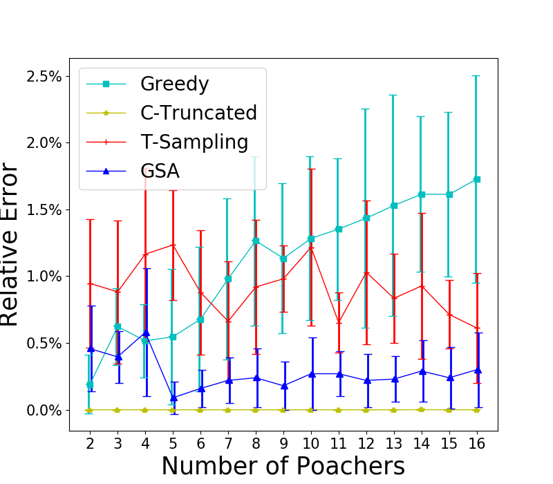
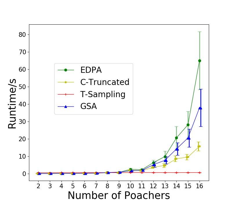
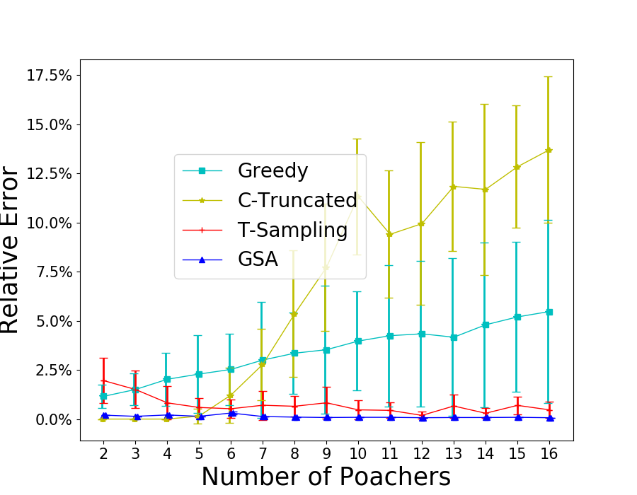
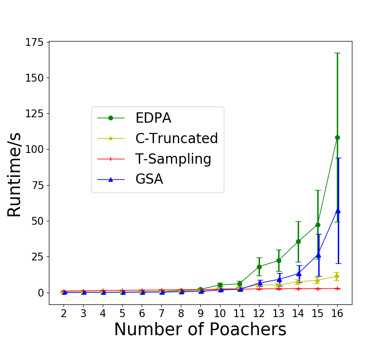
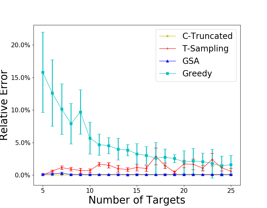
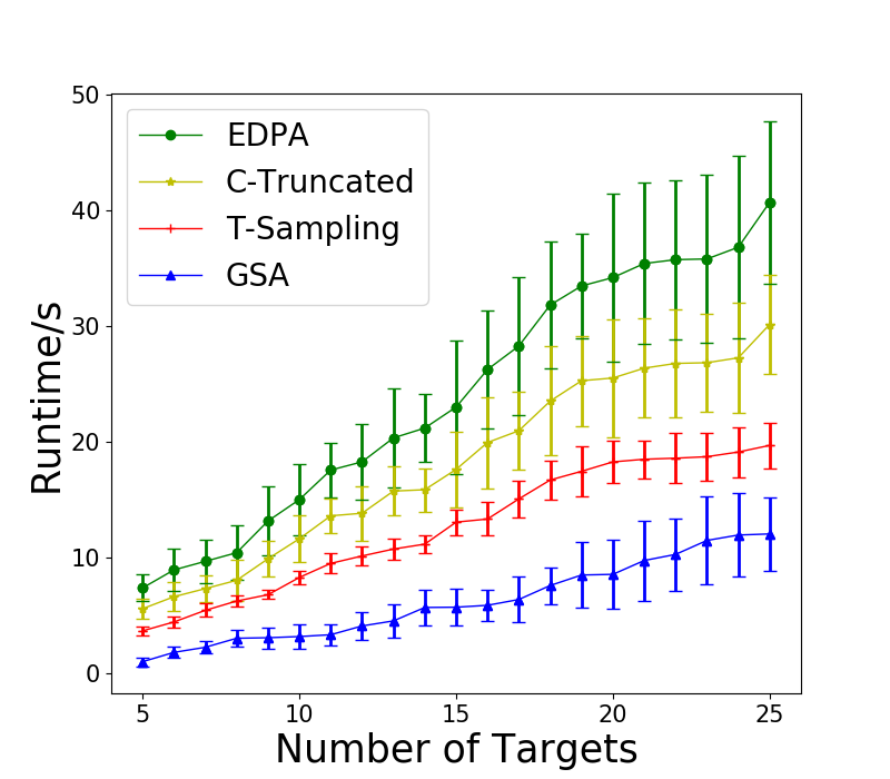
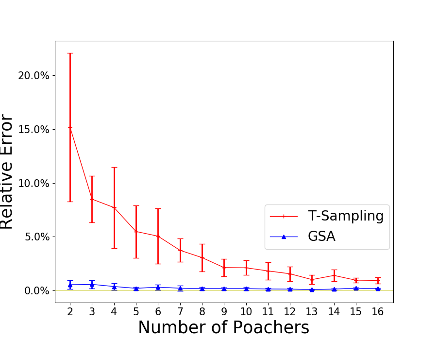
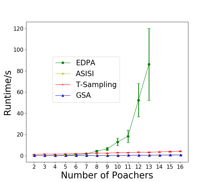
First, we test the case where . We set and enumerate from 2 to 16. The results are shown in Figure 1(a). We also include Greedy as a baseline that always chooses the informants that maximizes the probability of receiving tips. We can see that T-Sampling performs the best in term of runtime, but fails to provide high-quality solutions. While C-Truncated is slower than T-Sampling, it performs the best with no error on all test cases. However, when there is no restriction on , as shown in Figure 1(b), C-Truncated performs badly, even worse than Greedy for large , while T-Sampling performs a lot better and GSA performs the best. We also fix , and change the number of targets from 5 to 25 for . The results are shown in Figure 1(c). GSA is the fastest but provides slightly worse solutions than C-Truncated does. The runtime of Greedy is less than 0.3s for all instances tested.
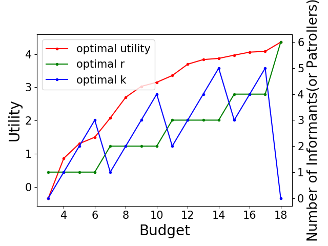
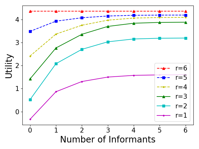
We then perform a case study to show the trade-off between the optimal number of resources to allocate and the optimal number of informants to recruit with budget constraints when defending against level-0 attackers. We set and generate an instance of the game. We set the cost of allocating one defensive resource and the cost of hiring one informant . Given a budget , we can recruit informants and allocate resources when . The trade-off between the optimal and is shown in Figure 1(d). In the same instance, we study how the defender’s utility would change by increasing the number of recruited informants with fixed . Given a fixed number of resources, the defender should recruit as many informants as possible. We can also see that assuming the defender can acquire sufficient resources, the importance of recruiting additional informants is diminished. This result provides useful guidance to defenders such as conservation agencies in allocating their budget and recruiting informants.
We run additional experiments for the SISI case and do a case study to show the errors of the estimations for all on 2 instances. We present the results in Appendix K.
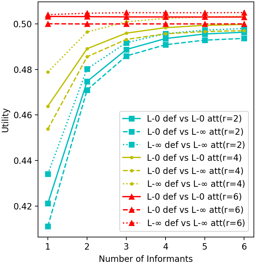
7.1.1. Level-0 vs. Level- attackers
We set , , and to be fully connected. We set and vary from . We first fix the defender’s strategy to the one against level-0 attackers and compare the utility achieved by the defender when defending against a level-0 attacker and a level- attacker. We show how the defender utility varies with the number of informants and defensive resources in Figure 1(e). On average, we see that the defender utility against a level- attacker is lower than that against a level-0 attacker. We also show the utility of the defender using her optimal strategy against a level- attacker. We can see that when facing a level- attacker, the defender utility when using the optimal strategy is higher by a margin than using the one against level-0 attackers.
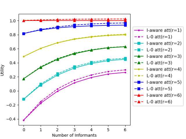
7.1.2. Level-0 vs. informant-aware defenders
We set , , and to be fully connected. We vary from and from . We assume that the defender recruits the informants with the highest information sharing intensity . The optimal defender strategy against the informant-aware attacker case is found using QRI-MILP. The defender strategy against the level-0 attacker case is computed using PASAQ Yang et al. (2012). The defender utility against the level-0 attacker is found by first computing and then using the results to compute .
In Figure 1(g), we show how the defender utility in the two cases varies with the number of informants and defensive resources. On average, we see that the defender utility is marginally higher against the level-0 attacker than against the informant-aware attacker, particularly when the defender has either very few or very many defensive resources. We also compare the defender’s utility of the level-0 defender (defending against level-0 attackers) and the informant-aware defender (defending against informant-aware attackers). The results are deferred to Appendix K.
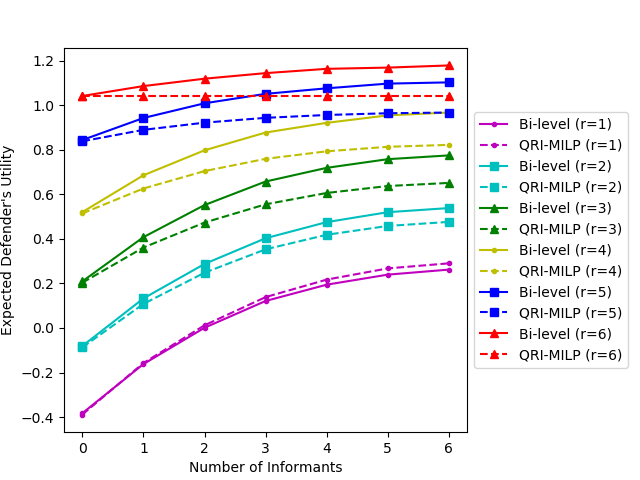
7.1.3. Comparison between the Bi-Level Algorithm and QRI-MILP
We empirically compare the bi-level optimization algorithm with QRI-MILP. We set , , and to be fully connected. We vary from and from .
In both cases, we assume that the defender recruits the informants with the highest information sharing intensity . The results are shown in Figure 1(f). In general, our bi-level algorithm gives higher expected defender utilities than the QRI-MILP algorithm, except when . Our results show that both increasing the number of resources and hiring more informants increase the defender’s utility. However, as the number of resources () increases, the utility gain from hiring more informants diminishes.
Intuitively, if the number of resources equals the number of targets, the defender should always cover all the targets, Interestingly, during our experiments, we observed that in this case, the optimal defender strategy may not always use all his resources to cover all the targets. The reason is that in a general sum game, by decreasing the probability of protecting a certain target on purpose, the defender can lure the attacker into attacking the target more frequently, and thus increase his expected utility. Such strategies can be found in real-world wildlife protections where the patrollers may sometimes deliberately ignore the tips. This is also reflected in our bi-level algorithm. If the defender always uses all his resources, then both the defender’s and the attacker’s strategies are fixed, and hiring more informants does not increase the defender’s expected utility. But if the defender strategy does not always use all his resources, then hiring more informants could help (see the bi-level algorithm for the case in Figure 1(f)).
8. Discussion and Conclusion
In this paper, we introduced a novel two-stage security game model and a multi-level QR behavioral model that incorporated community engagement. We provided complexity results, developed algorithms to find (sub-)optimal groups of informants to recruit against level-0 attackers and evaluated the algorithms through extensive experiments. Our results also generalize to the case where informants have heterogeneous recruitment costs and to different kinds of attacker response models, such as SUQR model Nguyen et al. (2013), which can be done by calculating the attacker’s response correspondingly. Also, see Appendix M on how to extend our algorithms to defend against level- () attackers. In Section 5, we defined a more powerful type of attacker that could respond to the marginal strategy and developed a bi-level optimization algorithm to find the optimal defender’s strategy in this case.
In the anti-poaching domain, some conservation site managers utilize the so-called “intelligence” operations that rely on informants in nearby villages to alert rangers when they know the poachers’ plans in advance. The deployment of the work relies on the site manager to provide their understanding of the social connections among community members. The edges and parameters of the bipartite graph in our model can be extracted from a local social media application or historical data collected by site managers. Recruiting and training reliable informants is costly and managers may only afford a limited number of them. Our model and solution can help the managers efficiently recruit informants, make the best use of tips and evaluate the trade-off between allocating budget to hiring rangers and recruiting informants in a timely fashion.
For future work, instead of using a particular behavior model, we can use historical records as training data and learn the attackers’ behavior in different domains. It would also be interesting to consider the case where the informants can only provide inaccurate tips or other types of tips, e.g., some subset of targets will be attacked instead of a single location. We can also model the informants as strategic agents. In real life, it is possible that informants may also provide fake information if they have their own utility structures. We can try to reward them to elicit true information and maximize the defender’s utility.
Acknowledgement
This work is supported in part by NSF grant IIS-1850477 and a research grant from Lockheed Martin.
References
- (1)
- Basilico et al. (2017) Nicola Basilico, Andrea Celli, Giuseppe De Nittis, and Nicola Gatti. 2017. Coordinating multiple defensive resources in patrolling games with alarm systems. In AAMAS’17. 678–686.
- Duffy et al. (2015) Rosaleen Duffy, Freya AV St John, Bram Büscher, and DAN Brockington. 2015. The militarization of anti-poaching: undermining long term goals? Environmental Conservation 42, 4 (2015), 345–348.
- Fang et al. (2017) Fei Fang, Thanh Hong Nguyen, Rob Pickles, Wai Y. Lam, Gopalasamy R. Clements, Bo An, Amandeep Singh, Brian C. Schwedock, Milind Tambe, and Andrew Lemieux. 2017. PAWS - A Deployed Game-Theoretic Application to Combat Poaching. AI Magazine (2017). http://www.aaai.org/ojs/index.php/aimagazine/article/view/2710
- Gill et al. (2014) Charlotte Gill, David Weisburd, Cody W Telep, and Trevor Bennett. 2014. Community-oriented policing to reduce crime, disorder and fear and increase satisfaction and legitimacy among citizens: A systematic review. Journal of Experimental Criminology (2014).
- Guo et al. (2017) Qingyu Guo, Boyuan An, Branislav Bosansky, and Christopher Kiekintveld. 2017. Comparing strategic secrecy and Stackelberg commitment in security games. In IJCAI-17.
- Jain et al. (2010) Manish Jain, Jason Tsai, James Pita, Christopher Kiekintveld, Shyamsunder Rathi, Milind Tambe, and Fernando Ordónez. 2010. Software assistants for randomized patrol planning for the lax airport police and the federal air marshal service. Interfaces (2010).
- Korzhyk et al. (2011) Dmytro Korzhyk, Zhengyu Yin, Christopher Kiekintveld, Vincent Conitzer, and Milind Tambe. 2011. Stackelberg vs. Nash in security games: An extended investigation of interchangeability, equivalence, and uniqueness. Journal of Artificial Intelligence Research 41 (2011), 297–327.
- Le Gallic and Cox (2006) Bertrand Le Gallic and Anthony Cox. 2006. An economic analysis of illegal, unreported and unregulated (IUU) fishing: Key drivers and possible solutions. Marine Policy 30, 6 (2006), 689–695.
- Leader-Williams and Milner-Gulland (1993) N Leader-Williams and EJ Milner-Gulland. 1993. Policies for the enforcement of wildlife laws: the balance between detection and penalties in Luangwa Valley, Zambia. Conservation Biology 7, 3 (1993), 611–617.
- Linkie et al. (2015) Matthew Linkie, Deborah J. Martyr, Abishek Harihar, Dian Risdianto, Rudijanta T. Nugraha, Maryati, Nigel Leader‐Williams, and Wai‐Ming Wong. 2015. EDITOR’S CHOICE: Safeguarding Sumatran tigers: evaluating effectiveness of law enforcement patrols and local informant networks. Journal of Applied Ecology (2015).
- Ma et al. (2018) Xiaobo Ma, Yihui He, Xiapu Luo, Jianfeng Li, Mengchen Zhao, Bo An, and Xiaohong Guan. 2018. Camera Placement Based on Vehicle Traffic for Better City Security Surveillance. IEEE Intelligent Systems 33, 4 (Jul 2018), 49–61. https://doi.org/10.1109/mis.2018.223110904
- McKelvey and Palfrey (1995) Richard D McKelvey and Thomas R Palfrey. 1995. Quantal response equilibria for normal form games. Games and economic behavior (1995).
- Moreto (2015) William D Moreto. 2015. Introducing intelligence-led conservation: bridging crime and conservation science. Crime Science 4, 1 (2015), 15.
- Nemhauser et al. (1978) George L Nemhauser, Laurence A Wolsey, and Marshall L Fisher. 1978. An analysis of approximations for maximizing submodular set functions—I. Mathematical programming 14, 1 (1978), 265–294.
- Nguyen et al. (2013) Thanh Hong Nguyen, Rong Yang, Amos Azaria, Sarit Kraus, and Milind Tambe. 2013. Analyzing the Effectiveness of Adversary Modeling in Security Games.. In AAAI.
- Pita et al. (2008) James Pita, Manish Jain, Janusz Marecki, Fernando Ordóñez, Christopher Portway, Milind Tambe, Craig Western, Praveen Paruchuri, and Sarit Kraus. 2008. Deployed ARMOR protection: the application of a game theoretic model for security at the Los Angeles International Airport. In AAMAS: industrial track.
- Rosenfeld and Kraus (2017) Ariel Rosenfeld and Sarit Kraus. 2017. When Security Games Hit Traffic: Optimal Traffic Enforcement Under One Sided Uncertainty.. In IJCAI. 3814–3822.
- Schlenker et al. (2018) Aaron Schlenker, Omkar Thakoor, Haifeng Xu, Fei Fang, Milind Tambe, Long Tran-Thanh, Phebe Vayanos, and Yevgeniy Vorobeychik. 2018. Deceiving Cyber Adversaries: A Game Theoretic Approach. In AAMAS.
- Short et al. (2013) Martin B Short, Ashley B Pitcher, and Maria R D’Orsogna. 2013. External conversions of player strategy in an evolutionary game: A cost-benefit analysis through optimal control. European Journal of Applied Mathematics 24, 1 (2013), 131–159.
- Smith and Humphreys (2015) MLR Smith and Jasper Humphreys. 2015. The Poaching Paradox: Why South Africa’s ‘Rhino Wars’ Shine a Harsh Spotlight on Security and Conservation. Ashgate Publishing Company.
- Tambe (2011) Milind Tambe. 2011. Security and game theory: algorithms, deployed systems, lessons learned. Cambridge University Press.
- Tublitz and Lawrence (2014) Rebecca Tublitz and Sarah Lawrence. 2014. The Fitness Improvement Training Zone Program. (2014).
- Wang et al. (2018) Xinrun Wang, Bo An, Martin Strobel, and Fookwai Kong. 2018. Catching Captain Jack: Efficient Time and Space Dependent Patrols to Combat Oil-Siphoning in International Waters. (2018). https://www.aaai.org/ocs/index.php/AAAI/AAAI18/paper/view/16312
- Wright and Leyton-Brown (2014) James R Wright and Kevin Leyton-Brown. 2014. Level-0 meta-models for predicting human behavior in games. In Proceedings of the fifteenth ACM conference on Economics and computation. ACM, 857–874.
- WWF (2015) WWF. 2015. Developing an approach to community-based crime prevention. http://zeropoaching.org/pdfs/Community-based-crime%20prevention-strategies.pdf. (2015).
- Yang et al. (2012) Rong Yang, Fernando Ordonez, and Milind Tambe. 2012. Computing optimal strategy against quantal response in security games. In AAMAS.
Appendix:
Green Security Game with Community Engagement
Appendix A Complexity of different algorithms
| Algorithm | Time Complexity |
|---|---|
| EDPA | |
| C-Truncated | |
| T-Sampling | |
| ASISI | |
| GSA |
Appendix B Proof of Theorem 4.1
See 4.1
Proof.
Given the tips , the defender should calculate for each target , and then allocate the resources to of the targets with the highest .
The above strategy is indeed optimal since the expected utility with no resources is given by , and once an additional unit of resource is given, it should always be allocated to the uncovered target that could lead to the largest increment in expected utility, i.e., the target with the largest .
The calculation of for each can be done in time, and finding the largest can be done in time, leading to the overall complexity of . ∎
Appendix C Proof of Theorem 4.1
See 4.1
Proof.
Consider the case where , for all , and the targets are uniform i.e., ’s () are the same for all . We use the notation () instead of () for simplicity. Let .
To start with, we investigate how depends on a given . Since and for all , all attackers in will be reported to attack a location. Let random variable be the number of attackers who are reported to attack location . Since the targets are uniform, an attacker will attack each location with probability if he goes attacking. Then the defender’s expected utility could be written as
The latter two terms are independent of the choice of informants so to maximize , it suffices the maximize .
We can prove by induction on that increases as increases, or increases by at least if is increased by 1:
-
(1)
Since when and when , it holds for .
-
(2)
Consider and the corresponding sequence . Let . We add an attacker to and denote by the probability of he targeting the location with the largest . Thus the expected maximum increase by . Since and by a simple coupling argument, we have that increases by at least
Thus, in this case, solving for the optimal solution of the original problem is equivalent to solving for that maximizes the size of in the first stage.
We show that the optimization problem is NP-Hard using a reduction from : we are given a number and a collection of sets . The objective is to find a subset of sets such that and the number of covered elements is maximized. Let , , , for all and for all . Thus to find a with that maximizes the size of is equivalent to finding a subset of sets with size no larger than that maximizes the number of covered elements in the instance of . ∎
Appendix D Proof of Lemma 4.2.2
See 4.2.2
Proof.
Since for all , we have for each given . Therefore, the expected gain of target with reported attacks can be written as and the calculation of depends only on the size of . Thus, instead of enumerating , we enumerate as the size of in line 2 of Algorithm 1, and replace in Algorithm 1 with , where can be obtained by expanding the following polynomial Therefore, can be calculated in time.
Since all possible can be enumerated in , the optimal set of informants can be computed in . ∎
Appendix E ASISI
Appendix F Defender Utility is not Submodular
We provide a counterexample that disproves the submodularity of .
Example \thetheorem
Consider a network where , , , and . There are 2 targets , where , for any . Letting yields . The defender has only 1 resource. We can see that , As a result,
Appendix G Proof of Lemma 4.2.1
See 4.2.1
Proof.
Let the random variable be the number of attacks. Let be the set of events of having no less than reported attackers and be the set of events of having no less than attacks. Let be the expected defender’s utility taken over all possible tips given an event . By noticing that , we have
| (6) | |||||
| (7) |
Inequality (6) follows by the Chernoff Bound, and inequality (7) follows since
∎
Appendix H Non-convergence of the level- response
Example \thetheorem
Suppose there is a single attacker and two targets with the following payoffs:
In this case, there are only two possible tips: the attacker attacks target 1 (), and the attacker attacks 2 (). Assume that only 1 informant is recruited with report probability . The defender has only 1 defensive resource and uses the following strategy:
When the attacker has , the level- response will converge to . However, if , then the process will eventually oscillate between and iteratively.
Appendix I Proof of Lemma 5.1
See 5.1
Proof.
Given defender’s strategy and , define:
Then a level-(+1) attacker’s strategy can be computed by
The convergence of level- is equivalent to the convergence of .
The marginal strategy can be written as:
Notice that the function is just the quantal response against :
where is the attacker’s expected utility of attacking target when the defender’s marginal strategy is : . Therefore,
Note that in the above equation, , and . Thus we have:
| (8) |
On the other hand, means . Plugging into Equation (8), we get:
For any , let . So and . Therefore,
∎
Appendix J Algorithm for Defending against Informant-Aware Attackers
Proposition \thetheorem
The optimal objective of QRI is non-decreasing in .
Proof.
Consider the two optimization problems induced by different values for : where . Let be a solution for when . Then, is a feasible solution for when that achieves the same objective value. To see why it is feasible, observe that constraint (3) is satisfied by construction and constraint (5) is satisfied since the new value for each is a convex combination of the previous , which were both in . ∎
Proposition J implies that when selecting informants, it is optimal to simply maximize . Since , we can select informants greedily and choose the informants with the largest information sharing intensity . We can then solve the optimization problem to find the optimal allocation of resources. Finally, we discuss how to find an approximate solution to QRI using a MILP approach.
We can compute the optimal defender strategy by adapting the approach used in the PASAQ algorithm Yang et al. (2012). Let be the numerator and denominator of the objective in QRI. As with PASAQ, we binary search on the optimal value . We can check for feasibility of a given by rewriting the objective to and checking if the optimal value is less than . To solve the new optimization problem, which still has a non-linear objective function, we adapt their approach of approximating the objective function with linear constraints and write a MILP.
First, let , , and . We rewrite the objective as
We have two non-linear functions that need approximation and . Let be the slope for the linear approximation of from to and similarly with for .
The key change in our MILP compared to PASAQ is that we replace the original defender resource constraint with constraints (9) - (12), which take into account the ability of the defender to respond to tips.
QRI-MILP:
| subject to | (9) | |||
| (10) | ||||
| (11) | ||||
| (12) | ||||
| (13) | ||||
| (14) | ||||
| (15) | ||||
| (16) |
Proposition \thetheorem
The feasible region for of QRI-MILP is equivalent to that of QRI.
Proof.
With the above claim shown, the proof for the approximate correctness of PASAQ applies here and we can show that we can find an -optimal solution for arbitrarily small Yang et al. (2012).
Appendix K Additional Experiment Results
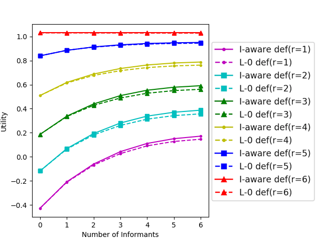
In Figure 2, we compare the performance of the level-0 defender and the informant-aware defender when playing against an informant-aware attacker. We see that despite that their strategies are computed under the level-0 attacker assumption, the utility of the level-0 defender is only slightly lower than the utility of the informant-aware defender. For a fixed , the difference in utility grows larger as the defender recruits more informants and has a higher probability of receiving a tip.
We test the special case assuming SISI. We set and enumerate from 2 to 16. The average runtime of all algorithms including ASISI together with the relative error of GSA and T-Sampling are shown in Figure 3. Though ASISI and GSA are the fastest among all, the average relative errors of GSA are slightly above . T-Sampling is slightly slower than ASISI and GSA, and the solutions are less accurate than the other two in this case.
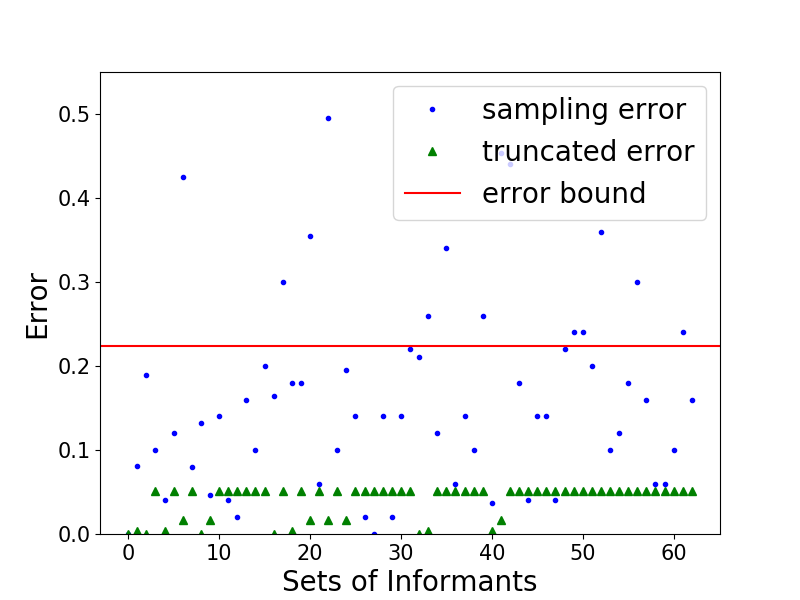
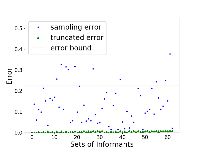
Another experiment is a case study on 2 instances with fixed , , , , . We run EDPA, C-Truncated () and T-Sampling on each instance and show the error of the estimations for all . The results are shown in Figure 4 and the red lines indicate the error bound given by Lemma 4.2.1. We encode the set of informants in binary, e.g., the set with code represents the set The first instance is constructed to show that the bound given by Lemma 4.2.1 is empirically tight, i.e., the estimation of by C-Truncated could be large but still bounded. In this case, we set , and While the other instance is randomly generated. It is shown that T-Sampling has larger errors with higher variances compared to C-Truncated.
Appendix L Experiment Setup
To generate , we first fix the sets and . For each , we sample the degree of , , uniformly from and then sample a uniformly random subset of of size . For each , is drawn from . For the attack probability , in the general case, each is drawn from . When we restrict , we draw a vector from and set }. For the payoff matrix, each () is drawn from and each is drawn from , where is set to 2. The precision parameter is set to 2. and ’s are obtained by a binary search with a convex optimization as introduced in Yang et al. (2012). The number of samples used in T-Sampling is set to 100. In GSA, EDPA is used to calculate .
In the QRI-MILP algorithm, the optimal defender strategy is found with approximation parameter . The bi-level optimization algorithm is implemented using MATLAB R2017a. The low-level linear program is solved using the linprog function and the high-level optimization is solved with the fmincon function.
Appendix M Defending Against Level- Attackers
In the section 4, we deal with the case with only type-0 attackers and provide algorithms to find the optimal set of informants to recruit. In this section, we show how those approaches can be easily extended to the case with level- attackers.
Once given , can be easily obtained. So as , the defender’s expected utility using against a single attack of a level- attacker. To get the solution, we simply replace with and apply Select or GSA. In order to calculate by definition, all that remains is to calculate for . The marginal probability of each target being covered can be calculated in a way similar to EDPA.