Université Libre de Bruxelles, Belgiumanirban.majumdar@ulb.behttps://orcid.org/0000-0003-4793-1892funded by a grant from Fondation ULB Université Libre de Bruxelles, Belgiumsayan.mukherjee@ulb.behttps://orcid.org/0000-0001-6473-3172funded by a grant from Fondation ULB Université Libre de Bruxelles, Belgiumjean-francois.raskin@ulb.behttps://orcid.org/0000-0002-3673-1097receives support from the Fondation ULB \ccsdescTheory of computation Timed and hybrid models \supplementThe source codes related to our algorithm can be found as follows: \supplementdetails[subcategory=Source Code]Softwarehttps://github.com/mukherjee-sayan/ERA-greybox-learn \supplementdetails[subcategory=]ATVA 2024 Artifact Evaluation approved artifacthttps://doi.org/10.5281/zenodo.12684215 \hideLIPIcs
Greybox Learning of Languages Recognizable by Event-Recording Automata
Abstract
In this paper, we revisit the active learning of timed languages recognizable by event-recording automata. Our framework employs a method known as greybox learning, which enables the learning of event-recording automata with a minimal number of control states. This approach avoids learning the region automaton associated with the language, contrasting with existing methods. We have implemented our greybox learning algorithm with various heuristics to maintain low computational complexity. The efficacy of our approach is demonstrated through several examples.
keywords:
Automata learning, Greybox learning, Event-recording automata1 Introduction
Formal modeling of complex systems is essential in fields such as requirement engineering and computer-aided verification. However, the task of writing formal models is both laborious and susceptible to errors. This process can be facilitated by learning algorithms [21]. For example, if a system can be represented as a finite state automaton, and thus if the system’s set of behaviors constitutes a regular language, there exist thoroughly understood passive and active learning algorithms capable of learning the minimal DFA of the underlying language111Minimal DFAs are a canonical representation of regular languages and are closely tied to the Myhill-Nerode equivalence relation. We call this problem the specification discovery problem in the sequel. In the realm of active learning, the algorithm [5], pioneered by Angluin, is a celebrated approach that employs a protocol involving membership and equivalence queries, and enabling an efficient learning process for regular languages.
In this paper, we introduce an active learning framework designed to acquire timed languages that can be recognized by event-recording automata (ERA, for short)[3]. The class of ERA enjoys several nice properties over the more general class of Timed Automata (TA) [2]. First, ERA are determinizable and hence complementable, unlike TA, making it particularly well suited for verification as inclusion checking is decidable for this class. Second, in ERA, clocks are explicitly associated to events and implicitly reset whenever its associated event occurs. This property leads to automata that are usually much easier to interpret than classical TA where clocks are not tied to events. This makes the class of ERA a very interesting candidate for learning, when interpretability is of concern.
Adapting the algorithm for ERA is feasible by employing a canonical form known as the simple deterministic event-recording automata (SDERA). These SDERAs, introduced in [12] specifically for this application, are essentially the underlying region automaton of the timed language. Although the region automaton fulfills all the necessary criteria for the algorithm, its size is generally excessive. Typically, the region automaton is significantly larger than a deterministic ERA (DERA, for short) with the minimum number of locations for a given timed language (and it is known that it can be exponentially larger). This discrepancy arises because the region automaton explicitly incorporates the semantics of clocks in its states, whereas in a DERA, the semantics of clocks are implicitly utilized. The difficulty to work directly with DERA is related to the fact that there is no natural canonical form for DERA and usually, there are several DERA with minimum number of states that recognize the same timed language. To overcome this difficulty, we propose in this paper an innovative application of the greybox learning framework, see for example [1], and demonstrate that it is possible to learn an automaton whose number of states matches that of a minimum DERA for the underlying timed language.
In our approach, rather than learning the region automaton of the timed language, we establish an active learning setup in which the semantics of the regions are already known to the learning algorithm, thus eliminating the need for the algorithm to learn the semantics of regions. Our greybox learning algorithm is underpinned by the following concept:
| (1) |
Here, is a set of consistent region words that exactly represents the target timed language . Meanwhile, denotes the regular language of consistent region words across the alphabet and a maximal constant . This language is precisely defined once and are fixed and remains independent of the timed language to be learned; therefore, it does not require learning. Essentially, deciding if a region word belongs to or not reduces to solving the following “consistency problem”: given a region word, are there concrete timed words consistent with this (symbolic) region word? The answer to this question does not depend on the timed language to be learned but only on the semantics of clocks. This reduces the consistency problem to the problem of solving a linear program, which is known to be solvable efficiently.
The target of our greybox learning algorithm is a DERA recognizing the timed language . We will demonstrate that if a DERA with states can accept the timed language to be learned, then the DERA returned by our algorithm has at most many states. Here is an informal summary of our learning protocol: within the context of the vocabulary, we assume that the Teacher is capable of responding to membership queries of consistent region words. Additionally, the Teacher handles inclusion queries, unlike equivalence queries in by determining whether a timed language is contained in another. If a discrepancy exists, Teacher provides a counter-example in the form of a region word.
This learning framework can be applied to specification discovery problem presented in the motivations above: we assume that the requirements engineer has a specific timed language in mind for which he wants to construct a DERA, but we assume that he is not able to formally write this DERA on his own. However, the requirement engineer is capable of answering membership and inclusion queries related to this language. Since the engineer cannot directly draft a DERA that represents the timed language, it is crucial that the queries posed are semantic, focusing on the language itself rather than on a specific automaton representing the language. This distinction ensures that the questions are appropriate and manageable given the assumptions about the engineer’s capabilities. This is in contrast with [15], where queries are syntactic and answered with a specific DERA known by the Teacher. We will give more details about this comparison later in Section 3.
Technical contribution.
First, we define a greybox learning algorithm to derive a DERA with the minimal number of states that recognizes a target timed language. To achieve the learning of a minimal automaton, we must solve an NP-hard optimization problem: calculating a minimal finite state automaton that separates regular languages of positive and negative examples derived from membership and equivalence queries [11]. For that, we adapt to the timed setting the approach of Chen et al. in [7]. A similar framework has also been studied using SMT-based techniques by Moeller et al. in [16]. Second, we explore methods to circumvent this NP-hard optimization problem when the requirement for minimality is loosened. We introduce a heuristic that computes a candidate automaton in polynomial time using a greedy algorithm. This algorithm strives to maintain a small automaton size but does not guarantee the discovery of the absolute minimal solution, yet guaranteed to terminate with a DERA that accepts the input timed language. We have implemented this heuristic and demonstrate with our prototype that, in practice, it yields compact automata.
Related works.
Grinchtein et al. in [12] also present an active learning framework for ERA-recognizable languages. However, their learning algorithm generates simple DERAs – these are a canonical form of ERA recognizable languages, closely aligned with the underlying region automaton. In a simple DERA, transitions are labeled with region constraints, and notably, every path leading to an accepting state is satisfiable. This means the sequence of regions is consistent (as in the region automaton), and any two path prefixes reaching the same state are region equivalent. Typically, this results in a prohibitively large number of states in the automaton that maintains explicitly the semantics of regions. In contrast, our approach, while also labeling automaton edges with region constraints, permits the merging of prefixes that are not region equivalent. Enabled by equation 1, this allows for a more compact representation of the ERA languages (we generate DERA with minimal number of states). While our algorithm has been implemented, there is, to the best of our knowledge, no implementation of Grinchtein’s algorithm, certainly due to high complexity of their approach.
Lin et al. in [15] propose another active learning style algorithm for inferring ERA, but with zones (coarser constraints than regions) as guards on the transitions. This allows them to infer smaller automata than [12]. However, it assumes that Teacher is familiar with a specific DERA for the underlying language and is capable of answering syntactic queries about this DERA. In fact, their learning algorithm is recognizing the regular language of words over the alphabet, composed of events and zones of the specific DERA known to Teacher. Unlike this approach, our learning algorithm does not presuppose a known and fixed DERA but only relies on queries that are semantic rather than syntactic. Although the work of [15] may seem superficially similar to ours, we dedicate in Section 3 an entire paragraph to the formal and thorough comparison between our two different approaches.
Recently, Masaki Waga developed an algorithm [24] for learning the class of Deterministic Timed Automata (DTA), which includes ERA recognizable languages. Waga’s method resets a clock on every transition and utilizes region-based guards, often producing complex automata. Consequently, this algorithm does not guarantee the minimality of the resulting automaton, but merely ensures it accepts the specified timed language. In contrast, our approach guarantees learning of automata with the minimal number of states, featuring implicit clock resets that enhance readability. In the experimental section, we detail a performance comparison of our tool against their tool, LearnTA, across various examples. Further, in [20], the authors extend Waga’s approach to reduce the number of clocks in learned automata, though they also do not achieve minimality. Their method also requires a significantly higher number of queries to implement these improvements.
Several other works have proposed learning methods for different models of timed languages, such as, One-clock Timed Automata [25], Real-time Automata [4], Mealy-machines with timers [22, 6]. There have also been approaches other than active learning for learning such models, for example, using Genetic programming [19] and passive learning [23, 8].
2 Preliminaries and notations
DFA and 3DFA.
Let be a finite alphabet. A deterministic finite state automaton (DFA) over is a tuple where is a finite set of states, is the initial state, is a partial transition function, and is the set of final (accepting) states. When is a total function, we say that is total. A DFA defines a regular language, noted , which is a subset of and which contains the set of words such that there exists an accepting run of over , i.e., there exists a sequence of states such that , and for all , , , and . We then say that the word is accepted by . If such an accepting run does not exist, we say that rejects the word .
A 3DFA over is a tuple where is a finite set of states, is the initial state, is a total transition function, and forms a partition of into a set of accepting states , a set of rejection states , and a set of ‘don’t care’ states . The 3DFA defines the function as follows: for let be the unique run of on . If (resp. ), then (resp. ) and we say that is strongly accepted (resp. strongly rejected) by , and if , then . We interpret “” as either way, i.e., so the word can be either accepted or rejected. We say that a regular language is consistent with a 3DFA , noted , if for all , if then , and if then . Accordingly, we define as the DFA obtained from where the partition is replaced by , clearly , it is thus the set of words that are strongly rejected by . Similarly, we define as the DFA obtained from where the partition is replaced by , then , it is thus the set of words that are strongly accepted by . Now, it is easy to see that iff and .
Timed words and timed languages.
A timed word over an alphabet is a finite sequence where each and , for all , and for all , (time is monotonically increasing). We use to denote the set of all timed words over the alphabet .
A timed language is a (possibly infinite) set of timed words. In existing literature, a timed language is called timed regular when there exists a timed automaton ‘recognizing’ the language. Timed Automata (TA) [2] extend deterministic finite-state automata with clocks. In what follows, we will use a subclass of TA, where clocks have a pre-assigned semantics and are not reset arbitrarily. This class is known as the class of Event-recording Automata (ERA) [3]. We now introduce the necessary vocabulary and notations for their definition.
Constraints.
A clock is a non-negative real valued variable, that is, a variable ranging over . Let be a positive integer. An atomic -constraint over a clock , is an expression of the form , or where . A -constraint over a set of clocks is a conjunction of atomic -constraints over clocks in . Note that, -constraints are closely related to the notion of zones [10] as in the literature of TA. However, zones also allow difference between two clocks, that are not allowed in -constraints.
An elementary -constraint over a clock , is an atomic -constraint where the intervals are restricted to unit intervals; more formally, it is an expression of the form , or where . A simple -constraint over is a conjunction of elementary -constraints over clocks in , where each variable appears exactly in one conjunct. The definition of simple constraints also appear in earlier works, for example [12]. One can again note that, simple constraints closely relate to the classical notion of regions [2]. However, again, regions consider difference between two clocks as well, which simple constraints do not. Interestingly, we do not need the granularity that regions offer (by comparing clocks) for our purpose, because a sequence of simple constraints induce a unique region in the classical sense (see Lemma 2.6).
Satisfaction of constraints.
A valuation for a set of clocks is a function . A valuation for satisfies an atomic -constraint , written as , if: when , when and when .
A valuation satisfies a -constraint over if satisfies all its conjuncts. Given a -constraint , we denote by the set of all valuations such that . We say that a simple constraint satisfies an elementary constraint , noted , if . It is easy to verify that for any simple constraint and any elementary constraint , either or .
Let be a finite alphabet. The set of event-recording clocks associated to is denoted by . We denote by the set of all -constraints over the set of clocks and we use to denote the set of all simple -constraints over the clocks in . For simple -constraints we adopt the notation , since, as remarked earlier, these kinds of constraints relate closely to the well-known notion of regions. Since simple -constraints are also -constraints, we have that .
Definition 2.1 (ERA).
A -Event-Recording Automaton (-ERA) is a tuple where is a finite set of states, is the initial state, is a finite alphabet, is the set of transitions, and is the subset of accepting states. Each transition in is a tuple , where , and , is called the guard of the transition. is called a -deterministic-ERA (-DERA) if for every state and every letter , if there exist two transitions and then .
For the semantics, initially, all the clocks start with the value and then they all elapse at the same rate. For every transition on a letter , once the transition is taken, its corresponding recording clock gets reset to the value .
Clocked words.
Given a timed word , we associate with it a clocked word where each maps each clock of to a real-value as follows: where , with the convention that . In words, the value is the amount of time elapsed since the last occurrence of in tw; which is why we call the clocks ‘recording’ clocks. Although not explicitly, clocks are implicitly reset after every occurrence of their associated events.
Timed language of a -ERA.
A timed word with its clocked word , is accepted by if there exists a sequence of states of such that , , and for all , there exists such that , and . The set of all timed words accepted by is called the timed language of , and will be denoted by . We now ask a curious reader: is it possible to construct an ERA with two (or less) states that accepts the timed language represented in Figure 1? We will answer this question in Section 5.
Lemma 2.2 ([3]).
For every -ERA , there exists a -DERA such that and there exists a -DERA such that .
A timed language is -ERA (resp. -DERA) definable if there exists a -ERA (resp. -DERA) such that . Now, due to Lemma 2.2, a timed language is -ERA definable iff it is -DERA definable.
Symbolic words
over are finite sequences where each and , for all . Similarly, a region word over is a finite sequence where each and is a simple -constraint, for all . Lemma 2.6 will justify why we refer to symbolic words over simple constraints as ‘region’ words.
We are now equipped to define when a timed word is compatible with a symbolic word . Let be a timed word with its clocked word being , and let be a symbolic word. We say that is compatible with , noted , if we have that: , i.e., both words have the same length, and , for all , . We denote by . We say that a symbolic word is consistent if , and inconsistent otherwise. We will use to denote the set of all consistent region words over the set of all -simple constraints .
Example 2.3.
Let be an alphabet and let be its set of recording clocks. The symbolic word is consistent, since the timed word . On the other hand, consider the symbolic word . Let be a timed word and be the clocked word of . Then would imply and , but in that case, , that is, . Hence, is inconsistent.
Lemma 2.4.
For every timed word over an alphabet , for every fixed positive integer , there exists a unique region word where .
Proof 2.5 (Proof sketch).
Given a timed word , consider its clocked word (as in Page 2). Now, it is easy to see that each clock valuation satisfies only one simple -constraint. Therefore, we can construct a region word by replacing the valuations present in with the simple -constraints they satisfy, thereby constructing the (unique) region word that is compatible with.
Lemma 2.6.
For every -ERA over an alphabet and for every region word , either or . Equivalently, for all timed words , iff .
The above lemma states that, two timed words that are both compatible with one region word, cannot be ‘distinguished’ using a DERA. This can be proved using Lemma of [12].
Symbolic languages.
Note that, every -DERA can be transformed into another -DERA where every guard present in is a simple -constraint. This can be constructed as follows: for every transition in where is a -constraint (and not a simple -constraint), contains the transitions such that . Since, for every -constraint , there are only finitely-many (possibly, exponentially many) simple -constraints that satisfy , this construction indeed yields a finite automaton. As for an example, the transition from to in the automaton in Figure 1 contains a non-simple -constraint as guard. This transition can be replaced with the following set of transitions without altering its timed language: . Note that, in the above construction is different from the “simple DERA” for , as defined in [12]. A key difference is that, in there can be paths leading to an accepting state that are not satisfiable by any timed words, which is not the case in the simple DERA of . This relaxation ensures, here has the same number of states as , in contrast, in a simple DERA of [12], the number of states can be exponentially larger than the original DERA.
With the above construction in mind, given a -DERA , we associate two regular languages to it, called the syntactic region language of and the region language of , both over the finite alphabet , as follows:
-
•
the syntactic region language of , denoted , is the set of region words such that there exists a sequence of states in and , , and for all , there exists such that , and . It is easy to see that plays the role of a DFA for this language and that this language is thus a regular language over .
-
•
the (semantic) region language of , denoted , is the subset of that is restricted to the set of region words that are consistent. This language is thus the intersection of with . And so, it is also a regular language over . (This is precisely the language accepted by a “simple DERA” corresponding to , as defined in [12]).
Example 2.7.
Let be the automaton depicted in Figure 1. Now, consider the region word . Note that, , since there is the path in and (i) , and (ii) . However, one can show that . Indeed, , since for every clocked word , only if and , however, this is not possible, since in order for to be , the time difference between the and must be -time unit, in which case, will always be (because, ).
Remark 2.8.
Given a DFA over the alphabet , one can interpret it as a K-DERA and associate the two –syntactic and semantic– languages as defined above. Then, the regular language is the set of all region words in , when is interpreted as a DERA. Similarly, abusing the notation, we write to denote the set of all consistent region words accepted by , and to denote the set of all timed words accepted by . This is a crucial remark to note, as we will use this notation often in the rest of the paper.
| symbolic word | |||
|---|---|---|---|
| ✓ | ✗ | ✗ | |
| ✗ | ✓ | ✓ | |
| ✗ | ✓ | ✗ |
3 greybox learning framework
In this work, we are given a target timed language , and we are trying to infer a DERA that recognizes . To achieve this, we propose a greybox learning algorithm that involves a Teacher and a Student. Before giving details about this algorithm, we first make clear what are the assumptions that we make on the interaction between the Teacher and the Student. We then introduce some important notions that will be useful when we present the algorithm in Section 4.
3.1 The learning protocol
The purpose of the greybox active learning algorithm that we propose is to build a DERA for an ERA-definable timed language using the following protocol between a so-called Teacher, that knows the language, and Student who tries to discover it. We assume that the Student is aware of the alphabet and the maximum constant that can appear in a region word, thus, due to Lemma 3.1, the Student can then determine the set of consistent region words .
Lemma 3.1.
Given an alphabet and a positive integer , the set consisting of all consistent region words over , forms a regular language over the alphabet and it can be recognized by a finite automaton. In the worst case, the size of this automaton is exponential both in and .
Proof 3.2 (Proof sketch).
Consider the one-state ERA where the state contains a transition to itself on every pair from . Now, due to Lemma 2.2, we know there exists a DERA such that . Moreover, due to results presented in [12], we know can be transformed into a “simple DERA” such that . Now, from the definition of simple DERA, we get that for every region word , , i.e. . On the other hand, since the language of is the set of all timed words, this means, must contain the set of all consistent region words which is . Therefore, we get that . The size of is exponential in both and ([12]).
Since the Student can compute the automaton for , we assume that the Student only poses membership queries for consistent region words, that is, region words from the set . The Student, that is the learning algorithm, is allowed to formulate two types of queries to the Teacher:
Membership queries: given a consistent region word over the alphabet , Teacher answers Yes if , and No if which, for region words, is equivalent to (cf. Lemma 2.6).
Equivalence queries: given a DERA , Student can ask two types of inclusion queries: , or . The Teacher answers Yes to an inclusion query if the inclusion holds, otherwise returns a counterexample.
Comparison with the work in [15].
The queries that are allowed in our setting are semantic queries, so, they can be answered if the Teacher knows the timed language and the answers to the queries are not bound by the particular ERA that the Teacher has for the language. This is in contrast with the learning algorithm proposed in [15]. Indeed, the learning algorithm proposed there considers queries that are answered for a specific DERA that the Teacher uses as a reference to answer those queries. In particular, a membership query in their setting is formulated according to a symbolic word , i.e. a finite word over the alphabet . The membership query about the symbolic word will be answered positively if there is a run that follows edges exactly annotated by this symbolic word in the automaton and that leads to an accepting state. For the equivalence query, the query asks if a candidate DERA is equal to the DERA that is known by the Teacher. Again, the answer is based on the syntax and not on the semantics. For instance, consider the automaton in Figure 1. When a membership query is performed in their algorithm for the symbolic word , even though , their Teacher will respond negatively – this is because the guard on the transition in , does not syntactically match the expression , which is present in the third position of . That is, when treating as a DFA with the alphabet being , . So, the algorithm in [15] essentially learns the regular languages of symbolic words over the alphabet rather than the semantics of the underlying timed language. As a corollary, our result (which we develop in Section 4) on returning a DERA with the minimum number of states holds even if the input automaton has more states, contrary to [15].
3.2 The region language associated to a timed language
Definition 3.3 (The region language).
Given a timed language , we define its -region language as the set .
For every ERA-definable timed language , its -region language is uniquely determined due to Lemma 2.6. We now present a set of useful results regarding the set .
Lemma 3.4.
Let be an ERA-definable timed language, and let be a -DERA recognizing . Then, the following statements hold:
-
1.
,
-
2.
, where denotes the complement of 222The complement of is also ERA-definable, since the class of ERA is closed under complementation [3],
Proof 3.5.
-
1.
From Definition 3.3, we get that . Conversely, let . From Lemma 2.4 we know there exists a unique such that . Then we know , which implies (using Lemma 2.6) . Therefore, . This shows first equality in the statement. The second equality holds since recognizes . For the third equality, again let , then consider the unique region word such that . It must be the case that . Hence, we get . On the other hand, let for a . Then, clearly .
-
2.
Let , then from Definition 3.3, . Since , we get and hence .
In [12], the authors prove that for every ERA-definable timed language , there exists a -DERA , for some positive integer , such that . From the construction of such an , it in fact follows that . The authors then present an extension of the -algorithm [5] that is able to learn a minimal DFA for the language . Now, the following lemma shows that a minimal DFA for the regular language can be exponentially larger than a minimal DFA for the language . In this paper, we show how to cast the problem of learning a minimal DFA for using an adaptation of the greybox active learning framework proposed by Chen et al. in [7].
Lemma 3.6.
Let be an ERA-definable timed language and be a -DERA recognizing , then the following statements hold:
-
1.
,
-
2.
,
-
3.
The minimal DFA over that recognizes can be exponentially smaller than the minimal DFA that recognizes ,
-
4.
There exists a DFA with a number of states equal to the number of states in that accepts .
Proof 3.7.
-
1.
The second equality comes from the definition of the sets and (cf. Page 2). For the first equality, since recognizes , we know that for every , and hence (from the definition of ) . On the other hand, if , then and thus .
-
2.
This can be proved similarly to the previous result.
-
3.
We know that checking emptiness of the timed language of an ERA is -complete [3]. Now, we can reduce the emptiness checking problem of an ERA to checking if is empty or not. Note that, from Lemma 2.4 and 2.6, iff . Since it is possible to decide in polynomial time if the language of a DFA is empty or not, this implies, the DFA recognizing must be exponentially larger (in the worst case) than the DFA recognizing .
-
4.
Note that, contains inconsistent region words. Now, may contain symbolic words (and not only region words). Following the construction presented in Page 2, we know that from we can construct another -DERA with the same number of states as that of such that (i) contains only -simple constraints as its guards and (ii) . It can then be verified easily that . This is because, for every region word , there exists a path in corresponding to (that is, transitions marked with the letter-simple constraint pairs in ) leading to an accepting state in .
Note that, the first equation in Lemma 3.6 is similar to Equation 1 that we introduced in Section 1. This equation is the cornerstone of our approach, and this is what justifies the advantage of our approach over existing approaches. It is crucial to understand that for a fixed and , the regular language present in this equation is already known and does not require learning. Consequently, the learning method we are about to describe focuses on discovering an automaton that satisfies this equation, and thereby it is a greybox learning algorithm (as coined in [1]) since a part of this equation is already known.
In order for an automaton to satisfy the first equation in Lemma 3.6, we can deduce that must (i) accept all the region words in , i.e. all consistent region words for which , (ii) reject all the consistent region words for which , and (iii) it can do either ways with inconsistent region words. This is precisely the flexibility that allows for solutions that have fewer states than the minimal DFA for the language . The fourth statement in Lemma 3.6 implies that there is a DFA over the alphabet that has the same number of states as that of a minimal DERA recognizing the timed language . We give an overview of our greybox learning algorithm in Section 4.
In the following, we establish a strong correspondence between the timed languages and the region languages of two DERAs:
Lemma 3.8.
Given two DERAs and , iff .
3.3 (Strongly-)complete 3DFAs
In this part, we define some concepts regarding 3DFAs that we will use in our greybox learning algorithm. These concepts are adaptations of similar concepts presented in [7] to the timed setting.
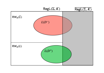
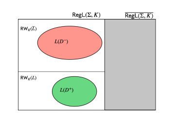
Definition 3.10 (Completeness).
A 3DFA over is complete w.r.t. the timed language if the timed language of , when interpreted as a DERA, is a subset of , i.e., ; and the timed language of , when interpreted as a DERA, is a subset of , i.e., .
Lemma 3.11.
Let be a timed language over recognized by a -DERA over , then for any 3DFA over , is complete w.r.t. iff and .
Proof 3.12.
However, to show the minimality in the number of states of the final DERA returned by our greybox learning algorithm, we introduce strong-completeness, by strengthening the condition on the language accepted by a 3DFA as follows: , and . In other words, we require that all the inconsistent words lead to a “don’t care” state in .
Definition 3.13 (Strong-completeness).
A 3DFA over is strongly-complete w.r.t. the timed language if is complete w.r.t. and additionally, every region word that is strongly accepted or strongly rejected by must be consistent, i.e., if and ; and and .
Corollary 3.14.
Let be a timed language over recognized by a -DERA over , then for any 3DFA over , is strongly-complete w.r.t. iff and . is strongly-complete w.r.t. iff and .
A pictorial representation of completeness and strong-completeness are given in Figure 2. A dual notion of completeness, called soundness can also be defined in this context, however, since we will only need that notion for showing the termination of tLSep, we will introduce it in the next section.
4 The tLSep algorithm
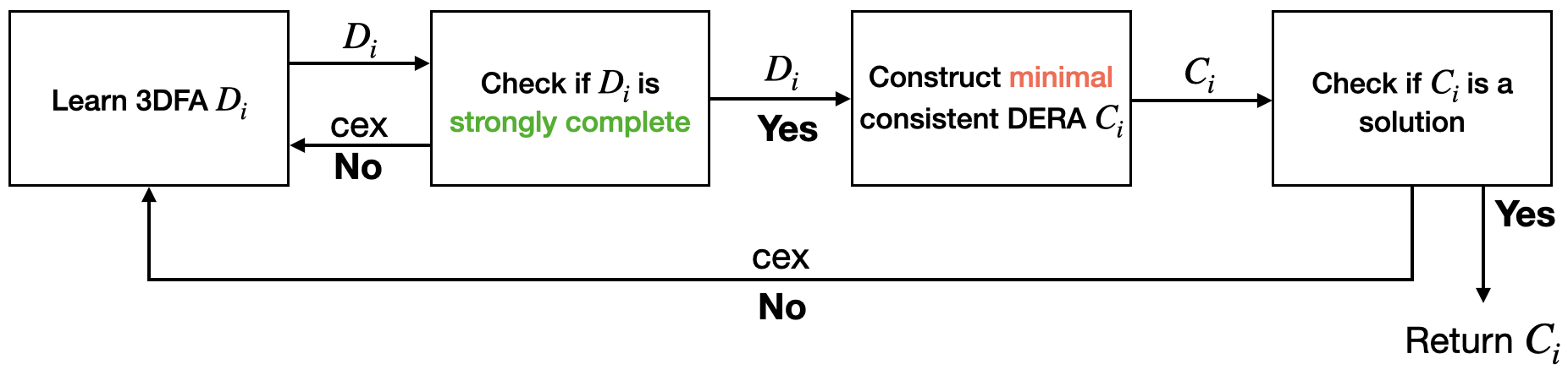
To learn a ERA-recognizable language , we adopt the following greybox learning algorithm, that is an adaptation of the separation algorithm proposed in [7]. The main steps of the algorithm are the following: we first learn a (strongly-)complete 3DFA that maps finite words on the alphabet to , where means “accept”, means “reject”, and means “don’t care”. The 3DFA is used to represent a family of regular languages such that . We then extract from a minimal automaton that is compatible with the 3DFA , i.e., such that . Finally, we check, using two inclusion queries, if satisfies the equation . If this is the case then we return , otherwise, we use the counterexample to this equality check to learn a new 3DFA . We now give details of the greybox in the following subsections, and we conclude this section with the properties of our algorithm.
4.1 Learning the 3DFA
In this step, we learn the 3DFA , by relying on a modified version of . Similar to , we maintain an observation table , where (the set of ‘prefixes’) and (the set of ‘suffixes’) are sets of region words. is a function that maps the region words , where , to if , if and to if . Crucially, we restrict membership queries exclusively to consistent region words. The rationale is that queries for inconsistent words are redundant, given our understanding that such words invariably yield a “” response from the Teacher. This approach streamlines the learning phase by reducing the number of necessary membership queries. We can see the 3DFA defining a space of solutions for the automaton that must be discovered.
4.2 Checking if the 3DFA is (strongly-)complete
We can interpret the 3DFA as the definition for a space of solutions for recognizing the region language . In order to ensure that the final DERA of our algorithm has the minimum number of states, we rely on the fact that at every iteration , the 3DFA is strongly-complete. To this end, we show the following result:
Lemma 4.1.
Let be a timed language, and be a K-DERA with the minimum number of states accepting L. Let be the minimal consistent DFA such that . If is strongly-complete, then .
Proof 4.2.
We shall show that is consistent with . First, if , then (since strongly-complete), therefore from Corollary 3.14, and hence . For the other side, if , then , and again from Corollary 3.14, , which is equivalent to . Now note that , and hence , and so, . Therefore, is consistent with . From hypothesis, is the minimal DFA that is consistent with . Therefore, it follows that .
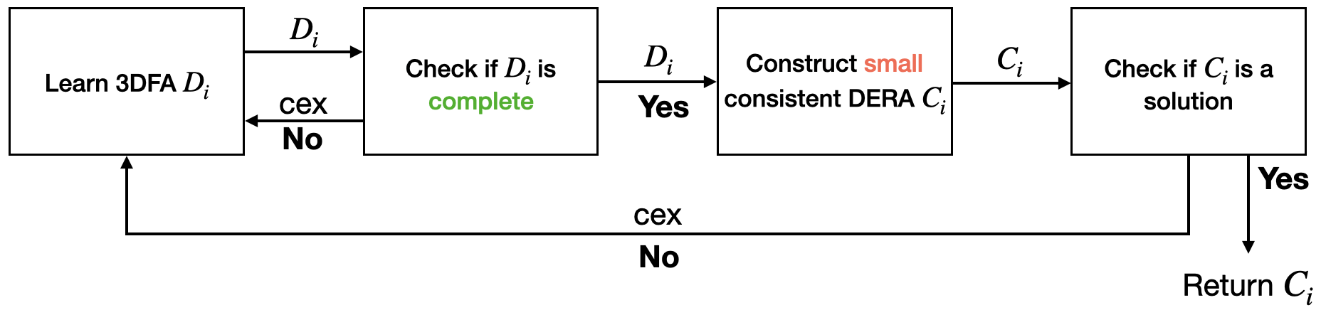
The lemma above implies that if we compute a minimal consistent DFA from a strongly-complete DFA w.r.t. the timed language and if this satisfies Equation 1, then recognizes (when it is interpreted as a DERA) and it has the minimum number of states among every DERA recognizing . The two requirements – being strongly-complete and being a minimal consistent DFA – are necessary to ensure that the resulting DERA for has the minimum number of states. However, checking both of these requirements are computationally expensive. First, for strong-completeness, one needs to check that no inconsistent region word is strongly accepted or strongly rejected by the 3DFA . This can be done by checking if every region word that is either strongly accepted or strongly rejected by is accepted by a DFA recognizing the regular language – this is computationally hard due to the size of the latter. Second, computing a minimal consistent DFA from requires essentially to find a DFA that accepts every region word that is strongly accepted by and rejects every region word that is strongly rejected by . This is a generalization of the problem of finding a DFA with minimum number of states accepting a set of positive words and rejecting a set of negative words, which is known – due to the works of Gold [11] – to be a computationally hard problem. In practice, we generally do not require (as is also remarked in [7]) the automaton with the minimum number of states, instead it is sufficient to compute an automaton with a small number of states – provided it makes the algorithm computationally easier. To this end, instead of implementing the algorithm depicted in Figure 3, we instead implement the algorithm depicted in Figure 4 that employs two relaxations – (i) we only compute a complete DFA , and (ii) we only compute a small (not necessarily minimal) consistent with . Whereas checking whether a DFA is complete or not can be done by checking the two inclusions mentioned in Definition 3.10, we present a heuristic for computing a small consistent DFA in the next section. These two relaxations come at the cost of minimality of the solution, however, we show in Theorem 4.14 that this version of our algorithm still correctly computes a DERA recognizing . As we will see in Section 5, our implementation returns an automaton with a reasonably small, sometimes minimum, number of states.
4.3 Computing a small candidate from
In this section, we detail a heuristic that computes a small candidate DFA from a DFA that is complete with respect to . For the rest of this section, we fix the notation for the DFA .
The first step is to find the set of all pairs of states that are incompatible in . Two states are incompatible if there exists a region word s.t. leads one of them to an accepting state in and another to a rejecting state in . Notice that, in the above definition, one does not take into account the timing constraints of a word, and that is precisely the reason why in the final automaton, the inconsistent words may lead to any state, unlike in a “simple DERA” for the corresponding timed language, where the inconsistent words must be rejected syntactically by the automaton, enabling it to be (possibly) smaller than the “minimal simple DERA”.
We recursively compute the set of incompatible pairs of states as follows: initially add every pair into where , ; then recursively add new pairs as long as possible: add a new pair into s.t. there exists a letter s.t. and and .
The second step is to find the set of all -maximal sets that are compatible in . A set of states of is compatible if it does not contain any incompatible pair. The set of maximal sets of compatible pairs, denoted by , can be computed recursively as follows: initially, ; at any iteration, if there exists a set s.t. there exists a pair , we do the following operation: , with the condition that is added to the set only if there exists no in such that , and similarly for . Then we can prove the correctness of the above procedure in the following manner.
Theorem 4.3.
The above procedure terminates. Moreover, the set returned by the algorithm is the set of all maximal compatible sets in the 3DFA .
Proof 4.4.
Termination: The number of distinct subsets of is bounded by , where denotes the size of . Notice that, at every iteration, a set from is chosen and (at most two) sets with ‘strictly’ smaller size gets added to . Therefore, it is not possible for the same set to be added twice along the procedure. In the worst case, it can contain all the distinct subsets of . Since the number of such sets is bounded and no set is added twice, the procedure terminates.
Correctness: Let us denote by the set , and let denote the sets obtained after each iteration of the algorithm. Let us denote by the set returned by the algorithm, i.e., . The proof of correctness follows from the following lemma:
Lemma 4.5.
All sets in are compatible, and are maximal w.r.t the subset ordering, i.e., they form a -antichain. Furthermore, for every that is compatible, there is some such that .
Proof 4.6.
First, if contains a set which is not compatible, then would be deleted at the -th iteration of the algorithm, which contradicts the fact that . Therefore, all sets in are compatible.
The second statement can be shown by induction on .
Base case: is maximal.
Induction hypothesis: Suppose all sets in is maximal.
Induction step: Suppose we delete the set at iteration , and let be the incompatible pair in . Then iff there is no s.t. iff is maximal (same argument for ). Since these are the only two sets that could possibly be added to , an since by induction hypothesis, all sets in are maximal, the statement follows also for .
The third statement can also be proved by induction on .
Base case: Since , and since , the statement trivially holds.
Induction hypothesis: Suppose the statement holds for .
Induction step: Let be a compatible set. Let be the set selected in iteration with the incompatible pair being . From induction hypothesis, there exists a set such that .
Case 1. . In this case, as well, and hence the result follows.
Case 2. is . Now, note that, in place of , the set contains two sets (both are compatible, due to Lemma 4.5) where and , and is an incompatible pair. Now, since is consistent, (and also, , ) cannot contain both the states . Therefore, if , and if .
In the final step, we define a DFA , where: ; s.t. , and has the highest cardinality; for any , and , define s.t. , and has the largest cardinality; and .
Note that, the DFA constructed from the 3DFA is not unique in the sense that (1) there might be more than one possible in s.t. , and (2) there might be more than one possible in such that . Also, it is important here to note that, one can apply further heuristics at this step, in particular, while adding a new transition from on , if there is already some maximal set that has been discovered previously, set the target of this transition to , even if it is not of maximum cardinality.
Lemma 4.7.
For any 3DFA , the procedure described above is well-defined. Then for any constructed according to the procedure, is consistent with , i.e., and .
Proof 4.8.
Well-definedness: First, notice that, from Lemma 4.5, there must exist a set such that . Second, let be any maximal set in , and . Let . Notice that, since is compatible, therefore has to be a compatible set. Indeed, if there exists a pair of states in that are incompatible, then there must exist in such that and are two transitions in , and hence are also incompatible contradicting the hypothesis that is compatible. Now that we have shown that must be a compatible set, again by Lemma 4.5, there must exist such that . This concludes the proof.
Consistency: Consider any constructed according to the procedure from the 3DFA . Suppose is a region word over (not necessarily consistent). Let be the unique run of in the 3DFA . By applying Lemma 4.5 on the transitions of , in particular by induction, one can show that there exists a unique run , where for all , is a state in s.t. . Now suppose, . Then, . By definition of (the set of accepting states of ), , which implies that . A similar argument can be used to show that for any , . This concludes the proof.
Taking intersection with on both sides, together with Lemma 3.6, we get the following corollary:
Corollary 4.9.
, and .
4.4 Checking if is a solution
Now that has been extracted from , we can query the with two inclusion queries that check if . If the answer is yes, then is a solution to our the learning problem, and we return the automaton ; otherwise, the Teacher returns a counterexample – a consistent region word that is either accepted by but is not in , or a consistent region word that is rejected by but is in . Notice that the equality check has been defined above as an equality check between two timed languages, whereas, the counterexamples returned by the Teacher are region words. This is not contradictory, indeed, one can show a similar result to Lemma 3.8 that iff . More details on how the counter-example is extracted from the answer received from the Teacher is described in Section 5. We will show in Lemma 4.12 that a counterexample to the equality check is also a ‘discrepancy’ in the 3DFA . Therefore, this counterexample is used to update the observation table as in to produce the subsequent hypothesis .
4.5 Correctness of the tLSep algorithm
Definition 4.10 (Soundness).
A 3DFA over is sound w.r.t. the timed language if the timed language of , when interpreted as a DERA, contains , i.e., ; and the timed language of , when interpreted as a DERA, contains , i.e., .
Similar to Lemma 3.11, one can show the following result:
Lemma 4.11.
Let be a timed language over recognized by a -DERA over , then for any 3DFA over , is sound w.r.t. iff and .
The following lemma shows that a counter-example of the equality check in Section 4.4 is also a counter-example to the soundness of :
Lemma 4.12.
If a counter-example is generated for the equality check against , then the corresponding 3DFA is not sound w.r.t. .
Proof 4.13.
Recall from Corollary 4.9 that, , and . Let be a counter-example for the equality check, then:
(1) either there exists a consistent region word , which implies . Hence, is not sound w.r.t .
(2) or, there exists a consistent region word . Since is consistent, using Lemma 3.4, we can deduce that , which implies . Hence, is not sound w.r.t. .
We can prove the following using similar lines of arguments as in [7].
Theorem 4.14.
Let be a timed language over recognizable by a ERA given as input to the tLSep algorithm. Then,
-
1.
the algorithm tLSep terminates,
-
2.
the algorithm tLSep is correct, i.e., letting be the automaton returned by the algorithm, ,
-
3.
at every iteration of tLSep, if strong-completeness is checked for 3DFA , and if a minimization procedure is used to construct , then has a minimal number of states.
Proof 4.15.
1. One can define the following ‘canonical’ 3DFA over from as follows: for every consistent region word s.t. , define ; for every consistent region word s.t. , define ; and for every inconsistent region word , define . It is then easy to verify that is sound and complete w.r.t. . Due to Lemma 4.12, at iteration , a counterexample is produced only if the 3DFA is not sound. Notice also that, from Lemma 3.1 and Lemma 3.6, the languages , , and are regular languages. Therefore, the 3DFAs constructed from the observation table at every iteration of tLSep algorithm, as described in Section 4.1, gradually converges to the canonical sound and complete 3DFA (as shown in the case of regular separability in [12]).
2. Since is the final automaton, it must be the case that when an equality check was asked to the teacher with hypothesis , no counter-example was generated, and hence .
3. This statement follows from Lemma 4.1 together with the fact that is the minimal consistent DFA for .
5 Implementation and its performance
We have made a prototype implementation of tLSep in Python. Parts of our implementation are inspired from the implementation of in AALpy [17]. For the experiments, we assume that the Teacher has access to a DERA recognizing the target timed language . Below, we describe how we implement the sub-procedures. Note that, in our implementation, we check for completeness, and not for strong-completeness, of the 3DFA’s.
Emptiness of region words.
Since we do not perform a membership query for inconsistent region words, before every membership query, we first check if the region word is consistent or not (in agreement with our greybox learning framework described in Page 3.1). The consistency check is performed by encoding the region word as an SMT formula in Linear Real Arithmetic and then checking (using the SMT solver Z3 [9]) if the formula is satisfiable or not. Unsatisfiability of the formula implies the region word is inconsistent.
Inclusion of Timed languages.
We check inclusion between timed languages recognizable by ERA in two situations: (i) while making the 3DFA complete (cf. Definition 3.10), and (ii) during checking if the constructed DERA recognizes (cf. Definition 4.10). Both of these checks can be reduced to checking emptiness of appropriate automata. We perform the emptiness checks using the reachability algorithm (covreach) implemented inside the tool TChecker [13].
Counterexample processing.
When one of the language inclusions during completeness checking returns False, we obtain a ‘concrete’ path from TChecker that acts as a certificate for non-emptiness. The path is of the form:
Since the guards present in the automata are region words, every guard present in the product automaton is also a region word. From we then construct the region word . We then use the algorithm proposed by Rivest-Schapire [14, 18] to compute the ‘witnessing suffix’ from and then add to the set of suffixes () of the observation table. On the other hand, when we receive a counterexample during the soundness check, we add all the prefixes of this counterexample to the set instead. Note that, the guards present on the transitions in our output are simple constraints, and not constraints.
We now compare the performance of our prototype implementation of tLSep against the algorithm proposed by Waga in [24] on a set of synthetic timed languages and on a benchmark taken from their tool LearnTA. We witness encouraging results, among those, we stress on the important ones below.
Minimality.
We have shown in Section 4 that if one ensures strong-completeness of the 3DFAs throughout the procedure, then the minimality in the number of states is assured. However, this is often the case even with only checking completeness. For instance, recall our running example from Figure 1. For this language, our algorithm was able to find a DERA with only two states (depicted in Figure 6(a)) – which is indeed the minimum number of states. On the other hand, LearnTA does not claim minimality in the computed automaton, and indeed for this language, they end up constructing the automaton in Figure 6(b) instead. Note that for the sake of clarity, we draw a single edge from to on in Figure 6(a), however, our implementation constructs several parallel edges (on ) between these two states, one for each constraint in .
Explainability.
From a practical point of view, explainability of the output automaton is a very important property of learning algorithms. One would ideally like the learning algorithm to return a ‘readable’, or easily explainable, model for the target language. We find some of the automata returned by tLSep are relatively easier to understand than the model returned by LearnTA. This is essentially due to the readability of ERA over TA. A comparative example can be found in Figure 5.
Efficiency.
We treat completeness checks for a 3DFA and language-equivalence checks for a DERA, as equivalence queries (EQ). Note that, EQ’s are not new queries, these are merely (at most) two Inclusion Queries (IQ). We report on the number of queries for tLSep and LearnTA in Table 2 on a set of examples. For both the algorithms, we only report on the number of queries ‘with memory’ in the sense that we fetch the answer to a query from the memory if it was already computed. Notice that LearnTA uses two types of membership queries, called symbolic queries (s-MQ) and timed-queries (t-MQ), and in most of the examples, tLSep needs much lesser number of membership queries than LearnTA.
Although the class of ERA-recognizable languages is a strict subclass of DTA-recognizable languages, we found a set of benchmarks from the LearnTA tool, that are in fact event-recording automata (after renaming the clocks). This example is called Unbalanced, Table 2 shows that tLSep uses significantly lesser number of queries than LearnTA for these, illustrating the gains of our greybox approach.
Below, we give brief descriptions of languages that we have learnt using our tLSep algorithm. The timed language (ex1) has untimed language , where in every such four letter block, the second must occur before time unit of the first and the second must occur after time unit since the first . The language (ex2) has untimed language , where the first happens at time unit and every subsequent occurs exactly time unit after the preceding . The timed language (ex3) consists of timed words whose untimed language is , and the first can occur at any time, then there can be several ’s all exactly time unit after , and then the last occurs strictly after time unit since the first . We also consider the language (ex4) represented by the automaton in Figure 5(a) (this language is taken from [12]), for whose language, as we have described, tLSep constructs a relatively more understandable automaton compared to LearnTA.
| Model | tLSep | LearnTA | |||||||
| Figure 1 | 1 | 4 | 2 | 98 | 8 | 5 | 230 | 219 | 4 |
| ex1 | 1 | 5 | 2 | 219 | 11 | 6 | 296 | 365 | 4 |
| ex2 | 1 | 3 | 2 | 220 | 12 | 7 | 247 | 233 | 5 |
| ex3 | 2 | 4 | 2 | 87 | 7 | 4 | 123 | 173 | 3 |
| ex4 | 1 | 3 | 1 | 26 | 5 | 3 | 40 | 43 | 2 |
| Unbalanced-1 | 1 | 5 | 3 | 421 | 17 | 12 | 1717 | 2394 | 6 |
| Unbalanced-2 | 2 | 5 | 3 | 1095 | 27 | 20 | 7347 | 13227 | 10 |
| Unbalanced-3 | 3 | 5 | 3 | 2087 | 37 | 28 | 21200 | 45400 | 17 |
6 Discussions
Our grey box learning algorithm can produce automata with a minimal number of states, equivalent to the minimal DERA for the target language. Currently, the transitions are labeled with region constraints. In the future, we plan to implement a procedure that consolidates edges labeled with the same event and regions, whose unions are convex, into a single edge with a zone constraint. This planned procedure aims to not only maintain an automaton with the fewest possible states, but also to minimize the number of edges and zones. Such optimization could further enhance the readability of the models we produce, thereby improving explainability—an increasingly important aspect of machine learning.
Building on our proposed future work above, we also aim to refine our approach to membership queries. Instead of defaulting to queries on regions where it may not be necessary, we plan to consider queries on zones. If the response from the Teacher is not uniform across the zone, only then will we break down the queries into more specific sub-queries, ending in regions if necessary. This strategy will necessitate revising the current learning protocol we use, but exploring these alternatives could enhance the efficiency and effectiveness of our learning process. Similar ideas have been used in [15].
Throughout this paper, we follow the convention used in prior research [12, 24] that the parameter is predetermined (the maximal constant against which the clocks are compared). Similarly, in our experimental section, we assume we know which events need to be tracked by a clock. While these assumptions are typically reasonable in practice, it is possible to consider a more flexible approach. We could start with no predetermined events to track with clocks and only introduce clocks for events and update the maximum constant, as needed. These could be inferred from the counterexamples provided by the Teacher.
Overall, we believe the greybox learning framework described in this work may also be well-suited for other classes of languages that enjoy a similar condition like Equation 1, where the automaton can be of relatively smaller size, while a canonical model recognizing might be too large.
References
- [1] Andreas Abel and Jan Reineke. Gray-box learning of serial compositions of mealy machines. In NFM, volume 9690 of Lecture Notes in Computer Science, pages 272–287. Springer, 2016.
- [2] Rajeev Alur and David L. Dill. A theory of timed automata. Theor. Comput. Sci., 126(2):183–235, 1994.
- [3] Rajeev Alur, Limor Fix, and Thomas A. Henzinger. Event-clock automata: A determinizable class of timed automata. Theor. Comput. Sci., 211(1-2):253–273, 1999.
- [4] Jie An, Lingtai Wang, Bohua Zhan, Naijun Zhan, and Miaomiao Zhang. Learning real-time automata. Sci. China Inf. Sci., 64(9), 2021.
- [5] Dana Angluin. Learning regular sets from queries and counterexamples. Inf. Comput., 75(2):87–106, 1987.
- [6] Véronique Bruyère, Bharat Garhewal, Guillermo A. Pérez, Gaëtan Staquet, and Frits W. Vaandrager. Active learning of mealy machines with timers. CoRR, abs/2403.02019, 2024. URL: https://doi.org/10.48550/arXiv.2403.02019.
- [7] Yu-Fang Chen, Azadeh Farzan, Edmund M. Clarke, Yih-Kuen Tsay, and Bow-Yaw Wang. Learning minimal separating dfa’s for compositional verification. In TACAS, volume 5505 of Lecture Notes in Computer Science, pages 31–45. Springer, 2009.
- [8] Lénaïg Cornanguer, Christine Largouët, Laurence Rozé, and Alexandre Termier. TAG: learning timed automata from logs. In AAAI, pages 3949–3958. AAAI Press, 2022.
- [9] Leonardo Mendonça de Moura and Nikolaj S. Bjørner. Z3: an efficient SMT solver. In TACAS, volume 4963 of Lecture Notes in Computer Science, pages 337–340. Springer, 2008.
- [10] David L. Dill. Timing assumptions and verification of finite-state concurrent systems. In Automatic Verification Methods for Finite State Systems, volume 407 of Lecture Notes in Computer Science, pages 197–212. Springer, 1989.
- [11] E. Mark Gold. Complexity of automaton identification from given data. Inf. Control., 37(3):302–320, 1978. doi:10.1016/S0019-9958(78)90562-4.
- [12] Olga Grinchtein, Bengt Jonsson, and Martin Leucker. Learning of event-recording automata. Theor. Comput. Sci., 411(47):4029–4054, 2010.
- [13] Frédéric Herbreteau and Gerald Point. Tchecker. URL: https://github.com/ticktac-project/tchecker.
- [14] Malte Isberner and Bernhard Steffen. An abstract framework for counterexample analysis in active automata learning. In ICGI, volume 34 of JMLR Workshop and Conference Proceedings, pages 79–93. JMLR.org, 2014.
- [15] Shang-Wei Lin, Étienne André, Jin Song Dong, Jun Sun, and Yang Liu. An efficient algorithm for learning event-recording automata. In ATVA, volume 6996 of Lecture Notes in Computer Science, pages 463–472. Springer, 2011.
- [16] Mark Moeller, Thomas Wiener, Alaia Solko-Breslin, Caleb Koch, Nate Foster, and Alexandra Silva. Automata learning with an incomplete teacher. In ECOOP, volume 263 of LIPIcs, pages 21:1–21:30. Schloss Dagstuhl - Leibniz-Zentrum für Informatik, 2023.
- [17] Edi Muškardin, Bernhard Aichernig, Ingo Pill, Andrea Pferscher, and Martin Tappler. Aalpy: an active automata learning library. Innovations in Systems and Software Engineering, 18:1–10, 03 2022. doi:10.1007/s11334-022-00449-3.
- [18] Ronald L. Rivest and Robert E. Schapire. Inference of finite automata using homing sequences. Inf. Comput., 103(2):299–347, 1993.
- [19] Martin Tappler, Bernhard K. Aichernig, Kim Guldstrand Larsen, and Florian Lorber. Time to learn - learning timed automata from tests. In FORMATS, volume 11750 of Lecture Notes in Computer Science, pages 216–235. Springer, 2019.
- [20] Yu Teng, Miaomiao Zhang, and Jie An. Learning deterministic multi-clock timed automata. In HSCC, pages 6:1–6:11. ACM, 2024.
- [21] Frits W. Vaandrager. Model learning. Commun. ACM, 60(2):86–95, 2017.
- [22] Frits W. Vaandrager, Roderick Bloem, and Masoud Ebrahimi. Learning mealy machines with one timer. In LATA, volume 12638 of Lecture Notes in Computer Science, pages 157–170. Springer, 2021.
- [23] Sicco Verwer, Mathijs de Weerdt, and Cees Witteveen. One-clock deterministic timed automata are efficiently identifiable in the limit. In LATA, volume 5457 of Lecture Notes in Computer Science, pages 740–751. Springer, 2009.
- [24] Masaki Waga. Active learning of deterministic timed automata with myhill-nerode style characterization. In CAV (1), volume 13964 of Lecture Notes in Computer Science, pages 3–26. Springer, 2023.
- [25] Runqing Xu, Jie An, and Bohua Zhan. Active learning of one-clock timed automata using constraint solving. In ATVA, volume 13505 of Lecture Notes in Computer Science, pages 249–265. Springer, 2022.