Gribov horizon, Polyakov loop and finite temperature

Within $SU(N)$ Yang-Mills gauge theories, it is observed that the asymptotic particle spectrum does not contain the elementary excitations of quarks and gluons. These color charged objects are confined into color neutral bound states: this is the so-called color confinement phenomenon. The best theoretical explanation we have for confinement is due to non-perturbative infrared effects. Different criteria for confinement have been proposed (see the pedagogical introduction [1]). A very natural observation is that gluons should not belong to the physical spectrum in a confining theory. Hence, non-perturbative effects should dress the perturbative propagator in such a way that the positivity conditions are violated. Therefore, it does not belong to the physical spectrum anymore. The Polyakov loop [2] was proposed as an order parameter for the confinement/deconfinement phase transition via its connection to the free energy of a (very heavy) quark. The importance to clarify the interplay between these two different points of view (nonperturbative Green function’s behaviour vs. Polyakov loop) can be understood by observing that while there are, in principle, infinitely many different ways to write down a gluon propagator which violates the positivity conditions, it is very likely that only few of these ways turns out to be compatible with the Polyakov criterion.

One of the most fascinating non-perturbative infrared effects is related to the appearance of Gribov copies [3], that represent an intrinsic overcounting of the gauge-field configurations which the perturbative gauge-fixing procedure is unable to take care of. The presence of Gribov copies induces the existence of non-trivial zero modes of the Faddeev-Popov operator, which make the path integral ill defined. Soon after Gribov’s seminal paper, Singer showed that any true gauge condition, as the Landau gauge¹¹1We shall work exclusively with the Landau gauge here., presents this obstruction [4] (see also [5]).

The most effective method to eliminate Gribov copies, at leading order proposed by Gribov himself, and refined later on by Zwanziger [3, 6, 7, 8], corresponds to restricting the path integral to the first Gribov region, which is the region in the functional space of gauge potentials over which the Faddeev-Popov operator is positive definite. The Faddeev–Popov operator is Hermitian in the Landau gauge, so it makes sense to discuss its sign. In [9, 10] Dell’Antonio and Zwanziger showed that all the orbits of the theory intersect the Gribov region, indicating that no physical information is lost when implementing this restriction. Even though this region still contains copies [11], this restriction has remarkable effects. In fact, due to the presence of a dynamical (Gribov) mass scale, the gluon propagator is suppressed while the ghost propagator is enhanced in the infrared. More general, an approach in which the gluon propagator is “dressed” by non-perturbative corrections which push the gluon out of the physical spectrum leads to propagators and glueball masses in agreement with the lattice data [12, 13].

For all these reasons, it makes sense to compute the vacuum expectation value of the Polyakov loop when we eliminate the Gribov copies using the Gribov–Zwanziger (GZ) approach. Related computations are available using different techniques to cope with nonperturbative propagators at finite temperature, see e.g. [14, 15, 16, 17, 18, 19, 20, 21, 22, 23, 24]. In [25, 26, 27], it was already pointed out that the Gribov–Zwanziger quantization offers an interesting way to illuminate some of the typical infrared problems for finite temperature gauge theories. Therefore, in the present work, we recapitulate the paper [28], and present their main results.

In this Section we give a brief overlook of the Gribov ambiguity. The interested reader can find many excellent and fully detailed reviews about this topic (see, for instance, [29, 30]).

Let us start with the Yang–Mills (YM) action in the Euclidean space²²2We shall work in the Euclidean space through this work, therefore, we will do not distinguish if the Lorentz indices are up or down.,

$$S_{\text{YM}}\ =\frac{1}{4}\int d^{4}xF^{a}_{\mu\nu}F^{a}_{\mu\nu}\;,$$

(1)

which is invariant under local $SU(N)$ gauge transformations

$$A_{\mu}\to A^{\prime}_{\mu}=U^{\dagger}A_{\mu}U+U^{\dagger}\partial_{\mu}U\;,$$

(2)

where $U\in SU(N)$ is a finite group element.

When we compute the propagators using path-integral formulation, or any observable of the theory, we must read off the gauge redundance (2). In order to do that, we introduce the following unity into the path integral

$$1=\int\mathcal{D}\alpha\delta(G(A^{\alpha}))\mbox{Det}\left(\frac{\delta G(A^{\alpha})}{\delta\alpha}\right)\;,$$

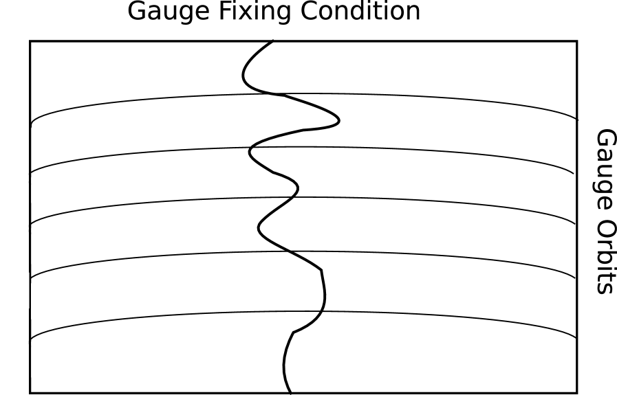
where $G[A]=\partial_{\mu}A^{\mu}$ is the gauge fixing condition (the Landau gauge in this case), while $A^{\alpha}$ is the infinitesimal gauge transformation (2) for $g=\mathds{1}-gt^{a}\alpha^{a}$. The proposal of the gauge fixing condition $G[A]$ is to select one (and only one, if possible) representative of the gauge orbit, see Figure 1. Thus,

$$A^{\alpha}_{\mu}=-D_{\mu}\alpha^{a}\;,$$

(3)

where the covariant derivative is $D_{\mu}^{ab}=(\delta^{ab}\partial_{\mu}-gf^{abc}A_{\mu}^{c})$, $f^{abc}$ being the structure constants of the $SU(N)$ Lie algebra. Using (3), we can write

$$\frac{\delta G(A^{\alpha})}{\delta\alpha}=-\partial^{\mu}D_{\mu}\;,$$

Faddeev and Popov decided to represent the determinant of this quantity as

$$\det\left(-\partial^{\mu}D_{\mu}\right)=\int\mathcal{D}\bar{c}\mathcal{D}c^{b}\exp\left(\bar{c}^{a}\mathcal{M}^{ab}c^{b}\right)\;,$$

where

$$\mathcal{M}^{ab}=-\partial_{\mu}(\partial_{\mu}\delta^{ab}-gf^{abc}A_{\mu}^{c})\;,$$

is the Faddeev–Popov operator. We observe here that $\bar{c},c$ are anticommuting fields, which are scalars under Lorentz transformation, and received the name of Faddeev–Popov ghosts. Now, the Landau gauge fixing condition can be implemented with the help of an auxiliary field $b$, by adding the following term to the action

$$-\int d^{4}xb^{a}\partial^{\mu}A^{a}_{\mu}\;.$$

Therefore, in order to avoid over-counting field configurations, we must compute the path integral of the following Faddeev–Popov action

$$S_{\text{FP}}=S_{\text{YM}}-\int d^{4}x\left(b^{a}\partial^{\mu}A_{\mu}^{a}+\bar{c}^{a}\partial^{\mu}D_{\mu}^{ab}c^{b}\right)\;.$$

(4)

As said before, it is desirable to have only one representative for each gauge orbit. However, this is not possible in the Landau gauge for a non-Abelian Lie algebra, as proven by Gribov [3]. Gribov himself proposed a possible solution to this problem by restricting the domain of integration of the Faddeev-Popov (FP) path-integral, showing at the same time that this leads to a gauge and ghost propagators with a modified infrared behaviour. Moreover, these modified gluon propagators could be interpreted as a signal of confinement, as their poles become complex and do not belong to the Källén-Lehmann spectrum [31].

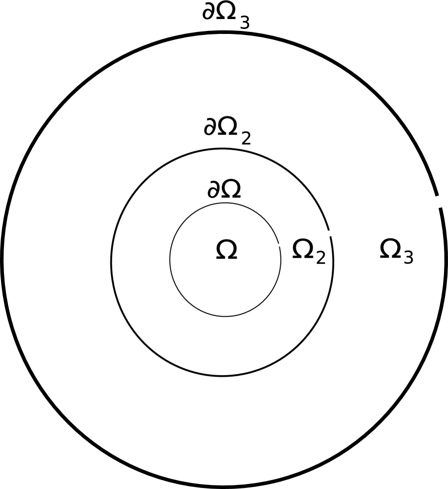
The Gribov region $\Omega$ is the set of all gauge field configurations fulfilling the Landau gauge, $\partial_{\mu}A_{\mu}^{a}=0$ and $\mathcal{M}^{ab}>0$. Namely,

$$\Omega\;=\;\{A_{\mu}^{a}\;;\;\;\partial_{\mu}A_{\mu}^{a}=0\;;\;\;\mathcal{M}^{ab}>0\;\}\;.$$

(5)

As is shown in Figure 2, the space configuration is divided by different horizons $\partial\Omega_{i}$, which are defined by $\mathcal{M}^{ab}=0$.

A great deal of work has been done following the Gribov’s seminal paper, remarkably the construction of a renormalizable action, known as Gribov-Zwanziger (GZ) action [6, 7, 8]. Following these works, the restriction of the domain of integration in the path integral is achieved by adding to the FP action $S_{\text{FP}}$ an additional term $H(A)$, called the horizon term, given by the following non-local expression

$$H(A,\gamma)={g^{2}}\int d^{4}x\;d^{4}y\;f^{abc}A_{\mu}^{b}(x)\left[\mathcal{M}^{-1}(\gamma)\right]^{ad}(x,y)f^{dec}A_{\mu}^{e}(y)\;,$$

(6)

where $\mathcal{M}^{-1}$ stands for the inverse of the FP operator. The partition function can then be written as [3, 6, 7, 8]:

$$Z_{\text{GZ}}\ =\int_{\Omega}\mathcal{D}A\;\mathcal{D}c\;\mathcal{D}\bar{c}\;\mathcal{D}b\;e^{-S_{\text{FP}}}=\int\mathcal{D}A\;\mathcal{D}c\;\mathcal{D}\bar{c}\;\mathcal{D}b\;e^{-(S_{\text{FP}}+\gamma^{4}H(A,\gamma)-V\gamma^{4}4(N^{2}-1))}\;,$$

(7)

where $V$ is the Euclidean space-time volume. The parameter $\gamma$ has the dimension of a mass and is known as the Gribov parameter. We must stress here the fact that this is not a free parameter of the theory. It is a dynamical quantity, being determined in a self-consistent way through a gap equation called the horizon condition [3, 6, 7, 8], given by

$$\left\langle H(A,\gamma)\right\rangle_{\text{GZ}}\ =4V\left(N^{2}-1\right)\;,$$

(8)

where the notation $\left\langle H(A,\gamma)\right\rangle_{\text{GZ}}$ means that the vacuum expectation value of the horizon function $H(A,\gamma)$ has to be evaluated with the measure defined in Eq.(7). An equivalent all-order proof of eq.(8) can be given within the original Gribov no-pole condition framework [3], by looking at the exact ghost propagator in an external gauge field [32].

Although the horizon term $H(A,\gamma)$, eq.(6), is non-local, it can be cast in local form by means of the introduction of a set of auxiliary fields $(\bar{\omega}_{\mu}^{ab},\omega_{\mu}^{ab},\bar{\varphi}_{\mu}^{ab},\varphi_{\mu}^{ab})$, where $(\bar{\varphi}_{\mu}^{ab},\varphi_{\mu}^{ab})$ are a pair of bosonic fields, while $(\bar{\omega}_{\mu}^{ab},\omega_{\mu}^{ab})$ are anti-commuting. The partition function $Z_{\text{GZ}}$ in eq.(7) can be rewritten as [6, 7, 8]

$$Z_{\text{GZ}}\ =\int\mathcal{D}\Phi\;e^{-S_{\text{GZ}}[\Phi]}\;,$$

(9)

where $\Phi$ accounts for the quantizing fields, $A$, $\bar{c}$, $c$, $b$, $\bar{\omega}$, $\omega$, $\bar{\varphi}$, and $\varphi$, while $S_{\text{GZ}}[\Phi]$ is the YM action plus gauge fixing and Gribov–Zwanziger (GZ) terms, in its localized version,

$$S_{\text{GZ}}\ =S_{\text{YM}}\ +S_{\text{gf}}\ +S_{0}+S_{\gamma}\;,$$

(10)

with

$$S_{0}=\int d^{4}x\left({\bar{\varphi}}_{\mu}^{ac}(-\partial_{\nu}D_{\nu}^{ab})\varphi_{\mu}^{bc}-{\bar{\omega}}_{\mu}^{ac}(-\partial_{\nu}D_{\nu}^{ab})\omega_{\mu}^{bc}+gf^{amb}(\partial_{\nu}{\bar{\omega}}_{\mu}^{ac})(D_{\nu}^{mp}c^{p})\varphi_{\mu}^{bc}\right)\;,$$

(11)

and

$$S_{\gamma}=\;\gamma^{2}\int d^{4}x\left(gf^{abc}A_{\mu}^{a}(\varphi_{\mu}^{bc}+{\bar{\varphi}}_{\mu}^{bc})\right)-4\gamma^{4}V(N^{2}-1)\;.$$

(12)

It can be seen from (7) that the horizon condition (8) takes the simpler form

$$\frac{\partial\mathcal{E}_{v}}{\partial\gamma^{2}}=0\;,$$

(13)

which is called the gap equation. The quantity $\mathcal{E}_{v}(\gamma)$ is the vacuum energy defined by

$$e^{-V\mathcal{E}_{v}}=Z_{\text{GZ}}\;\;.$$

(14)

The local action $S_{\text{GZ}}$ in eq.(10) is known as the Gribov–Zwanziger action. Remarkably, it has been shown to be renormalizable to all orders [6, 7, 8, 33, 34, 35, 36, 37]. This important property of the GZ action is a consequence of an extenstive set of Ward identities constraining the quantum corrections in general and possible divergences in particular. In fact, introducing the nilpotent BRST transformations

	$\displaystyle sA_{\mu}^{a}$	$\displaystyle=$	$\displaystyle-D_{\mu}^{ab}c^{b}\;,$
	$\displaystyle sc^{a}$	$\displaystyle=$	$\displaystyle\frac{1}{2}gf^{abc}c^{b}c^{c}\;,$
	$\displaystyle s{\bar{c}}^{a}$	$\displaystyle=$	$\displaystyle b^{a}\;,\qquad\;\;sb^{a}=0\;,$
	$\displaystyle s{\bar{\omega}}_{\mu}^{ab}$	$\displaystyle=$	$\displaystyle{\bar{\varphi}}_{\mu}^{ab}\;,\qquad s{\bar{\varphi}}_{\mu}^{ab}=0\;,$
	$\displaystyle s{\varphi}_{\mu}^{ab}$	$\displaystyle=$	$\displaystyle{\omega}_{\mu}^{ab}\;,\qquad s{\omega}_{\mu}^{ab}=0\;,$		(15)

it can immediately be checked that the GZ action exhibits a soft breaking of the BRST symmetry, as summarized by the equation

$$sS_{\text{GZ}}\ =\gamma^{2}\Delta\;,$$

(16)

where

$$\Delta=\int d^{4}x\left(-gf^{abc}(D_{\mu}^{am}c^{m})(\varphi_{\mu}^{bc}+{\bar{\varphi}}_{\mu}^{bc})+gf^{abc}A_{\mu}^{a}\omega_{\mu}^{bc}\right)\;.$$

(17)

Notice that the breaking term $\Delta$ is of dimension two in the fields. As such, it is a soft breaking and the ultraviolet divergences can be controlled at the quantum level. The properties of the soft breaking of the BRST symmetry of the GZ theory and its relation with confinement have been object of intensive investigation in recent years, see [38, 39, 40, 41, 42, 43, 44, 45, 46, 47]. Here, it suffices to mention that the broken identity (16) is connected with the restriction to the Gribov region $\Omega$. However, a set of BRST invariant composite operators whose correlation functions exhibit the Källén-Lehmann spectral representation with positive spectral densities can be consistently introduced [48]. These correlation functions can be employed to obtain mass estimates on the spectrum of the glueballs [12, 13].

In this Section we shall investigate the confinement/deconfinement phase transition of the $SU(2)$ gauge field theory in the presence of two static sources of (heavy) quarks. The standard way to achieve this goal is by probing the Polyakov loop (PL) order parameter,

$\displaystyle\mathcal{P}=\frac{1}{N}\mbox{Tr}\Braket{Pe^{ig\int_{0}^{\beta}dt\;\;A_{0}(t,x)}}\;,$

(18)

with $P$ denoting path ordering, needed in the non-Abelian case to ensure the gauge invariance of $\mathcal{P}$. In this analytical description of the phase transition involving the PL, one usually imposes the so-called Polyakov gauge on the gauge field, such that, the time-component $A_{0}$ becomes diagonal and independent of (imaginary) time, meaning that the gauge field belongs to the Cartan subalgebra.

In the $SU(2)$ case, if $\frac{1}{2}g\beta\Braket{A_{0}}=\frac{\pi}{2}$ then we are in the “unbroken symmetry phase” (confined or disordered phase), equivalent to $\Braket{{\cal P}}=0$; otherwise, if $\frac{1}{2}g\beta\Braket{A_{0}}<\frac{\pi}{2}$, we are in the “broken symmetry phase” (deconfined or ordered phase), equivalent to $\Braket{{\cal P}}\neq 0$. Since $\mathcal{P}\propto e^{-FT}$ with $T$ the temperature and $F$ the free energy of a heavy quark, it is clear that in the confinement phase, an infinite amount of energy would be required to actually get a free quark. The broken/restored symmetry referred to is the $\mathbb{Z}_{N}$ center symmetry of a pure gauge theory (no dynamical matter in the fundamental representation).

Besides the trivial simplification of the PL, when imposing the Polyakov gauge it turns out that the quantity $\Braket{A_{0}}$ becomes a good alternative choice for the order parameter instead of $\mathcal{P}$. This extra benefit can be proven by means of Jensen’s inequality for convex functions and is carefully explained in [16], see also [15, 17, 18, 19, 20]. As mentioned before, with the Polyakov gauge imposed to the background field $\bar{A}_{\mu}$, the time-component becomes diagonal and time-independent. In other words, we have $\bar{A}_{\mu}(x)=\bar{A}_{0}\delta_{\mu 0}$, with $\bar{A}_{0}$ belonging to the Cartan subalgebra of the gauge group. For instance, in the Cartan subalgebra of $SU(2)$ only the $t^{3}$ generator is present, so that $\bar{A}^{a}_{0}=\delta^{a3}\bar{A}^{3}_{0}\equiv\delta^{a3}\bar{A}_{0}$. As explained in [20], at leading order we then simply find, using the properties of the Pauli matrices,

$$\mathcal{P}=\cos\frac{r}{2}\,,$$

(19)

where we defined

$$r=g\beta\bar{A}_{0}\,,$$

(20)

with $\beta$ the inverse temperature. Just like before, $r=\pi$ corresponds to the confinement phase, while $0\leq r<\pi$ corresponds to deconfinement. With a slight abuse of language, we will refer to the quantity $r$ as the PL hereafter.

In order to probe the phase transition in a quantized non-Abelian gauge field theory, we use the Background Field Gauge (BFG) formalism, detailed in general in e.g. [49]. Within this framework, the effective gauge field will be defined as the sum of a classical field $\bar{A}_{\mu}$ and a quantum field $A_{\mu}$: $a_{\mu}(x)=a_{\mu}^{a}(x)t^{a}=\bar{A}_{\mu}+A_{\mu}$, with $t^{a}$ the infinitesimal generators of the $SU(N)$ symmetry group. The BFG method is a convenient approach, since the tracking of breaking/restoration of the $\mathbb{Z}_{N}$ symmetry becomes easier by choosing the Polyakov gauge for the background field.

Within this framework, it is convenient to define the gauge condition for the quantum field,

$\displaystyle\bar{D}_{\mu}A_{\mu}=0\;,$

(21)

known as the Landau–DeWitt (LDW) gauge fixing condition, where $\bar{D}^{ab}_{\mu}=\delta^{ab}\partial_{\mu}-gf^{abc}\bar{A}^{c}_{\mu}$ is the background covariant derivative. After integrating out the (gauge fixing) auxiliary field $b^{a}$, we end up with the following YM action,

$\displaystyle S_{\text{BFG}}=\int d^{d}x\;\left\{\frac{1}{4}F^{a}_{\mu\nu}F^{a}_{\mu\nu}-\frac{\left(\bar{D}A\right)^{2}}{2\xi}+\bar{c}^{a}\bar{D}_{\mu}^{ab}D^{bd}_{\mu}(a)c^{d}\right\}\;.$

(22)

Notice that, concerning the quantum field $A_{\mu}$, the condition (21) is equivalent to the Landau gauge, yet the action still has background center symmetry. The LDW gauge is actually recovered in the limit $\xi\to 0$, taken at the very end of each computation.

The LDW is also plagued by Gribov ambiguities, and the GZ procedure is applicable also in this instance [28, 50]. Actually dealing with the Gribov copies in the LDW gauge is something very delicate, see [51] and more recently [52]. As we are interested in the qualitative result, we shall take the GZ action modified for the BFG framework (see [53]) as

$$S_{\text{GZ+PLoop}}=\int d^{d}x\;\left\{\frac{1}{4}F^{a}_{\mu\nu}F^{a}_{\mu\nu}-\frac{\left(\bar{D}A\right)^{2}}{2\xi}+\bar{c}^{a}\bar{D}_{\mu}^{ab}D^{bd}_{\mu}(a)c^{d}+\bar{\varphi}_{\mu}^{ac}\bar{D}_{\nu}^{ab}D^{bd}_{\nu}(a)\varphi_{\mu}^{dc}\right.\\ \left.-\bar{\omega}_{\mu}^{ac}\bar{D}_{\nu}^{ab}D^{bd}_{\nu}(a)\omega_{\mu}^{dc}-g\gamma^{2}f^{abc}A_{\mu}^{a}\left(\varphi_{\mu}^{bc}+\bar{\varphi}_{\mu}^{bc}\right)-\gamma^{4}d(N^{2}-1)\right\}\;.$$

(23)

Considering only the quadratic terms of (23), the integration of the partition function gives us the following vacuum energy at one-loop order, defined according to (14),

$$\mathcal{E}_{v}=-\frac{d(N^{2}-1)}{2Ng^{2}}\lambda^{4}+\frac{T}{2V}(d-1)\mbox{Tr}\ln\frac{D^{4}+\lambda^{4}}{\Lambda^{4}}-d\frac{T}{2V}\mbox{Tr}\ln\frac{-D^{2}}{\Lambda^{2}}\;,$$

(24)

where $V$ is the Euclidean space volume, $\lambda^{4}=2Ng^{2}\gamma^{4}$, $\gamma$ is the Gribov parameter, $\overline{D}$ is the covariant background derivative in the adjoint representation defined in (21), and $\Lambda^{2}$ is a scale parameter in order to regularize the result. We stress the fact that in this work we are dealing with $N=2$ colors, although we will frequently continue to explicitly write $N$ dependence for generality of the formulae. Using the usual Matsubara formalism, we have that $D^{2}=(2\pi nT+rsT)^{2}+\vec{q}^{2}$, where $n$ is the Matsubara mode, $\vec{q}$ is the spacelike momentum component, and $s$ is the isospin, given by $-1$, $0$, or $+1$ for the $SU(2)$ case³³3The $SU(3)$ case was handled in [20] as well (see also [54])..

The general trace is of the form

$$I(m^{2},r,s,T)=\frac{1}{\beta V}\mbox{Tr}\ln\frac{-D^{2}+m^{2}}{\Lambda^{2}}=T\sum_{s}\sum_{n=-\infty}^{+\infty}\int\frac{d^{3-\epsilon}q}{(2\pi)^{3-\epsilon}}\ln\left(\frac{(2\pi nT+rsT)^{2}+\vec{q}^{2}+m^{2}}{\Lambda^{2}}\right)\,,$$

(25)

which will be computed numerically.

Let us now investigate what happens to the Gribov parameter $\lambda$ when the temperature is nonzero. Taking the derivative of the effective potential (24) with respect to $\lambda^{2}$ and dividing by $d(N^{2}-1)\lambda^{2}/Ng^{2}$ (as we are not interested in the solution $\lambda^{2}=0$) yields the gap equation for general number of colors $N$:

$$1=\frac{1}{2}\frac{d-1}{d}Ng^{2}\mbox{Tr}\frac{1}{\partial^{4}+\lambda^{4}}+\frac{1}{2}\frac{d-1}{d}\frac{Ng^{2}}{N^{2}-1}\frac{i}{\lambda^{2}}\sum_{s}\left(\frac{\partial I}{\partial m^{2}}(i\lambda^{2},r,s,T)-\frac{\partial I}{\partial m^{2}}(-i\lambda^{2},r,s,T)\right)\;,$$

(26)

where the notation $\partial I/\partial m^{2}$ denotes the derivative of $I$ with respect to its first argument. If we now define $\lambda_{0}$ to be the solution to the gap equation at $T=0$:

$$1=\frac{1}{2}\frac{d-1}{d}Ng^{2}\mbox{Tr}\frac{1}{\partial^{4}+\lambda_{0}^{4}}\;,$$

(27)

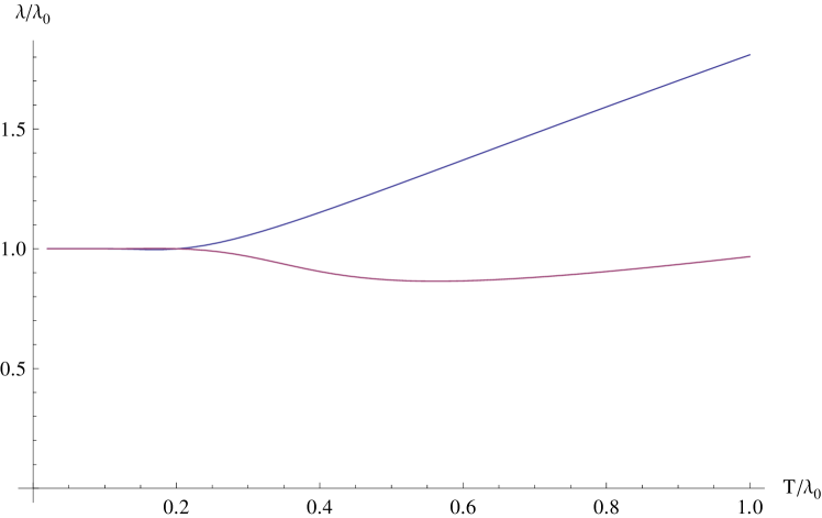
then we can subtract this equation from the general gap equation (26). After dividing through $(d-1)Ng^{2}/2d$ and setting $d=4$ and $N=2$, the result is

$$\int\frac{d^{4}q}{(2\pi)^{4}}\left(\frac{1}{q^{4}+\lambda^{4}}-\frac{1}{q^{4}+\lambda_{0}^{4}}\right)+\frac{i}{3\lambda^{2}}\sum_{s}\left(\frac{\partial I}{\partial m^{2}}(i\lambda^{2},r,s,T)-\frac{\partial I}{\partial m^{2}}(-i\lambda^{2},r,s,T)\right)=0\;,$$

(28)

where now all integrations are convergent. This equation can be easily solved numerically to yield $\lambda$ as a function of temperature $T$ and background $r$, in units $\lambda_{0}$. This is shown in Figure 3.

Let us now investigate the temperature dependence of $r$. We porpose that the physical value of the background field $r$ is found by minimizing the vacuum energy:

$\displaystyle\frac{d}{dr}{\cal E}_{v}=0\;.$

(29)

From the vacuum energy (24) we have

$\displaystyle\frac{\partial\mathcal{E}_{v}}{\partial r}=(d-1)\left[\frac{\partial I}{\partial r}(i\gamma^{2},r,T)+\frac{\partial I}{\partial r}(-i\gamma^{2},r,T)-\frac{d}{(d-1)}\frac{\partial I}{\partial r}(0,r,T)\right]=0\;.$

(30)

The expression (30) was obtained after summation over the possible values of $s$. Furthermore, we used the fact that $I(m^{2},r,+1,T)=I(m^{2},r,-1,T)$ and that $s=0$ accounts for terms independent of $r$, which are cancelled by the derivation w.r.t. $r$. One can get, whenever $s=\pm 1$:

$\displaystyle\frac{\partial I(m^{2},r,T)}{\partial r}=T\int\frac{d^{3}q}{(2\pi)^{3}}\frac{2e^{-\frac{\sqrt{\vec{q}^{2}+m^{2}}}{T}}\sin r}{\left(1+e^{-2\frac{\sqrt{\vec{q}^{2}+m^{2}}}{T}}-2e^{-\frac{\sqrt{\vec{q}^{2}+m^{2}}}{T}}\cos r\right)}\;.$

(31)

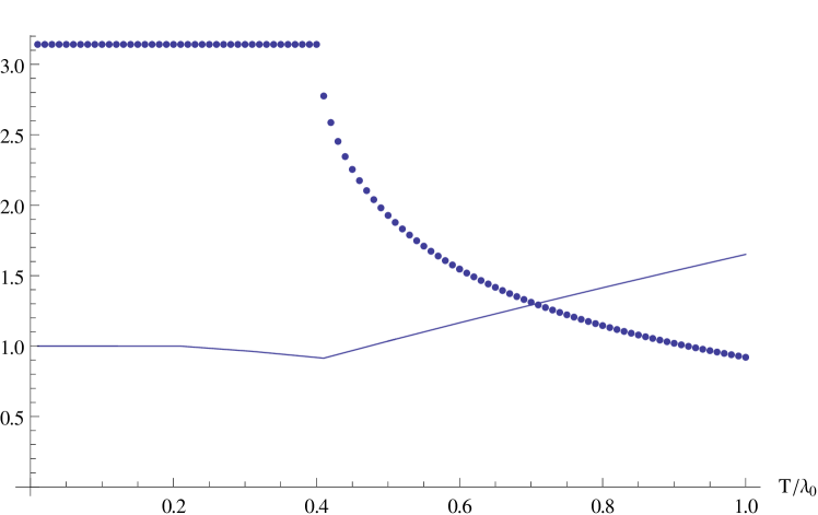
Since (30) is finite, we can numerically obtain $r$ as a function of temperature. From the dotted curve in Figure 4 one can easily see that, for $T>T_{\text{crit}}\approx 0.40\lambda_{0}$, we have $r\neq\pi$, pointing to a deconfined phase, confirming the computations of the previous section. In the same figure, $\lambda(T)$ is plotted in a continuous line. We observe very clearly that the Gribov mass $\lambda(T)$ develops a cusp-like behaviour exactly at the critical temperature $T=T_{\text{crit}}$.

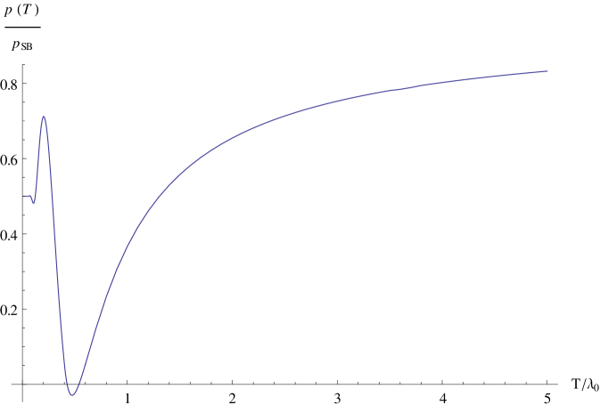
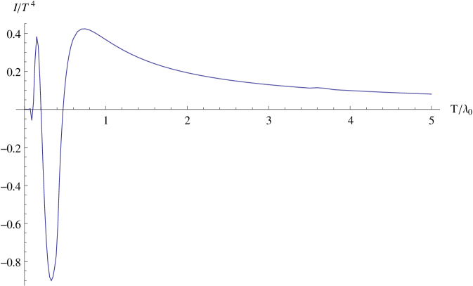
Following [55], we can also extract an estimate for the (density) pressure $p$ and the interaction measure $I/T^{4}$, shown in Figure 5 (left and right respectively). As usual the (density) pressure is defined as

$\displaystyle p=\frac{1}{\beta V}\ln Z_{GZ}\;,$

(32)

which is related to the free energy by $p=-\mathcal{E}_{v}$. Here the plot of the pressure is given relative to the Stefan–Boltzmann limit pressure: $p_{SB}=\kappa T^{4}$, where $\kappa=(N^{2}-1)\pi T^{4}/45$ is the Stefan–Boltzmann constant accounting for all degrees of freedom of the system at high temperature. We subtract the zero-temperature value, such that the pressure becomes zero at zero temperature: $p(T)=-[\mathcal{E}_{v}(T)-\mathcal{E}_{v}(T=0)]$. Namely, after using the $\overline{\mbox{MS}}$ renormalization prescription and choosing the renormalization parameter $\bar{\mu}$ so that the zero temperature gap equation is satisfied,

$\displaystyle{\bar{\mu}}^{2}=\lambda^{2}_{0}e^{-\left(\frac{5}{6}-\frac{32\pi^{2}}{3g^{2}}\right)}\;,$

(33)

we have the following expression for the pressure (in units of $\lambda_{0}^{4}$),

	$\displaystyle-\frac{p(T)}{\lambda_{0}^{4}}$	$\displaystyle=$	$\displaystyle 3\left[I(i\lambda^{\prime 2},r,T^{\prime})+I(-i\lambda^{\prime 2},r,T^{\prime})-\frac{4}{3}I(0,r,T^{\prime})\right]$		(34)
		$\displaystyle+$	$\displaystyle\frac{3}{2}\left[I(i\lambda^{\prime 2},0,T^{\prime})+I(-i\lambda^{\prime 2},0,T^{\prime})-\frac{4}{3}I(0,0,T^{\prime})\right]$
		$\displaystyle-$	$\displaystyle\frac{9\lambda^{\prime 4}}{32\pi^{2}}\left(\ln\lambda^{\prime 2}-\frac{1}{2}\right)-\frac{9}{64\pi^{2}}\;.$

In (34) prime quantities stand for quantities in units of $\lambda_{0}$, while $\lambda$ and $\lambda_{0}$ satisfy their gap equation. The last term of (34) accounts for the zero temperature subtraction, so that $p(0)=0$. Note that the coupling constant does not explicitly appear in (34) and that $\lambda_{0}$ stands for the Gribov parameter at $T=0$.

The interaction measure $I$ is defined as the trace anomaly in units of $T^{4}$, and $I$ is exactly the trace of the stress-energy tensor, given by

$\displaystyle\theta_{\mu\nu}=(p+\epsilon)u_{\mu}u_{\nu}-p\eta_{\mu\nu}\;,$

(35)

with $\epsilon$ being the internal energy density, which is defined as $\epsilon={\cal E}_{v}+Ts$ (with $s$ the entropy density), $u=(1,0,0,0)$ and $\eta_{\mu\nu}$ the (Euclidean) metric of the space-time. Given the thermodynamic definitions of each quantity (energy, pressure and entropy), we obtain

$\displaystyle I=\theta_{\mu\mu}=T^{5}\frac{\partial}{\partial T}\left(\frac{p}{T^{4}}\right)\;.$

(36)

Both quantities display a behavior similar to that presented in [27] (but note that they plot the temperature in units of the critical temperature ($T_{c}$ in their notation), while we use units $\lambda_{0}$). Besides this, and the fact that we included the effect of PL on the Gribov parameter, in [27] a lattice-inspired effective coupling was introduced at finite temperature while we used the exact one-loop perturbative expression, which is consistent with the order of all the computations made here.

However, we notice that at temperatures relatively close to our $T_{c}$, the pressure becomes negative. This is clearly an unphysical feature, possibly related to some missing essential physics. For higher temperatures, the situation is fine and the pressure moreover displays a behaviour similar to what is seen in lattice simulations for the nonperturbative pressure (see [56] for the $SU(3)$ case). A similar problem is present in one of the plots presented in [27, Fig. 4], although no comment is made about it. Another strange feature is the oscillating behaviour of both pressure and interaction measure at low temperatures. Something similar was already observed in [57] where a quark model was employed with complex conjugate quark mass. It is well-known that the gluon propagator develops two complex conjugate masses in GZ quantization, see e.g. [12, 13, 48, 58] for some more details, so we confirm the findings of [57] that, at least at leading order, the thermodynamic quantities develop an oscillatory behaviour. We expect this oscillatory behaviour would in principle also be present in [27] if the pressure and interaction energy were to be computed at lower temperatures than shown there. In any case, the presence of complex masses and their consequences gives us a warning that a certain care is needed when using GZ dynamics, also at the level of spectral properties as done in [59, 60], see also [38, 61].

We have presented here one possible scenario for the confined-deconfined phase transition for a toy model theory, with an internal non-Abelian $SU(2)$ group, where Gribov copies arise. By implementing the PL to the resulting GZ action, gives us a deconfinement critical temperature of $T_{C}\approx 0.40\lambda_{0}$.

In the original paper [28], it is also investigated how this result is modified if we take into account the condensate of the extra fields, an approach known as refined GZ (RGZ). The corrected critical temperature in RGZ scenario is $T_{C}=0.250$ $GeV$, which is not far from the lattice value for $SU(2)$ $T_{C}=0,295$ $GeV$ [62]. However, we must stress here that we pursuit the quality of the transition behaviour rather than quantify the results, as also the lattice values are getting better tuned as the computation machine capabilities are improved.

The thermodynamic pressure has a negative sector. This is an issue that does not only appear in GZ or RGZ, but it is also shared by many different confinement scenarios, see for instance [21]. Actually, the strange behaviour of the thermodynamic variables is related to the complex poles of the GZ propagator, as is explicitly shown in [63]. For that reason, also quark propagators coming from lattice fitting, which are characterized by complex poles, acquire the same pathological thermodynamic behaviour [57, 63]. We expect that a more detailed exploration about the trace anomaly both from thermodynamic and hydrodynamic point of view, could shed some light on this issue.

P. P. acknowledges the warm hospitality of the Centro de Estudios Científicos (CECs) in Valdivia, Chile, during different stages of this work. The Centro de Estudios Científicos (CECs) is funded by the Chilean Government through the Centers of Excellence Base Financing Program of Conicyt.

References

- [1] J. Greensite, An introduction to the confinement problem, Lect. Notes Phys. 821 (2011) 1.
- [2] A. M. Polyakov, Thermal Properties of Gauge Fields and Quark Liberation, Phys. Lett. 72B (1978) 477.
- [3] V. N. Gribov, Quantization of Nonabelian Gauge Theories, Nucl. Phys. B139 (1978) 1.
- [4] I. M. Singer, Some Remarks on the Gribov Ambiguity, Commun. Math. Phys. 60 (1978) 7.
- [5] R. Jackiw, I. Muzinich and C. Rebbi, Coulomb Gauge Description of Large Yang-Mills Fields, Phys. Rev. D17 (1978) 1576.
- [6] D. Zwanziger, Action From the Gribov Horizon, Nucl. Phys. B321 (1989) 591.
- [7] D. Zwanziger, Local and Renormalizable Action From the Gribov Horizon, Nucl. Phys. B323 (1989) 513.
- [8] D. Zwanziger, Renormalizability of the critical limit of lattice gauge theory by BRS invariance, Nucl. Phys. Proc. Suppl. 30 (1993) 221.
- [9] G. Dell’Antonio and D. Zwanziger, Ellipsoidal Bound on the Gribov Horizon Contradicts the Perturbative Renormalization Group, Nucl. Phys. B326 (1989) 333.
- [10] G. Dell’Antonio and D. Zwanziger, Every gauge orbit passes inside the Gribov horizon, Commun. Math. Phys. 138 (1991) 291.
- [11] P. van Baal, More (thoughts on) Gribov copies, Nucl. Phys. B369 (1992) 259.
- [12] D. Dudal, M. S. Guimaraes and S. P. Sorella, Glueball masses from an infrared moment problem and nonperturbative Landau gauge, Phys. Rev. Lett. 106 (2011) 062003 [1010.3638].
- [13] D. Dudal, M. S. Guimaraes and S. P. Sorella, Pade approximation and glueball mass estimates in and with colors, Phys. Lett. B732 (2014) 247 [1310.2016].
- [14] A. Maas, Describing gauge bosons at zero and finite temperature, Phys. Rept. 524 (2013) 203 [1106.3942].
- [15] J. Braun, H. Gies and J. M. Pawlowski, Quark Confinement from Color Confinement, Phys. Lett. B684 (2010) 262 [0708.2413].
- [16] F. Marhauser and J. M. Pawlowski, Confinement in Polyakov Gauge, 0812.1144.
- [17] H. Reinhardt and J. Heffner, The effective potential of the confinement order parameter in the Hamilton approach, Phys. Lett. B718 (2012) 672 [1210.1742].
- [18] H. Reinhardt and J. Heffner, Effective potential of the confinement order parameter in the Hamiltonian approach, Phys. Rev. D88 (2013) 045024 [1304.2980].
- [19] J. Heffner and H. Reinhardt, Finite-temperature Yang-Mills theory in the Hamiltonian approach in Coulomb gauge from a compactified spatial dimension, Phys. Rev. D91 (2015) 085022 [1501.05858].
- [20] U. Reinosa, J. Serreau, M. Tissier and N. Wschebor, Deconfinement transition in SU() theories from perturbation theory, Phys. Lett. B742 (2015) 61 [1407.6469].
- [21] U. Reinosa, J. Serreau, M. Tissier and N. Wschebor, Deconfinement transition in SU(2) Yang-Mills theory: A two-loop study, Phys. Rev. D91 (2015) 045035 [1412.5672].
- [22] C. S. Fischer and J. A. Mueller, Chiral and deconfinement transition from Dyson-Schwinger equations, Phys. Rev. D80 (2009) 074029 [0908.0007].
- [23] T. K. Herbst, M. Mitter, J. M. Pawlowski, B.-J. Schaefer and R. Stiele, Thermodynamics of QCD at vanishing density, Phys. Lett. B731 (2014) 248 [1308.3621].
- [24] A. Bender, D. Blaschke, Y. Kalinovsky and C. D. Roberts, Continuum study of deconfinement at finite temperature, Phys. Rev. Lett. 77 (1996) 3724 [nucl-th/9606006].
- [25] D. Zwanziger, Equation of State of Gluon Plasma from Local Action, Phys. Rev. D76 (2007) 125014 [hep-ph/0610021].
- [26] K. Lichtenegger and D. Zwanziger, Nonperturbative contributions to the QCD pressure, Phys. Rev. D78 (2008) 034038 [0805.3804].
- [27] K. Fukushima and N. Su, Stabilizing perturbative Yang-Mills thermodynamics with Gribov quantization, Phys. Rev. D88 (2013) 076008 [1304.8004].
- [28] F. E. Canfora, D. Dudal, I. F. Justo, P. Pais, L. Rosa and D. Vercauteren, Effect of the Gribov horizon on the Polyakov loop and vice versa, Eur. Phys. J. C75 (2015) 326 [1505.02287].
- [29] R. F. Sobreiro and S. P. Sorella, Introduction to the Gribov ambiguities in Euclidean Yang-Mills theories, in 13th Jorge Andre Swieca Summer School on Particle and Fields Campos do Jordao, Brazil, January 9-22, 2005, 2005, hep-th/0504095.
- [30] N. Vandersickel and D. Zwanziger, The Gribov problem and QCD dynamics, Phys. Rept. 520 (2012) 175 [1202.1491].
- [31] M. Peskin and D. Schroeder, An Introduction to Quantum Field Theory, Advanced book classics. Addison-Wesley Publishing Company, 1995.
- [32] M. A. L. Capri, D. Dudal, M. S. Guimaraes, L. F. Palhares and S. P. Sorella, An all-order proof of the equivalence between Gribov’s no-pole and Zwanziger’s horizon conditions, Phys. Lett. B719 (2013) 448 [1212.2419].
- [33] N. Maggiore and M. Schaden, Landau gauge within the Gribov horizon, Phys. Rev. D50 (1994) 6616 [hep-th/9310111].
- [34] D. Dudal, S. P. Sorella, N. Vandersickel and H. Verschelde, New features of the gluon and ghost propagator in the infrared region from the Gribov-Zwanziger approach, Phys. Rev. D77 (2008) 071501 [0711.4496].
- [35] D. Dudal, J. A. Gracey, S. P. Sorella, N. Vandersickel and H. Verschelde, A Refinement of the Gribov-Zwanziger approach in the Landau gauge: Infrared propagators in harmony with the lattice results, Phys. Rev. D78 (2008) 065047 [0806.4348].
- [36] D. Dudal, S. P. Sorella and N. Vandersickel, More on the renormalization of the horizon function of the Gribov-Zwanziger action and the Kugo-Ojima Green function(s), Eur. Phys. J. C68 (2010) 283 [1001.3103].
- [37] D. Dudal, S. P. Sorella and N. Vandersickel, The dynamical origin of the refinement of the Gribov-Zwanziger theory, Phys. Rev. D84 (2011) 065039 [1105.3371].
- [38] L. Baulieu and S. P. Sorella, Soft breaking of BRST invariance for introducing non-perturbative infrared effects in a local and renormalizable way, Phys. Lett. B671 (2009) 481 [0808.1356].
- [39] D. Dudal, S. P. Sorella, N. Vandersickel and H. Verschelde, Gribov no-pole condition, Zwanziger horizon function, Kugo-Ojima confinement criterion, boundary conditions, BRST breaking and all that, Phys. Rev. D79 (2009) 121701 [0904.0641].
- [40] S. P. Sorella, Gribov horizon and BRST symmetry: A Few remarks, Phys. Rev. D80 (2009) 025013 [0905.1010].
- [41] S. P. Sorella, Gluon confinement, i-particles and BRST soft breaking, J. Phys. A44 (2011) 135403 [1006.4500].
- [42] M. A. L. Capri, A. J. Gomez, M. S. Guimaraes, V. E. R. Lemes, S. P. Sorella and D. G. Tedesco, A remark on the BRST symmetry in the Gribov-Zwanziger theory, Phys. Rev. D82 (2010) 105019 [1009.4135].
- [43] D. Dudal and S. P. Sorella, The Gribov horizon and spontaneous BRST symmetry breaking, Phys. Rev. D86 (2012) 045005 [1205.3934].
- [44] A. Reshetnyak, On Gauge Independence for Gauge Models with Soft Breaking of BRST Symmetry, Int. J. Mod. Phys. A29 (2014) 1450184 [1312.2092].
- [45] A. Cucchieri, D. Dudal, T. Mendes and N. Vandersickel, BRST-Symmetry Breaking and Bose-Ghost Propagator in Lattice Minimal Landau Gauge, Phys. Rev. D90 (2014) 051501 [1405.1547].
- [46] M. A. L. Capri, M. S. Guimaraes, I. F. Justo, L. F. Palhares and S. P. Sorella, Properties of the Faddeev-Popov operator in the Landau gauge, matter confinement and soft BRST breaking, Phys. Rev. D90 (2014) 085010 [1408.3597].
- [47] M. Schaden and D. Zwanziger, Living with spontaneously broken BRST symmetry. I. Physical states and cohomology, Phys. Rev. D92 (2015) 025001 [1412.4823].
- [48] L. Baulieu, D. Dudal, M. S. Guimaraes, M. Q. Huber, S. P. Sorella, N. Vandersickel et al., Gribov horizon and i-particles: About a toy model and the construction of physical operators, Phys. Rev. D82 (2010) 025021 [0912.5153].
- [49] S. Weinberg, The quantum theory of fields. Vol. 2: Modern applications. Cambridge University Press, 2013.
- [50] F. Canfora, D. Hidalgo and P. Pais, The Gribov problem in presence of background field for Yang–Mills theory, Phys. Lett. B763 (2016) 94 [1610.08067].
- [51] D. Dudal and D. Vercauteren, Gauge copies in the Landau–DeWitt gauge: A background invariant restriction, Phys. Lett. B779 (2018) 275 [1711.10142].
- [52] D. Kroff and U. Reinosa, Gribov-Zwanziger type model action invariant under background gauge transformations, Phys. Rev. D98 (2018) 034029 [1803.10188].
- [53] D. Zwanziger, Nonperturbative Modification of the Faddeev-popov Formula and Banishment of the Naive Vacuum, Nucl. Phys. B209 (1982) 336.
- [54] J. Serreau, A perturbative description of the deconfinement transition in Yang-Mills theories, PoS CPOD2014 (2015) 036 [1504.00038].
- [55] O. Philipsen, The QCD equation of state from the lattice, Prog. Part. Nucl. Phys. 70 (2013) 55 [1207.5999].
- [56] S. Borsanyi, G. Endrodi, Z. Fodor, S. D. Katz and K. K. Szabo, Precision SU(3) lattice thermodynamics for a large temperature range, JHEP 07 (2012) 056 [1204.6184].
- [57] S. Benic, D. Blaschke and M. Buballa, Thermodynamic Instabilities in Dynamical Quark Models with Complex Conjugate Mass Poles, Phys. Rev. D86 (2012) 074002 [1206.6582].
- [58] A. Cucchieri, D. Dudal, T. Mendes and N. Vandersickel, Modeling the Gluon Propagator in Landau Gauge: Lattice Estimates of Pole Masses and Dimension-Two Condensates, Phys. Rev. D85 (2012) 094513 [1111.2327].
- [59] N. Su and K. Tywoniuk, Massless Mode and Positivity Violation in Hot QCD, Phys. Rev. Lett. 114 (2015) 161601 [1409.3203].
- [60] W. Florkowski, R. Ryblewski, N. Su and K. Tywoniuk, Bulk viscosity in a plasma of Gribov-Zwanziger gluons, Acta Phys. Polon. B47 (2016) 1833 [1504.03176].
- [61] D. Dudal and M. S. Guimaraes, On the computation of the spectral density of two-point functions: complex masses, cut rules and beyond, Phys. Rev. D83 (2011) 045013 [1012.1440].
- [62] A. Cucchieri, A. Maas and T. Mendes, Infrared properties of propagators in Landau-gauge pure Yang-Mills theory at finite temperature, Phys. Rev. D75 (2007) 076003 [hep-lat/0702022].
- [63] F. Canfora, A. Giacomini, P. Pais, L. Rosa and A. Zerwekh, Comments on the compatibility of thermodynamic equilibrium conditions with lattice propagators, Eur. Phys. J. C76 (2016) 443 [1606.02271].