GROOT: Effective Design of Biological Sequences
with Limited Experimental Data
Abstract.
Latent space optimization (LSO) is a powerful method for designing discrete, high-dimensional biological sequences that maximize expensive black-box functions, such as wet lab experiments. This is accomplished by learning a latent space from available data and using a surrogate model to guide optimization algorithms toward optimal outputs. However, existing methods struggle when labeled data is limited, as training with few labeled data points can lead to subpar outputs, offering no advantage over the training data itself. We address this challenge by introducing GROOT , a GRaph-based Latent SmOOThing for Biological Sequence Optimization. In particular, GROOT generates pseudo-labels for neighbors sampled around the training latent embeddings. These pseudo-labels are then refined and smoothed by Label Propagation. Additionally, we theoretically and empirically justify our approach, demonstrate GROOT’s ability to extrapolate to regions beyond the training set while maintaining reliability within an upper bound of their expected distances from the training regions. We evaluate GROOT on various biological sequence design tasks, including protein optimization (GFP and AAV) and three tasks with exact oracles from Design-Bench. The results demonstrate that GROOT equalizes and surpasses existing methods without requiring access to black-box oracles or vast amounts of labeled data, highlighting its practicality and effectiveness. We release our code at https://anonymous.4open.science/r/GROOT-D554.
1. Introduction
Proteins are crucial biomolecules that play diverse and essential roles in every living organism. Enhancing protein functions or cellular fitness is vital for industrial, research, and therapeutic applications (Huang et al., 2016; Wang et al., 2021). One powerful approach to achieve this is directed evolution, which involves iteratively performing random mutations and screening for proteins with desired phenotypes (Arnold, 1996). However, the vast space of possible proteins makes exhaustive searches impractical in nature, the laboratory, or computationally. Consequently, recent machine learning (ML) methods have been developed to improve the sample efficiency of this evolutionary search (Jain et al., 2022; Ren et al., 2022; Lee et al., 2024). When experimental data is available, these approaches use a surrogate model , trained to guide optimization algorithms toward optimal outputs.
While these methods have achieved state-of-the-art results on various benchmarks, most neglect the scenario of extremely limited labeled data and fail to utilize the abundant unlabeled data. This is a significant issue because exploring protein function and characteristics through iterative mutation in wet-lab is costly (Fowler and Fields, 2014). As later shown in Section 4.2, previous works perform poorly in this context, proving that training with few labeled data points can lead to subpar designs, offering no advantage over the training data itself. One potential solution for dealing with noisy and limited data is to regularize the fitness landscape model, smoothing the sequence representation and facilitating the use of gradient-based optimization algorithms. Although some works have addressed this problem (Section 2), none can optimize effectively in the case of labeled scarcity.
1.1. Contribution
Our work builds on the observation by Trabucco et al. (2022) that surrogate models trained on limited labeled data are vulnerable to noisy labels. This sensitivity can lead the model to sample false negatives or become trapped in suboptimal solutions (local minima) when used for guiding offline optimization algorithms. To address this issue, the ultimate objective is to enhance the predictive ability of , reducing the risk of finding suboptimal solutions. To fulfill this, we propose GROOT , a novel framework designed to tackle the problem of labeled scarcity by generating synthetic sample representations from existing data. From the features encoded by the encoder, we formulate sequences as a graph with fitness values as node attributes and apply Label Propagation (Zhou et al., 2003) to generate labels for newly created nodes synthesized through interpolation within existing nodes. The smoothed data is then fitted with a neural network for optimization. Figure 1 provides an overview of our framework. We evaluate our method on two fitness optimization tasks: Green Fluorescent Proteins (GFP) (Sarkisyan et al., 2016) and Adeno-Associated Virus (AAV) (Bryant et al., 2021). Our results show that GROOT outperforms previous state-of-the-art baselines across all difficulties of both tasks. We also demonstrate that our method performs stably in extreme cases where there are fewer than 100 labeled training sequences, unlike other approaches. Our contributions are summarized as follows:
-
•
We introduce GROOT , a novel framework that uses graph-based smoothing to train a smoothed fitness model, which is then used in the optimization process.
-
•
We theoretically show that our smoothing technique can expand into extrapolation regions while keeping a reasonable distance from the training data. This helps to reduce errors occurring when the surrogate model makes predictions for unseen points too far from the training set.
-
•
We empirically show that GROOT achieves state-of-the-art results across all difficulties in two protein design benchmarks, AAV and GFP. Notably, in extreme cases with very limited labeled data, our approach performs stably, achieving fold fitness improvement in GFP and times higher in AAV compared to the training set.
-
•
We further evaluate GROOT on diverse tasks of different domains (e.g., robotics, DNA) within the Design-Bench. Our experimental results are competitive with state-of-the-art approaches, highlighting the method’s domain-agnostic capabilities.
2. Related work
LSO for Sequence Design
Directed evolution is a traditional paradigm in protein sequence design that has achieved notable successes (Arnold, 2018). Within this framework, various machine learning algorithms have been proposed to improve the sample efficiency of evolutionary searches (Ren et al., 2022; Qiu and Wei, 2022; Emami et al., 2023; Tran and Hy, 2024). However, most of these methods optimize protein sequences directly in the sequence space, dealing with discrete, high-dimensional decision variables. Alternatively, Gómez-Bombarelli et al. (2018) and Castro et al. (2022) employed a VAE model and applied gradient ascent to optimize the latent representation, which is then decoded into biological sequences. Similarly, Lee et al. (2023) used an off-policy reinforcement learning method to facilitate updates in the representation space. Another notable approach (Stanton et al., 2022) involves training a denoising autoencoder with a discriminative multi-task Gaussian process head, enabling gradient-based optimization of multi-objective acquisition functions in the latent space of the autoencoder. Recently, latent diffusion has been introduced for designing novel proteins, leveraging the capabilities of a protein language model (Chen et al., 2023).
Protein Fitness Regularization
The NK model was an early effort to represent protein fitness smoothness using a statistical model of epistasis (Kauffman and Weinberger, 1989). Gómez-Bombarelli et al. (2018) approached this by mapping sequences to a regularized latent fitness landscape, incorporating an auxiliary network to predict fitness from the latent space. Castro et al. (2022) further enhanced this work by introducing negative sampling and interpolation-based regularization into the regularization of latent representation. Additionally, Frey et al. (2024) proposed to learn a smoothed energy function, allowing sequences to be sampled from the smoothed data manifold using Markov Chain Monte Carlo (MCMC). Currently, GGS (Kirjner et al., 2024) is most related to our work by utilizing discrete regularization using graph-based smoothing techniques. However, GGS enforces similar sequences to have similar fitness, potentially leading to suboptimal performance since fitness can change significantly with a single mutation (Brookes et al., 2022a). Our work addresses this by encoding sequences into the latent space and constructing a graph based on the similarity of latent vectors. Furthermore, since our framework operates in the latent space, it is not constrained by biological domains and can be applied to other fields like robotics, as demonstrated in Appendix F.
3. Method
We begin this section by formally defining the problem. Next, we detail the construction of the protein latent space and present our proposed latent graph-based smoothing framework, GROOT. Figure 1 provides a visual overview of our method.
3.1. Problem Formulation
We address the challenge of designing proteins to find high-fitness sequences within the sequence space , where represents the amino acid vocabulary (i.e. since both animal and plant proteins are made up of about 20 common amino acids) and is the desired sequence length. Our goal is to design sequences that maximize a black-box protein fitness function , which can only be evaluated through wet-lab experiments:
| (1) |
For in-silico evaluation, given a static dataset of all known sequences and fitness measurements , an oracle parameterized by is trained to minimize the prediction error on . Afterward, is used as an approximator for the black-box function to evaluate computational methods that are developed on a training subset of . In other words, given , our task is to generate sequences that optimize the fitness approximated by . To do this, we train a surrogate model on and use it to guide the search for optimal candidates, which are later evaluated by . This setup is similar to work done by Kirjner et al. (2024); Jain et al. (2022).
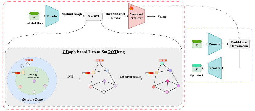
Overall framework of GROOT.
3.2. Constructing Latent Space of Protein Sequences
Unsupervised learning has achieved remarkable success in domains like natural language processing (Brown et al., 2020) and computer vision (Kirillov et al., 2023). This method efficiently learns data representations by identifying underlying patterns without requiring labeled data. The label-free nature of unsupervised learning aligns well with protein design challenges, where experimental fitness evaluations are costly, while unlabeled sequences are abundant. In this work, considering a dataset of unlabeled sequences of a protein family denoted as , we train a VAE comprising an encoder and a decoder . Each sequence is encoded into a low-dimensional vector . Subsequently, the mean and log-variance of the variational posterior approximation are computed from using two feed-forward networks, and . A latent vector is then sampled from the Gaussian distribution , and the decoder maps back to the reconstructed protein sequence . The training objective involves the cross-entropy loss between the ground truth sequence and the generated , as well as the Kullback-Leibler (KL) divergence between and :
| (2) |
Here, is the hyperparameter to control the disentanglement property of the VAE’s latent space. A critical distinction must be made between the latent space of protein sequences and the protein fitness landscape. While training a VAE-based model, we do not access protein fitness scores, but we learn their continuous representations. Consequently, this VAE-based model is trained on the entirety of available protein family sequences. Subsequently, labeled sequences are encoded by the pretrained VAE into -dimensional latent points, enabling the supervised training of a surrogate model, , to predict fitness values and approximate the fitness landscape.
3.2.1. VAE’s Architecture
We go into detail regarding the architecture of the VAE used in our study.
Encoder
incorporates a pre-trained ESM-2 (Lin et al., 2023) followed by a latent encoder to compute the latent representation . In our study, we leverage the powerful representation of the pre-trained 30-layer ESM-2 by making it the encoder of our model. Given an input sequence , where , ESM-2 computes representations for each token in , resulting in a token-level hidden representation . We calculate the global representation of via a weighted sum of its tokens:
| (3) |
here, is a learnable global attention vector. Then, two multi-layer perceptrons (MLPs) are used to compute and , where the latent dimension is . Finally, a latent representation is sampled from , which is further proceeded to the decoder to reconstruct the sequence .
Decoder
To decode latent points into sequences, we employ a deep convolutional network as proposed by Castro et al. (2022), consisting of four one-dimensional convolutional layers. ReLU activations and batch normalization layers are applied between the convolutional layers, except for the final layer.
3.3. Latent Graph-based Smoothing
Graph Construction
We need to build a graph from the sequences in to perform label propagation. Algorithm 1 demonstrates our algorithm to construct a kNN graph from the latent vectors . The graph’s nodes are created by sampling sequences , and the edges are constructed by -nearest neighbors to the latent embeddings of , where is the pre-trained encoder. We introduce new nodes to by interpolating the learned latent with random noise . We argue that Levenshtein distance is an inadequate metric for computing protein sequence similarity as done in (Kirjner et al., 2024) because marginal amino acid variations can result in substantial fitness disparities (Maynard Smith, 1970; Brookes et al., 2022b). Meanwhile, high-dimensional latent embeddings are effective at capturing implicit patterns within protein sequences. Consequently, Euclidean distance can serve as a suitable metric to quantify sequence similarity for constructing kNN graphs, as proteins with comparable properties (indicated by small fitness score differences) tend to cluster closely in the latent space. Algorithm 1 presents our graph construction pipeline.
Generating Pseudo-label
We consider a constructed graph G. For each node , we assign a fitness label , creating a set of fitness labels . This set can be further decomposed into , representing the known and unknown labels, respectively. Known labels are obtained from the training dataset, while unknown labels are initialized by 0 and assigned to randomly generated nodes, as shown in line 3 of Algorithm 2. We then run the following label propagation in times.
| (4) |
here, is a weighted coefficient and is a weighted adjacency matrix, defined as:
| (5) |
and is the Euclidean distance, is a controllable factor. In summary, Algorithm 2 details our smoothing strategy by label propagation.
3.4. Theoretical Justification
This section delves into the theoretical foundations of our proposed method. We begin by discussing the concepts of interpolation and extrapolation within high-dimensional latent embedding spaces. These concepts ensure the correctness of generating additional pseudo-samples within the latent space of a VAE-based model. Subsequently, leveraging the definition of convex hulls, we establish an upper bound for the expected distance between the generated nodes and the collection of training latent embeddings. This bound informs the intuition behind our kNN graph construction, detailed in Algorithm 1. Consequently, employing label propagation within this bounded distance emerges as a rational strategy for assigning pseudo-labels to the newly generated nodes.
We first list the definitions of a convex hull, interpolation, and extrapolation as follows:
Definition 3.1.
Let be a set of points in , a convex hull of is defined as:
Definition 3.2 (Balestriero et al. (2021)).
Interpolation occurs for a sample whenever this sample belongs to , if not, extrapolation occurs.
Assumptions
Given a set of training protein sequences , we use the encoder of the pretrained VAE to compute their latent embeddings, resulting in a set of latent vectors , where (see Section 3.2). In this paper, we consider the scenario wherein we have limited access to experimental data, and we train a VAE-based model to represent continuous -dimensional latent vectors of those available sequences. This, therefore, gives rise to two mild assumptions in our work.
-
•
Assumption 1: is significantly smaller than the exponential in , where represents the number of data samples.
-
•
Assumption 2: Each latent vector is sampled from . This is achieved by regularizing the model with divergence loss as shown in the Equation 2.
We assess GROOT’s extrapolation capabilities by computing the probability of its generated samples falling outside the convex hull of the training data within the latent space. Subsequently, we derive an upper bound for these reliable extrapolation regions. These findings are formalized in the following propositions.
Proposition 0.
Let be a set of i.i.d -dimensional samples from . Assume that and let for some , , and , then
We leave the proof of the presented proposition in Section A.1. Proposition 3.3 elucidates that in a limited data scenario (i.e. ), the probability for a synthetic latent node lying outside the convex hull of training set goes to 1 as the latent dimension grows. Based on Definition 3.2, this theoretical result guarantees the correctness of our formula shown in line 4 of Algorithm 1 in expanding the latent space of protein sequences. However, when generated nodes are located far from the training convex hull, their embedding vectors differ significantly from those in the training set. This disparity hinders the identification of meaningful similarities and can result in unreliable fitness scores determined through label propagation. This brings us to Proposition 3.4.
Proposition 0.
Let be a set of i.i.d -dimensional samples from . For any , we define with , the following holds:
where is the distance from a point to , and is the Euclidean distance.
The proof of this proposition can be found in Section A.2. Proposition 3.4 allows us to quantify the expected distance from a randomly generated node based on our formula to the available training set. The derived upper bound increases linearly w.r.t square root of the latent dimension with a rate of . It is worth noting that is used to control the exploration rate of our algorithm. As , the generated node closely resembles a training node . Conversely, a lower introduces more noise into the latent vectors, resulting in samples that are further from the source nodes. This upper bound ensures that synthetic nodes remain within a controllable ”reliable zone”, making label propagation a sensible choice, as the label values of these synthetic nodes cannot deviate too far from the overall distribution of existing nodes.
In summary, Propositions 3.3 and 3.4 offer theoretical underpinnings for our latent-based smoothing approach. By mapping discrete sequences to a continuous -dimensional latent space, we establish a quantitative relationship between newly added and original training nodes, governed by parameters and . This quantitative connection enhances the interpretability of our method.
3.5. Model-based Optimization Algorithm
Latent space model-based optimization (MBO) employs surrogate models, , to efficiently guide the search for optimal values that maximize expensive black-box functions. The effectiveness of MBO depends on the accuracy of the surrogate model as poorly trained surrogates can hinder the optimization process by providing misleading information. As shown in Algorithm 3, lines 1, 4, and 5 encompass the standard MBO process of encoding training vectors into latent space and training a surrogate model to predict fitness scores Y based on these embeddings. Meanwhile, lines 2 and 3 are two additional steps introduced by GROOT before surrogate training. GROOT is agnostic to domains as we can use any encoding method to compute latent embeddings of target domains. Moreover, GROOT can be used in tandem with any surrogate models as it only accesses the data representations. These two properties make GROOT a versatile approach for optimization tasks in a wide range of domains.
4. Experiments
We demonstrate the benefits of our proposed GROOT on two protein tasks with varying levels of label scarcity. Furthermore, since obtaining the ground-truth fitness of generated sequences is costly, we further evaluate our method on Design-Bench (Trabucco et al., 2022). These benchmarks have exact oracles, providing a better validation of our method’s performance on real-world datasets.
Design-Bench
Due to space constraints, we leave the presentation of tasks, baselines, evaluation metrics, and implementation details in Appendix F. Table 1 shows the performance of various methods across three Design-Bench tasks and their mean scores. While most methods perform well, GROOT achieves the highest average score in maximum performance and is slightly behind the SOTA baseline in median and mean benchmarks. Since these tasks are evaluated by an exact oracle and our performance is competitive with other SOTA methods, this confirms that our approach is effective on real-world data, enhancing the reliability of our work.
| Method | D’Kitty | Ant | TF Bind 8 | Mean | |
| Score | |||||
| Median | MINs | 0.86 (0.01) | 0.49 (0.15) | 0.42 (0.02) | 0.59 |
| BONET | 0.85 (0.01) | 0.60 (0.12) | 0.44 (0.00) | 0.63 | |
| BDI | 0.59 (0.02) | 0.40 (0.02) | 0.54 (0.03) | 0.51 | |
| ExPT | 0.90 (0.01) | 0.71 (0.02) | 0.47 (0.01) | 0.69 | |
| GROOT | 0.82 (0.01) | 0.62 (0.01) | 0.52 (0.01) | 0.65 | |
| Max | MINs | 0.93 (0.01) | 0.89 (0.01) | 0.81 (0.03) | 0.88 |
| BONET | 0.91 (0.01) | 0.84 (0.04) | 0.69 (0.15) | 0.81 | |
| BDI | 0.92 (0.01) | 0.81 (0.09) | 0.91 (0.07) | 0.88 | |
| ExPT | 0.97 (0.01) | 0.97 (0.00) | 0.93 (0.04) | 0.96 | |
| GROOT | 0.98 (0.01) | 0.97 (0.00) | 0.98 (0.02) | 0.98 | |
| Mean | MINs | 0.62 (0.03) | 0.01 (0.01) | 0.42 (0.03) | 0.35 |
| BONET | 0.84 (0.02) | 0.58 (0.02) | 0.45 (0.01) | 0.62 | |
| BDI | 0.57 (0.03) | 0.39 (0.01) | 0.54 (0.03) | 0.50 | |
| ExPT | 0.87 (0.02) | 0.64 (0.03) | 0.48 (0.01) | 0.66 | |
| GROOT | 0.78 (0.03) | 0.60 (0.01) | 0.55 (0.02) | 0.64 |
4.1. Experiment Setup
Datasets and Oracles
Following Kirjner et al. (2024), we evaluate our method on two proteins, GFP (Sarkisyan et al., 2016) and AAV (Bryant et al., 2021). The length is 237 for GFP and 28 for the functional segment of AAV. The full GFP dataset comprises 54,025 mutant sequences with associated log-fluorescence intensity, while the AAV dataset contains 44,156 sequences linked to their ability to package a DNA payload. The fitness values in both datasets are min-max normalized for evaluation but remain unchanged during training and inference. To demonstrate the advantages of our smoothing method, we use the harder1, harder2, and harder3 level benchmarks proposed by Kirjner et al. (2024) to sample training datasets for each task, simulating scenarios with scarce labeled data111Results of other difficulties are presented in the Appendix C. Table 2 provides statistics for each level benchmark. All methods, including baselines, start optimization using the entire training set and are evaluated on the best 128 generated sequences, with approximated fitness predicted by oracles provided by Kirjner et al. (2024). It is important to note that oracles do not participate in the optimization process and are only used as in-silico evaluators to validate final proposed designs of each method.
| Task | Difficulty | Fitness | Mutational | Best | |
| Range () | Gap | Fitness | |||
| AAV | Harder1 | th | |||
| Harder2 | th | ||||
| Harder3 | th | ||||
| GFP | Harder1 | th | |||
| Harder2 | th | ||||
| Harder3 | th |
| AAV harder1 task | AAV harder2 task | AAV harder3 task | |||||||
| Method | Fitness | Diversity | Novelty | Fitness | Diversity | Novelty | Fitness | Diversity | Novelty |
| AdaLead | 0.38 (0.0) | 5.5 (0.5) | 7.0 (0.7) | 0.43 (0.0) | 4.2 (0.7) | 7.8 (0.8) | 0.37 (0.0) | 6.22 (0.9) | 8.0 (1.2) |
| CbAS | 0.02 (0.0) | 22.9 (0.1) | 18.5 (0.5) | 0.01 (0.0) | 23.2 (0.1) | 19.3 (0.4) | 0.01 (0.0) | 23.2 (0.1) | 19.3 (0.4) |
| BO | 0.00 (0.0) | 20.4 (0.3) | 21.8 (0.4) | 0.01 (0.0) | 20.4 (0.0) | 22.0 (0.0) | 0.01 (0.0) | 20.6 (0.3) | 22.0 (0.0) |
| GFN-AL | 0.00 (0.0) | 15.4 (6.2) | 21.6 (0.5) | 0.00 (0.0) | 8.1 (3.5) | 21.6 (1.0) | 0.00 (0.0) | 7.6 (0.8) | 22.6 (1.4) |
| PEX | 0.23 (0.0) | 6.4 (0.5) | 3.8 (0.7) | 0.30 (0.0) | 7.8 (0.4) | 5.0 (0.0) | 0.26 (0.0) | 7.3 (0.7) | 4.4 (0.5) |
| GGS | 0.30 (0.0) | 13.6 (0.2) | 14.5 (0.3) | 0.27 (0.0) | 16.0 (0.0) | 19.4 (0.0) | 0.38 (0.0) | 7.0 (0.1) | 9.6 (0.1) |
| ReLSO | 0.15 (0.0) | 20.9 (0.0) | 13.0 (0.0) | 0.17 (0.0) | 20.3 (0.0) | 13.0 (0.0) | 0.22 (0.0) | 17.8 (0.0) | 11.0 (0.0) |
| S-ReLSO | 0.24 (0.0) | 11.5 (0.0) | 13.0 (0.0) | 0.28 (0.0) | 16.4 (0.0) | 6.5 (0.0) | 0.27 (0.0) | 17.7 (0.0) | 11.0 (0.0) |
| GROOT | 0.46 (0.1) | 9.8 (1.6) | 12.2 (0.5) | 0.45 (0.0) | 9.9 (0.8) | 13.0 (0.0) | 0.42 (0.1) | 11.0 (2.0) | 13.0 (0.0) |
| GFP harder1 task | GFP harder2 task | GFP harder3 task | |||||||
| Method | Fitness | Diversity | Novelty | Fitness | Diversity | Novelty | Fitness | Diversity | Novelty |
| AdaLead | 0.39 (0.0) | 8.4 (3.2) | 9.0 (1.2) | 0.4 (0.0) | 7.3 (2.8) | 9.8 (0.4) | 0.42 (0.0) | 6.4 (2.3) | 9.0 (1.2) |
| CbAS | -0.08 (0.0) | 172.2 (35.7) | 201.5 (1.5) | -0.09 (0.0) | 158.4 (34.8) | 202.0 (0.7) | -0.08 (0.0) | 186.4 (33.4) | 201.5 (0.9) |
| BO | -0.08 (0.1) | 58.9 (1.9) | 192.3 (11.3) | -0.04 (0.1) | 57.1 (1.7) | 192.3 (11.3) | -0.07 (0.1) | 57.8 (2.2) | 177.9 (41.2) |
| GFN-AL | 0.21 (0.1) | 74.3 (55.3) | 219.2 (3.3) | 0.14 (0.2) | 27.0 (9.5) | 223.5 (2.4) | 0.21 (0.0) | 37.5 (21.7) | 219.8 (4.3) |
| PEX | 0.13 (0.0) | 12.6 (1.2) | 7.1 (1.1) | 0.17 (0.0) | 12.6 (1.2) | 7.1 (1.1) | 0.19 (0.0) | 12.2 (1.1) | 7.8 (1.7) |
| GGS | 0.67 (0.0) | 4.7 (0.2) | 9.1 (0.1) | 0.60 (0.0) | 5.4 (0.2) | 9.8 (0.1) | 0.00 (0.0) | 15.7 (0.4) | 19.0 (2.2) |
| ReLSO | 0.94 (0.0)† | 0.0 (0.0) | 8.0 (0.0) | 0.94 (0.0)† | 0.0 (0.0) | 8.0 (0.0) | 0.94 (0.0)† | 0.0 (0.0) | 8.0 (0.0) |
| S-ReLSO | 0.94 (0.0)† | 0.0 (0.0) | 8.0 (0.0) | 0.94 (0.0)† | 0.0 (0.0) | 8.0 (0.0) | 0.94 (0.0)† | 0.0 (0.0) | 8.0 (0.0) |
| GROOT | 0.88 (0.0) | 3.0 (0.2) | 7.0 (0.0) | 0.87 (0.0) | 3.0 (0.1) | 7.5 (0.5) | 0.62 (0.2) | 7.6 (1.5) | 8.6 (1.5) |
| indicates that the generated population has collapsed (i.e., producing only a single sequence). | |||||||||
Baselines
We evaluate our method against several representative baselines using the open-source toolkit FLEXS (Sinai et al., 2020): AdaLead (Sinai et al., 2020), CbAS (Brookes et al., 2019), and Bayesian Optimization (BO) (Wilson et al., 2017). In addition to these algorithms, we also benchmark against some most recent methods: GFN-AL (Jain et al., 2022), ReLSO (Castro et al., 2022), PEX (Ren et al., 2022), and GGS (Kirjner et al., 2024), utilizing and modifying the code provided by their respective authors. Furthermore, we assess ReLSO enhanced with our smoothing strategy for better optimization, termed S-ReLSO.
Evaluation Metrics
We use three metrics proposed by Jain et al. (2022): fitness, diversity, and novelty. Let the optimized sequences . Fitness is defined as the median of the evaluated fitness of proposed designs. Diversity is the median of the distances between every pair of sequences in . Novelty is defined as the median of the distances between every generated sequences to the training set. Mathematical definitions of these metrics are defined in the Appendix B.
Implementation Details
For each task, we use the full dataset to train the VAE, whose architecture has been described in Section 3.2. We utilize the pretrained checkpoint esm2_t30_150M_UR50D222https://huggingface.co/facebook/esm2_t30_150M_UR50D of the ESM-2 model, fine-tuning only the last layer while freezing the rest. The latent representation space dimension is set to . For the latent graph-based smoothing, we set the number of nodes to , label propagation’s coefficient to , controller factor to , the number of propagation layers to , and the number of neighbors to . It is important to note that these hyperparameters are not finely tuned. The hyperparameter tuning process is described in the Appendix E. After the smoothing process, the features and refined labels are inputted into a surrogate model, specifically a shallow 2-layer multi-layers perceptron (MLP) with a dropout rate of in the first layer, to train a smoothed surrogate model. Despite its simplicity, we consider MLP a suitable choice due to its proven effectiveness in previous studies (Huang et al., 2021). For model-based optimization, we select two gradient-based algorithms to exploit the smoothness of the surrogate model: Gradient Ascent (GA) with a learning rate of for iterations and Limited-memory Broyden-Fletcher-Goldfarb-Shanno (L-BFGS) (Liu and Nocedal, 1989) for a maximum of iterations. While various optimization algorithms are available, we choose these gradient-based methods based on the premise that they can effectively leverage the smoothness of the surrogate model. It is crucial to note that our primary focus is not on evaluating multiple optimization methods, but rather on demonstrating the effectiveness of the smoothing strategy. We empirically evaluate these two algorithms and report the best results.
4.2. Numerical Results
We report the mean and standard deviation of the evaluation metrics over five runs with different random seeds in Table 3. Firstly, compared to the best fitness of the training data (Table 2), our method successfully optimizes all tasks. For AAV tasks, our method achieves SOTA results across all difficulty levels. Notably, although our method only slightly exceeds AdaLead in the harder2 task, GROOT generates sequences whose novelty falls within the mutation gap range, indicating appropriate extrapolation and a higher likelihood of producing synthesizable proteins. Additionally, applying our smoothing strategy to ReLSO improves the model’s performance by in the harder1, in the harder2, and in the harder3 tasks. For GFP tasks, GROOT outperforms all baseline methods across all difficulties, especially in the harder3 difficulty, where GGS failed to optimize properly. It is crucial to mention that ReLSO failed to generate diverse sequences in GFP tasks, as indicated by zero diversity across five different runs. Overall, we observe that GROOT achieves the highest fitness while maintaining respectable diversity and novelty.
4.3. Analysis
Impact of smoothing on extrapolation and general performance
For each benchmark, we assess the impact of smoothing on extrapolation capabilities by measuring the Mean Absolute Error (MAE) of the surrogate model on the benchmark’s training and holdout datasets relative to the experimental ground-truth. Table 4 shows the benefits of smoothing on extrapolation to held out ground-truth experimental data. Our results demonstrate that smoothing reduces MAE for both the training and holdout sets. This reduction occurs because our smoothing strategy acts as a data augmentation technique in the latent space, enhancing the robustness of the supervised model. We also observe that the MAE for both sets increases gradually as the task becomes more difficult. We hypothesize that this is due to the smaller training set size in more difficult tasks, requiring a greater number of new samples to construct a graph. While the labels of these new samples are not exact, they help to smooth the latent landscape, resulting in a smoother but not perfectly accurate surrogate model, which in turn increases the MAE.
Additionally, Table 5 demonstrates how a smoothed model dramatically outperforms its unsmoothed counterpart across all tasks. For AAV, the results show up to a threefold improvement compared to the unsmoothed surrogate model. For GFP, without smoothing, the optimization algorithm struggles to find a maximum point, resulting in suboptimal performance. With our smoothing technique, the optimization algorithm can optimize properly. Our findings indicate that our smoothing strategy enables gradient-based optimization methods to better navigate the search space and identify superior maxima. However, we also observe that applying smoothing decreases diversity. This can be explained by the optimization process converging, causing the population to concentrate in certain high-fitness regions. In contrast, without proper optimization, the population diverges and spreads throughout the search space.
| Task | Difficulty | Smoothed | Train | Holdout |
| MAE | MAE | |||
| AAV | Harder1 | No | 4.94 | 8.93 |
| Yes | 1.02 | 5.78 | ||
| Harder2 | No | 4.67 | 8.91 | |
| Yes | 1.10 | 6.11 | ||
| Harder3 | No | 4.13 | 8.87 | |
| Yes | 1.44 | 7.30 | ||
| GFP | Harder1 | No | 1.39 | 2.81 |
| Yes | 0.22 | 1.71 | ||
| Harder2 | No | 1.34 | 2.81 | |
| Yes | 0.31 | 1.85 | ||
| Harder3 | No | 1.33 | 2.80 | |
| Yes | 0.51 | 2.09 |
| Task | Difficulty | Smoothed | Fitness | Diversity | Novelty |
| AAV | Harder1 | No | 0.12 | 20.0 | 10.0 |
| Yes | 0.46 | 9.8 | 12.2 | ||
| Harder2 | No | 0.11 | 20.0 | 9.6 | |
| Yes | 0.45 | 9.9 | 13.0 | ||
| Harder3 | No | 0.12 | 20.1 | 10.0 | |
| Yes | 0.42 | 11.0 | 13.0 | ||
| GFP | Harder1 | No | -0.12 | 71.0 | 42.2 |
| Yes | 0.88 | 3.0 | 7.0 | ||
| Harder2 | No | -0.18 | 69.5 | 41.1 | |
| Yes | 0.87 | 3.0 | 7.5 | ||
| Harder3 | No | -0.17 | 64.0 | 37.0 | |
| Yes | 0.62 | 7.6 | 8.6 |
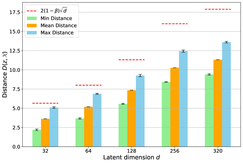
Distance from generated nodes outside the convex hull to the set of training nodes.
Empirical analysis of our propositions
In this section, we directly validate our proposed Propositions 3.3 and 3.4 through experiments. Firstly, we train multiple VAEs with the same architecture described in Section 3.2, modifying only the latent dimension size . For each VAE version, we construct a graph and apply the smoothing technique as described in Section 3.3 to generate new nodes. Secondly, to determine whether the generated nodes lie within the convex hull, we check if each point can be expressed as a convex combination of the training points. This is formulated as a linear programming problem and can be easily solved using existing libraries333https://docs.scipy.org/doc/scipy/reference/generated/scipy.optimize.linprog.html. After identifying the number of nodes lying outside the convex hull, we calculate the Euclidean distance between the outside nodes and the set of training nodes.
We validate our propositions on the GFP harder3 task, setting consistently across all runs to maintain a constant upper bound. Our experiments reveal that, regardless of dimensional size, 100% of the synthetic nodes lie outside the convex hull. Figure 2 demonstrates distance calculations between the outside nodes and the set of training nodes. It is evident that although the distance increases with the latent dimension, none of the generated nodes in any VAE versions exceed the proven upper bound. This demonstrates that our smoothing technique can expand into extrapolation regions while remaining within a suitable range, avoiding distances too far from the training set that could introduce errors in surrogate model predictions.
Explore the limits of smoothing strategy
In this section, we investigate the smoothing capabilities of our method by testing its limits. We use the GFP harder3 task and the AAV harder3 task as examined cases, further subsampling the dataset with ratios in two different ways, namely: random and lowest. In the random setting, data points are randomly subsampled with the given ratio , while in the lowest setting, we use the fraction of the dataset with the lowest fitness scores.
Using the same hyperparameters, Figure 3 shows the median performance of GROOT on AAV and GFP w.r.t the ratio in both settings. In the random setting, our method outperforms the best data point in the entire harder3 dataset using only of the labeled data, which amounts to fewer than samples per set. In the lowest setting, the method requires of the labeled data, approximately samples per set, to achieve similar performance. This demonstrates that our method is effective even under extreme conditions with limited labeled data.
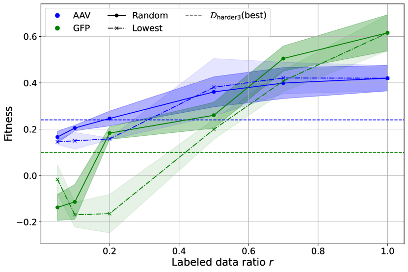
Performance when varying the training data ratio .
5. Conclusion
This paper presents a novel method, GROOT, to address the scarcity of labeled data in practical protein sequence design. GROOT embeds protein sequences into a continuous latent space. In this space, we generate additional synthetic latent points by interpolating existing data points and Gaussian noise and estimating their fitness scores using label propagation. We provide theoretical underpinnings based on convex hull and extrapolation to support GROOT’s efficacy. Experimental results confirm the method’s effectiveness in protein design under extreme labeled data-limited conditions.
Limitations
Our proposed method, GROOT, has some limitations on hyperparameters. These numbers are sensitive to landscape characteristics, and one should search for their optimal values when optimizing new landscapes. We have detailed the hyperparameter tuning process in Appendix E and found that, despite some sensitivity differences between datasets, the optimal hyperparameters remain relatively stable across multiple difficulty levels within the same landscape, thereby reducing the burden of searching for optimal settings. Additionally, we theoretically characterize the relationship between GROOT’s hyperparameters and the sampled nodes, guaranteeing controllability over the entire framework. A promising extension of GROOT is to find better ways to determine the optimal value of , which can be done by analyzing the effect of random mutations on each family of protein sequences.
References
- (1)
- Ahn et al. (2020) Michael Ahn, Henry Zhu, Kristian Hartikainen, Hugo Ponte, Abhishek Gupta, Sergey Levine, and Vikash Kumar. 2020. ROBEL: Robotics Benchmarks for Learning with Low-Cost Robots. In Proceedings of the Conference on Robot Learning (Proceedings of Machine Learning Research, Vol. 100), Leslie Pack Kaelbling, Danica Kragic, and Komei Sugiura (Eds.). PMLR, 1300–1313. https://proceedings.mlr.press/v100/ahn20a.html
- Akiba et al. (2019) Takuya Akiba, Shotaro Sano, Toshihiko Yanase, Takeru Ohta, and Masanori Koyama. 2019. Optuna: A Next-generation Hyperparameter Optimization Framework. In Proceedings of the 25th ACM SIGKDD International Conference on Knowledge Discovery & Data Mining (Anchorage, AK, USA) (KDD ’19). Association for Computing Machinery, New York, NY, USA, 2623–2631. https://doi.org/10.1145/3292500.3330701
- Arnold (1996) Frances H. Arnold. 1996. Directed evolution: Creating biocatalysts for the future. Chemical Engineering Science 51, 23 (1996), 5091–5102. https://doi.org/10.1016/S0009-2509(96)00288-6
- Arnold (2018) Frances H. Arnold. 2018. Directed Evolution: Bringing New Chemistry to Life. Angewandte Chemie International Edition 57, 16 (2018), 4143–4148. https://doi.org/10.1002/anie.201708408 arXiv:https://onlinelibrary.wiley.com/doi/pdf/10.1002/anie.201708408
- Balestriero et al. (2021) Randall Balestriero, Jerome Pesenti, and Yann LeCun. 2021. Learning in high dimension always amounts to extrapolation. arXiv preprint arXiv:2110.09485 (2021).
- Brockman et al. (2016) Greg Brockman, Vicki Cheung, Ludwig Pettersson, Jonas Schneider, John Schulman, Jie Tang, and Wojciech Zaremba. 2016. OpenAI Gym. arXiv:1606.01540 [cs.LG] https://arxiv.org/abs/1606.01540
- Brookes et al. (2019) David Brookes, Hahnbeom Park, and Jennifer Listgarten. 2019. Conditioning by adaptive sampling for robust design. In Proceedings of the 36th International Conference on Machine Learning (Proceedings of Machine Learning Research, Vol. 97), Kamalika Chaudhuri and Ruslan Salakhutdinov (Eds.). PMLR, 773–782. https://proceedings.mlr.press/v97/brookes19a.html
- Brookes et al. (2022a) David H. Brookes, Amirali Aghazadeh, and Jennifer Listgarten. 2022a. On the sparsity of fitness functions and implications for learning. Proceedings of the National Academy of Sciences 119, 1 (2022), e2109649118. https://doi.org/10.1073/pnas.2109649118 arXiv:https://www.pnas.org/doi/pdf/10.1073/pnas.2109649118
- Brookes et al. (2022b) David H Brookes, Amirali Aghazadeh, and Jennifer Listgarten. 2022b. On the sparsity of fitness functions and implications for learning. Proceedings of the National Academy of Sciences 119, 1 (2022), e2109649118.
- Brown et al. (2020) Tom Brown, Benjamin Mann, Nick Ryder, Melanie Subbiah, Jared D Kaplan, Prafulla Dhariwal, Arvind Neelakantan, Pranav Shyam, Girish Sastry, Amanda Askell, Sandhini Agarwal, Ariel Herbert-Voss, Gretchen Krueger, Tom Henighan, Rewon Child, Aditya Ramesh, Daniel Ziegler, Jeffrey Wu, Clemens Winter, Chris Hesse, Mark Chen, Eric Sigler, Mateusz Litwin, Scott Gray, Benjamin Chess, Jack Clark, Christopher Berner, Sam McCandlish, Alec Radford, Ilya Sutskever, and Dario Amodei. 2020. Language Models are Few-Shot Learners. In Advances in Neural Information Processing Systems, H. Larochelle, M. Ranzato, R. Hadsell, M.F. Balcan, and H. Lin (Eds.), Vol. 33. Curran Associates, Inc., 1877–1901. https://proceedings.neurips.cc/paper_files/paper/2020/file/1457c0d6bfcb4967418bfb8ac142f64a-Paper.pdf
- Bryant et al. (2021) Drew H. Bryant, Ali Bashir, Sam Sinai, Nina K. Jain, Pierce J. Ogden, Patrick F. Riley, George M. Church, Lucy J. Colwell, and Eric D. Kelsic. 2021. Deep diversification of an AAV capsid protein by machine learning. Nature Biotechnology 39, 6 (01 Jun 2021), 691–696. https://doi.org/10.1038/s41587-020-00793-4
- Castro et al. (2022) Egbert Castro, Abhinav Godavarthi, Julian Rubinfien, Kevin Givechian, Dhananjay Bhaskar, and Smita Krishnaswamy. 2022. Transformer-based protein generation with regularized latent space optimization. Nature Machine Intelligence 4, 10 (01 Oct 2022), 840–851. https://doi.org/10.1038/s42256-022-00532-1
- Chandrasekaran et al. (2012) Venkat Chandrasekaran, Benjamin Recht, Pablo A Parrilo, and Alan S Willsky. 2012. The convex geometry of linear inverse problems. Foundations of Computational mathematics 12, 6 (2012), 805–849.
- Chen et al. (2022) Can Chen, Yingxueff Zhang, Jie Fu, Xue (Steve) Liu, and Mark Coates. 2022. Bidirectional Learning for Offline Infinite-width Model-based Optimization. In Advances in Neural Information Processing Systems, S. Koyejo, S. Mohamed, A. Agarwal, D. Belgrave, K. Cho, and A. Oh (Eds.), Vol. 35. Curran Associates, Inc., 29454–29467. https://proceedings.neurips.cc/paper_files/paper/2022/file/bd391cf5bdc4b63674d6da3edc1bde0d-Paper-Conference.pdf
- Chen et al. (2023) Tianlai Chen, Pranay Vure, Rishab Pulugurta, and Pranam Chatterjee. 2023. AMP-Diffusion: Integrating Latent Diffusion with Protein Language Models for Antimicrobial Peptide Generation. In NeurIPS 2023 Generative AI and Biology (GenBio) Workshop. https://openreview.net/forum?id=145TM9VQhx
- Emami et al. (2023) Patrick Emami, Aidan Perreault, Jeffrey Law, David Biagioni, and Peter St. John. 2023. Plug and play directed evolution of proteins with gradient-based discrete MCMC. Machine Learning: Science and Technology 4, 2 (April 2023), 025014. https://doi.org/10.1088/2632-2153/accacd
- Fowler and Fields (2014) Douglas M. Fowler and Stanley Fields. 2014. Deep mutational scanning: a new style of protein science. Nature Methods 11, 8 (01 Aug 2014), 801–807. https://doi.org/10.1038/nmeth.3027
- Frey et al. (2024) Nathan C. Frey, Dan Berenberg, Karina Zadorozhny, Joseph Kleinhenz, Julien Lafrance-Vanasse, Isidro Hotzel, Yan Wu, Stephen Ra, Richard Bonneau, Kyunghyun Cho, Andreas Loukas, Vladimir Gligorijevic, and Saeed Saremi. 2024. Protein Discovery with Discrete Walk-Jump Sampling. In The Twelfth International Conference on Learning Representations. https://openreview.net/forum?id=zMPHKOmQNb
- Gómez-Bombarelli et al. (2018) Rafael Gómez-Bombarelli, Jennifer N. Wei, David Duvenaud, José Miguel Hernández-Lobato, Benjamín Sánchez-Lengeling, Dennis Sheberla, Jorge Aguilera-Iparraguirre, Timothy D. Hirzel, Ryan P. Adams, and Alán Aspuru-Guzik. 2018. Automatic Chemical Design Using a Data-Driven Continuous Representation of Molecules. ACS Central Science 4, 2 (2018), 268–276. https://doi.org/10.1021/acscentsci.7b00572 arXiv:https://doi.org/10.1021/acscentsci.7b00572 PMID: 29532027.
- Huang et al. (2016) Po-Ssu Huang, Scott E. Boyken, and David Baker. 2016. The coming of age of de novo protein design. Nature 537, 7620 (01 Sep 2016), 320–327. https://doi.org/10.1038/nature19946
- Huang et al. (2021) Qian Huang, Horace He, Abhay Singh, Ser-Nam Lim, and Austin Benson. 2021. Combining Label Propagation and Simple Models out-performs Graph Neural Networks. In International Conference on Learning Representations. https://openreview.net/forum?id=8E1-f3VhX1o
- Jain et al. (2022) Moksh Jain, Emmanuel Bengio, Alex Hernandez-Garcia, Jarrid Rector-Brooks, Bonaventure F. P. Dossou, Chanakya Ajit Ekbote, Jie Fu, Tianyu Zhang, Michael Kilgour, Dinghuai Zhang, Lena Simine, Payel Das, and Yoshua Bengio. 2022. Biological Sequence Design with GFlowNets. In Proceedings of the 39th International Conference on Machine Learning (Proceedings of Machine Learning Research, Vol. 162), Kamalika Chaudhuri, Stefanie Jegelka, Le Song, Csaba Szepesvari, Gang Niu, and Sivan Sabato (Eds.). PMLR, 9786–9801. https://proceedings.mlr.press/v162/jain22a.html
- Kauffman and Weinberger (1989) Stuart A. Kauffman and Edward D. Weinberger. 1989. The NK model of rugged fitness landscapes and its application to maturation of the immune response. Journal of Theoretical Biology 141, 2 (Nov. 1989), 211–245. https://doi.org/10.1016/s0022-5193(89)80019-0
- Kirillov et al. (2023) Alexander Kirillov, Eric Mintun, Nikhila Ravi, Hanzi Mao, Chloe Rolland, Laura Gustafson, Tete Xiao, Spencer Whitehead, Alexander C. Berg, Wan-Yen Lo, Piotr Dollár, and Ross Girshick. 2023. Segment Anything. arXiv:2304.02643 (2023).
- Kirjner et al. (2024) Andrew Kirjner, Jason Yim, Raman Samusevich, Shahar Bracha, Tommi S. Jaakkola, Regina Barzilay, and Ila R Fiete. 2024. Improving protein optimization with smoothed fitness landscapes. In The Twelfth International Conference on Learning Representations. https://openreview.net/forum?id=rxlF2Zv8x0
- Kumar and Levine (2020) Aviral Kumar and Sergey Levine. 2020. Model Inversion Networks for Model-Based Optimization. In Advances in Neural Information Processing Systems, H. Larochelle, M. Ranzato, R. Hadsell, M.F. Balcan, and H. Lin (Eds.), Vol. 33. Curran Associates, Inc., 5126–5137. https://proceedings.neurips.cc/paper_files/paper/2020/file/373e4c5d8edfa8b74fd4b6791d0cf6dc-Paper.pdf
- Lee et al. (2023) Minji Lee, Luiz Felipe Vecchietti, Hyunkyu Jung, Hyunjoo Ro, Meeyoung Cha, and Ho Min Kim. 2023. Protein Sequence Design in a Latent Space via Model-based Reinforcement Learning. https://openreview.net/forum?id=OhjGzRE5N6o
- Lee et al. (2024) Minji Lee, Luiz Felipe Vecchietti, Hyunkyu Jung, Hyun Joo Ro, Meeyoung Cha, and Ho Min Kim. 2024. Robust Optimization in Protein Fitness Landscapes Using Reinforcement Learning in Latent Space. In Forty-first International Conference on Machine Learning. https://openreview.net/forum?id=0zbxwvJqwf
- Lin et al. (2023) Zeming Lin, Halil Akin, Roshan Rao, Brian Hie, Zhongkai Zhu, Wenting Lu, Nikita Smetanin, Robert Verkuil, Ori Kabeli, Yaniv Shmueli, Allan dos Santos Costa, Maryam Fazel-Zarandi, Tom Sercu, Salvatore Candido, and Alexander Rives. 2023. Evolutionary-scale prediction of atomic-level protein structure with a language model. Science 379, 6637 (2023), 1123–1130. https://doi.org/10.1126/science.ade2574 arXiv:https://www.science.org/doi/pdf/10.1126/science.ade2574
- Liu and Nocedal (1989) Dong C. Liu and Jorge Nocedal. 1989. On the limited memory BFGS method for large scale optimization. Mathematical Programming 45, 1 (01 Aug 1989), 503–528. https://doi.org/10.1007/BF01589116
- Mashkaria et al. (2023) Satvik Mehul Mashkaria, Siddarth Krishnamoorthy, and Aditya Grover. 2023. Generative Pretraining for Black-Box Optimization. In Proceedings of the 40th International Conference on Machine Learning (Proceedings of Machine Learning Research, Vol. 202), Andreas Krause, Emma Brunskill, Kyunghyun Cho, Barbara Engelhardt, Sivan Sabato, and Jonathan Scarlett (Eds.). PMLR, 24173–24197. https://proceedings.mlr.press/v202/mashkaria23a.html
- Maynard Smith (1970) John Maynard Smith. 1970. Natural Selection and the Concept of a Protein Space. Nature 225, 5232 (Feb. 1970), 563–564. https://doi.org/10.1038/225563a0
- Nguyen et al. (2023) Tung Nguyen, Sudhanshu Agrawal, and Aditya Grover. 2023. ExPT: Synthetic Pretraining for Few-Shot Experimental Design. In Advances in Neural Information Processing Systems, A. Oh, T. Naumann, A. Globerson, K. Saenko, M. Hardt, and S. Levine (Eds.), Vol. 36. Curran Associates, Inc., 45856–45869. https://proceedings.neurips.cc/paper_files/paper/2023/file/8fab4407e1fe9006b39180525c0d323c-Paper-Conference.pdf
- Qiu and Wei (2022) Yuchi Qiu and Guo-Wei Wei. 2022. CLADE 2.0: Evolution-Driven Cluster Learning-Assisted Directed Evolution. Journal of Chemical Information and Modeling 62, 19 (Sept. 2022), 4629–4641. https://doi.org/10.1021/acs.jcim.2c01046
- Raghavan et al. (2007) Usha Nandini Raghavan, Réka Albert, and Soundar Kumara. 2007. Near linear time algorithm to detect community structures in large-scale networks. Phys. Rev. E 76 (Sep 2007), 036106. Issue 3. https://doi.org/10.1103/PhysRevE.76.036106
- Ren et al. (2022) Zhizhou Ren, Jiahan Li, Fan Ding, Yuan Zhou, Jianzhu Ma, and Jian Peng. 2022. Proximal Exploration for Model-guided Protein Sequence Design. In Proceedings of the 39th International Conference on Machine Learning (Proceedings of Machine Learning Research, Vol. 162), Kamalika Chaudhuri, Stefanie Jegelka, Le Song, Csaba Szepesvari, Gang Niu, and Sivan Sabato (Eds.). PMLR, 18520–18536. https://proceedings.mlr.press/v162/ren22a.html
- Sarkisyan et al. (2016) Karen S. Sarkisyan, Dmitry A. Bolotin, Margarita V. Meer, Dinara R. Usmanova, Alexander S. Mishin, George V. Sharonov, Dmitry N. Ivankov, Nina G. Bozhanova, Mikhail S. Baranov, Onuralp Soylemez, Natalya S. Bogatyreva, Peter K. Vlasov, Evgeny S. Egorov, Maria D. Logacheva, Alexey S. Kondrashov, Dmitry M. Chudakov, Ekaterina V. Putintseva, Ilgar Z. Mamedov, Dan S. Tawfik, Konstantin A. Lukyanov, and Fyodor A. Kondrashov. 2016. Local fitness landscape of the green fluorescent protein. Nature 533, 7603 (01 May 2016), 397–401. https://doi.org/10.1038/nature17995
- Sinai et al. (2020) Sam Sinai, Richard Wang, Alexander Whatley, Stewart Slocum, Elina Locane, and Eric D. Kelsic. 2020. AdaLead: A simple and robust adaptive greedy search algorithm for sequence design. CoRR abs/2010.02141 (2020). arXiv:2010.02141 https://arxiv.org/abs/2010.02141
- Stanton et al. (2022) Samuel Stanton, Wesley Maddox, Nate Gruver, Phillip Maffettone, Emily Delaney, Peyton Greenside, and Andrew Gordon Wilson. 2022. Accelerating Bayesian Optimization for Biological Sequence Design with Denoising Autoencoders. In Proceedings of the 39th International Conference on Machine Learning (Proceedings of Machine Learning Research, Vol. 162), Kamalika Chaudhuri, Stefanie Jegelka, Le Song, Csaba Szepesvari, Gang Niu, and Sivan Sabato (Eds.). PMLR, 20459–20478. https://proceedings.mlr.press/v162/stanton22a.html
- Trabucco et al. (2022) Brandon Trabucco, Xinyang Geng, Aviral Kumar, and Sergey Levine. 2022. Design-Bench: Benchmarks for Data-Driven Offline Model-Based Optimization. In Proceedings of the 39th International Conference on Machine Learning (Proceedings of Machine Learning Research, Vol. 162), Kamalika Chaudhuri, Stefanie Jegelka, Le Song, Csaba Szepesvari, Gang Niu, and Sivan Sabato (Eds.). PMLR, 21658–21676. https://proceedings.mlr.press/v162/trabucco22a.html
- Trabucco et al. (2021) Brandon Trabucco, Aviral Kumar, Xinyang Geng, and Sergey Levine. 2021. Conservative Objective Models for Effective Offline Model-Based Optimization. In Proceedings of the 38th International Conference on Machine Learning (Proceedings of Machine Learning Research, Vol. 139), Marina Meila and Tong Zhang (Eds.). PMLR, 10358–10368. https://proceedings.mlr.press/v139/trabucco21a.html
- Tran and Hy (2024) Thanh V. T. Tran and Truong Son Hy. 2024. Protein Design by Directed Evolution Guided by Large Language Models. bioRxiv (2024). https://doi.org/10.1101/2023.11.28.568945 arXiv:https://www.biorxiv.org/content/early/2024/05/02/2023.11.28.568945.full.pdf
- Wang et al. (2021) Yajie Wang, Pu Xue, Mingfeng Cao, Tianhao Yu, Stephan T. Lane, and Huimin Zhao. 2021. Directed Evolution: Methodologies and Applications. Chemical Reviews 121, 20 (2021), 12384–12444. https://doi.org/10.1021/acs.chemrev.1c00260 arXiv:https://doi.org/10.1021/acs.chemrev.1c00260 PMID: 34297541.
- Wilson et al. (2017) James T. Wilson, Riccardo Moriconi, Frank Hutter, and Marc Peter Deisenroth. 2017. The reparameterization trick for acquisition functions. arXiv:1712.00424 [stat.ML] https://arxiv.org/abs/1712.00424
- Zhou et al. (2003) Dengyong Zhou, Olivier Bousquet, Thomas Lal, Jason Weston, and Bernhard Schölkopf. 2003. Learning with Local and Global Consistency. In Advances in Neural Information Processing Systems, S. Thrun, L. Saul, and B. Schölkopf (Eds.), Vol. 16. MIT Press. https://proceedings.neurips.cc/paper_files/paper/2003/file/87682805257e619d49b8e0dfdc14affa-Paper.pdf
Appendix A Proofs
A.1. Proof of Proposition 3.3
Proof.
We compute the probability that belongs to , . By definition, we have
Since , without loss of generality, let . The other cases can be computed similar, taking the mean gives the same results.
This will lead to
Since all are independent, for , we have:
Note that where . From here, since is large, we consider Chi-square as the normal approximations
We consider the two distribution
Since are all normal, and are also normal. Moreover,
and the variances are
Due to symmetric distribution of , we can see that . Moreover, and are independent random vectors, thus and are also independent, thus . From these deductions, we have shown that
Since iff , we derive that
Finally, we get that
Thus for all and sufficiently large, we have
In other words,
∎
A.2. Proof of Proposition 3.4
Proof.
Since , for any , we should have:
Replace by , we obtain:
We have that and . Chandrasekaran et al. (2012) has shown that the upper bound of their expectations’ norms is . Thus, we have
Therefore,
which completes the proof. ∎
Appendix B Evaluation Metrics
We provide mathematical definitions for each metric. Note that is the evaluator provided by Kirjner et al. (2024) to predict approximate fitness, serving as a proxy for experimental validation.
-
•
(Normalized) Fitness = where is the min-max normalized fitness based on the lowest and highest known fitness in .
-
•
Diversity = is the average sample similarity.
-
•
Novelty = where
is the minimum distance of sample to any of the starting sequences .
Appendix C Numerical Results For Other Protein Tasks
In this section, we present experimental results of other difficulties of two protein datasets: GFP and AAV. Table 6 provides statistics for each level benchmark. We use the same settings as described in Section 4.1 for this evaluation. Table 7 outlined the results of baselines and our GROOT. Although our method is designed for scenarios with limited labeled data, it achieves state-of-the-art (SOTA) results across all difficulty levels in both datasets. Additionally, the enhanced version of ReLSO incorporating our smoothing strategy, S-ReLSO, outperforms the original version by a significant margin in all tasks, particularly in the GFP medium task, where an 8-fold improvement is observed. These results demonstrate the effectiveness of our framework.
| Task | Difficulty | Fitness | Mutational | Best | |
| Range () | Gap | Fitness | |||
| AAV | Easy | th | |||
| Medium | th | ||||
| Hard | th | ||||
| GFP | Easy | th | |||
| Medium | th | ||||
| Hard | th |
| AAV easy task | AAV medium task | AAV hard task | |||||||
| Method | Fitness | Diversity | Novelty | Fitness | Diversity | Novelty | Fitness | Diversity | Novelty |
| AdaLead | 0.53 (0.0) | 5.7 (0.4) | 3.0 (0.7) | 0.49 (0.0) | 5.3 (0.7) | 6.3 (0.4) | 0.46 (0.0) | 5.4 (1.7) | 6.9 (0.9) |
| CbAS | 0.03 (0.0) | 23.2 (0.2) | 17.5 (0.5) | 0.02 (0.0) | 23.1 (0.1) | 18.3 (0.4) | 0.02 (0.0) | 23.0 (0.2) | 18.5 (0.5) |
| BO | 0.01 (0.0) | 20.1 (0.5) | 22.3 (0.4) | 0.00 (0.0) | 20.4 (0.2) | 21.5 (0.5) | 0.01 (0.0) | 20.5 (0.2) | 20.8 (0.4) |
| GFN-AL | 0.05 (0.0) | 18.2 (3.3) | 21.0 (0.0) | 0.01 (0.0) | 16.9 (2.4) | 21.4 (1.0) | 0.01 (0.0) | 14.4 (6.2) | 21.6 (0.5) |
| PEX | 0.44 (0.0) | 6.33 (1.1) | 4.0 (0.6) | 0.35 (0.0) | 6.86 (0.9) | 4.2 (1.0) | 0.29 (0.0) | 6.43 (0.5) | 3.8 (0.7) |
| GGS | 0.49 (0.0) | 9.0 (0.2) | 8.0 (0.0) | 0.51 (0.0) | 4.9 (0.2) | 5.4 (0.5) | 0.60 (0.0) | 4.5 (0.5) | 7.0 (0.0) |
| ReLSO | 0.18 (0.0) | 1.4 (0.0) | 5.0 (0.0) | 0.18 (0.0) | 15.7 (0.0) | 11.0 (0.0) | 0.03 (0.0) | 18.6 (0.0) | 15.0 (0.0) |
| S-ReLSO | 0.47 (0.0) | 8.6 (0.0) | 4.0 (0.0) | 0.26 (0.0) | 13.7 (0.0) | 7.0 (0.0) | 0.2 (0.0) | 8.3 (0.0) | 11.0 (0.0) |
| GROOT | 0.65 (0.0) | 2.0 (0.7) | 1.0 (0.0) | 0.59 (0.0) | 5.1 (2.3) | 5.4 (0.6) | 0.61 (0.0) | 5.0 (1.0) | 7.0 (0.0) |
| GFP easy task | GFP medium task | GFP hard task | |||||||
| Method | Fitness | Diversity | Novelty | Fitness | Diversity | Novelty | Fitness | Diversity | Novelty |
| AdaLead | 0.68 (0.0) | 7.0 (0.4) | 2.3 (0.4) | 0.52 (0.0) | 8.6 (3.0) | 4.5 (0.5) | 0.47 (0.0) | 8.3 (1.9) | 9.5 (2.7) |
| CbAS | -0.09 (0.0) | 190.6 (1.5) | 171.5 (4.6) | -0.08 (0.0) | 171.5 (59.3) | 200.8 (2.2) | -0.09 (0.0) | 170.0 (29.2) | 202.3 (0.8) |
| BO | -0.06 (0.0) | 55.7 (1.3) | 198.1 (5.6) | -0.04 (0.0) | 58.1 (2.0) | 199.8 (4.4) | -0.03 (0.1) | 59.4 (2.0) | 197.0 (7.6) |
| GFN-AL | 0.27 (0.1) | 83.7 (83.2) | 222.7 (1.2) | 0.27 (0.1) | 65.5 (12.5) | 223.0 (1.0) | 0.19 (0.1) | 54.4 (32.7) | 224.0 (5.4) |
| PEX | 0.62 (0.0) | 6.6 (0.3) | 3.9 (0.2) | 0.46 (0.0) | 7.8 (0.7) | 4.6 (1.0) | 0.13 (0.0) | 12.6 (1.2) | 7.1 (1.1) |
| GGS | 0.84 (0.0) | 5.6 (0.2) | 3.5 (0.2) | 0.76 (0.0) | 3.7 (0.2) | 5.0 (0.0) | 0.74 (0.0) | 3.0 (0.1) | 8.0 (0.0) |
| ReLSO | 0.40 (0.0) | 3.6 (0.0) | 6.0 (0.0) | 0.08 (0.0) | 29.0 (0.0) | 18.0 (0.0) | 0.60 (0.0) | 38.8 (0.0) | 8.0 (0.0) |
| S-ReLSO | 0.72 (0.0) | 108.3 (0.0) | 2.0 (0.0) | 0.64 (0.0) | 32.8 (0.0) | 6.0 (0.0) | 0.80 (0.0) | 10.5 (0.0) | 7.0 (0.0) |
| GROOT | 0.91 (0.0) | 1.9 (0.3) | 1.0 (0.2) | 0.87 (0.0) | 2.7 (0.1) | 5.0 (0.0) | 0.88 (0.0) | 2.7 (0.4) | 6.0 (0.0) |
Appendix D Additional Analyses
D.1. Efficiency of GROOT
In this part, we analyze the time complexity of our smoothing algorithm, excluding the extracting embeddings from training data and training surrogate model with smoothed data. We first divide our method into two phases and then analyze them individually:
-
•
Create graph (Algorithm 1): Initially, sampling from and generating Gaussian noise are and operations, respectively. The interpolation to create and adding to are and . These steps occur in each iteration of the while loop, which runs times, resulting in a total complexity of . The most significant part of the complexity arises from the edge construction (Algorithm 4). Calculating Euclidean distances between and all other nodes in involves operations for each of the distances, leading to . Retrieving the closest nodes is , and constructing the neighborhood around is . Since these steps must be performed for each node in , the overall time complexity for edge construction is , simplifying to since . Given that eventually reaches , the overall time complexity is .
-
•
Smooth (Algorithm 2): The algorithm begins with constructing the weighted adjacency matrix as defined in Equation 5. This construction involves calculating the Euclidean distance between each pair of nodes. Since this computation has been done in the previous step, the time complexity of this step is . As shown in Equation 4, a label propagation layer calculates the inverse square root of the degree matrix, , and multiplies it by the adjacency matrix, . Efficiently, the inverse of the diagonal matrix D can be computed in linear time, . According to Raghavan et al. (2007), label propagation can be interpreted as label exchange across edges, resulting in a time complexity of , significantly less than the naive matrix multiplication. Thus, the computation time involves for constructing and , for taking the inversion, and for running label propagation in layers. Moreover, since kNN graphs exhibit sparse structures with numerous sub-communities, the adjacency matrix is also sparse, and thus in our work. Therefore, the overall time complexity is .
In summary, GROOT has a time complexity of . Since is dominated by , simplifies to .
| Task | Difficulty | Algorithm | Fitness | Diversity | Novelty | ||||
| AAV | Harder1 | 4000 | 1 | 0.6 | 4 | L-BFGS | 0.56 (0.0) | 6.2 (1.0) | 13.0 (0.0) |
| Harder2 | 4000 | 1 | 0.6 | 4 | 0.51 (0.0) | 6.2 (1.6) | 12.8 (0.5) | ||
| Harder3 | 4000 | 1 | 0.6 | 4 | 0.45 (0.1) | 9.4 (1.6) | 13.2 (0.5) | ||
| GFP | Harder1 | 18000 | 4 | 0.2 | 4 | Grad. Ascent | 0.89 (0.0) | 3.0 (0.2) | 7.4 (0.6) |
| Harder2 | 14000 | 4 | 0.2 | 5 | 0.87 (0.0) | 3.1 (0.2) | 7.6 (0.6) | ||
| Harder3 | 14000 | 4 | 0.2 | 4 | 0.78 (0.1) | 5.2 (2.4) | 8.0 (0.0) |
Appendix E Hyperparameters Tuning Process
For all tasks detailed in the main text, we keep the architecture of the VAE and the surrogate model, as well as the hyperparameters for the optimization algorithms, consistent. We then use the Optuna (Akiba et al., 2019) package to tune the hyperparameters for each task. The range of hyperparameters is listed below:
-
•
Number of nodes ;
-
•
Coefficient ;
-
•
Number of propagation layers ;
-
•
Number of neighbors
Table 8 presents the results of our method with the best corresponding hyperparameters for each main task. It is clear that the AAV dataset requires a smaller graph size, with 4,000 nodes and fewer propagation layers () to optimize effectively. Conversely, the GFP dataset achieves better performance with a larger graph size, with nodes ranging from 14,000 to 18,000 and four propagation layers. The other hyperparameters, and , remain consistent across different difficulties within the same dataset. These findings indicate that while hyperparameter selection is highly dependent on the landscape characteristics of each dataset, it remains stable across varying difficulty levels within the same dataset, thereby reducing the effort needed to find optimal settings.
Appendix F Design-Bench
Tasks
To demonstrate the domain-agnostic nature of our method, we conduct experiments on three tasks from Design-Bench444We exclude domains with highly inaccurate, noisy oracle functions (ChEMBL, Hopper, Superconductor, and TF Bind 10) or those too expensive to evaluate (NAS). (Trabucco et al., 2021). D’Kitty and Ant are continuous tasks with input dimensions of 56 and 60, respectively. The goal is to optimize the morphological structure of two simulated robots: Ant (Brockman et al., 2016) to run as fast as possible, and D’Kitty (Ahn et al., 2020) to reach a fixed target location. TF Bind 8 is a discrete task, where the objective is to find the length-8 DNA sequence with maximum binding affinity to the SIX6_REF_R1 transcription factor. The design space consists of sequences of one of four categorical variables, corresponding to four types of nucleotides. For each task, Design-Bench provides a public dataset, a larger hidden dataset for score normalization, and an exact oracle to evaluate proposed designs. To simulate the labeled scarcity scenarios, we randomly subsample of data points in the public set of each task.
Baselines
Evaluation
For each method, we allow an optimization budget of . We report the median, max, and mean scores among the 256 proposed inputs. Following prior works, scores are normalized to using the minimum and maximum function values from a large hidden dataset: . The mean and standard deviation of the scores are reported across three independent runs for each method.
Implementation Details
For each task, we use the full public dataset to train the VAE, which consists of a 6-layer Transformer encoder with 8 attention heads and a latent dimension size of 128. The decoder is a deep convolutional neural network, as described in Section 3.2. For model-based optimization, we utilize Gradient Ascent with learning rate of for iterations. For latent graph-based smoothing, we use the same hyperparameter ranges listed in Appendix E and employ Optuna to tune the hyperparameters for each task. Table 9 outlines the hyperparameter selection for each task.
| Task | ||||
| D’Kitty | 16000 | 3 | 0.3 | 5 |
| Ant | 16000 | 3 | 0.3 | 5 |
| TF Bind 8 | 14000 | 6 | 0.6 | 2 |