Group Steering: Approaches Based on Power Moments
Abstract
This paper considers the problem of steering a vast group of agents of which the dynamics are governed by a discrete-time first-order linear system. The group of agents are characterized as a probability density function and an occupation measure respectively in the paper and two corresponding treatments are given. We propose to use the power moments to characterize the density function/occupation measure of the agents. A moment system representation of the original system is put forward for control and an empirical control scheme corresponding to it is proposed. By the designed control law, the moment sequence of the control at each time step is positive, which ensures the existence of the control for the moment system. We then realize the control as an analytic form of function by a convex optimization scheme of which the existence and uniqueness of the solution have been proved in our previous paper. The terminal density is proved to converge to the desired terminal one, which distinguishes the proposed distribution steering scheme from other existing ones. An error analysis of the terminal density from the specified one is also provided. For the problem where the group of agents is characterized as an occupation measure, the control for each agent is determined by drawing independent and identically-distributed(i.i.d) samples from the realized analytic function. Finally we simulate both unconstrained and constrained controls of a vast group of agents, which validate our proposed algorithms.
keywords:
Distribution steering; power moments; multiple agents.plain definition remark
,
1 Introduction
We are interested in the problem of steering the states of a vast group of agents, of which the dynamics are governed by a discrete-time stable first-order linear system, between an initial and a final probability densities or occupation measures without stochastic disturbance. We consider the linear dynamics of the agent
| (1) |
Since the system is stable and we assume to be positive, we have . The control input on the agent is denoted as , and is its state. We assume that the agents are non-interactive and the volume of the agents is ignored. It means that the agents are allowed to occupy the same state and the collisions are ignored.
This poses a significant challenge both in theory and practice. From a theoretical standpoint, the challenge involves controlling numerous agents, distinguishing it from conventional control problems where only one object is typically controlled, and feedback control laws are developed based on the state of that single object. However, applying such principles to a vast group of agents becomes highly complex. In this scenario, the goal isn’t to manipulate the state of each individual agent to a predefined state, which is not only unnecessary but also computationally expensive. Instead, the objective is to control the entire group, ensuring it possesses specific global properties. As the number of agents approaches infinity, the problem becomes infinite-dimensional, making it intractable without dimension reduction or approximation. This intrinsic infinite-dimensionality adds depth and interest to the problem, presenting it as an open challenge. As Brockett asserted in [6], important limitations standing in the way of the wider use of optimal control can be circumvented by explicitly acknowledging that in most situations the apparatus implementing the control policy will be judged on its ability to cope with a distribution of initial states, rather than a single state. In practical terms, there are numerous scenarios demanding the control of a group of agents. These applications extend to steering swarms (such as UAVs or large collections of microsatellites), modeling the flow and collective motion of agents, and other ensemble control situations.
Numerous studies have addressed the challenge of steering groups of agents, leading to diverse findings. One line of research formulates the issue as stabilizing a discrete-time Markov process evolving within a compact subset of towards a target density [3, 4, 13]. These contributions are profound and thought-provoking. However, there still exist several disadvantages. The results primarily focus on stabilizing the system and lack the capability to steer the initial density to an arbitrary distribution in a specified limited number of steps. Additionally, due to the discretization of the domain, it is not quite feasible to propose a quantitative analysis of the difference between the terminal distribution obtained by the proposed algorithms and the desired one.
In prior research, a notable exploration revolves around the assumption that the distribution follows a Gaussian pattern [18, 19, 2, 20, 31, 17, 1, 21]. Specifically, the goal here is to manipulate the first two moments of Gaussian distributions to converge towards predetermined targets. However, these Gaussian methodologies primarily originate from the context of quantifying control uncertainty, where the distributions serve to characterize the uncertainty inherent in the system state. Nevertheless, in our treatment of the group steering problem, assuming the agents to be distributed according to a Gaussian pattern is infeasible. Such an assumption would fail to adequately represent the complexity of non-Gaussian scenarios, significantly constraining the efficacy of the proposed group steering algorithm in practical applications.
Considerable advancements in steering continuous-time systems have been made, notably by Chen, Georgiou, and Pavon, who introduced fundamental results using the Schrödinger Bridge strategy for Gaussian distributions [9, 10] and extended their findings to other types of distributions [11]. These results have further been expanded to nonlinear continuous-time systems with hard state constraints [8]. Additionally, a robust optimal density control strategy for robotic swarms is proposed in [24]. These contributions collectively enrich our understanding of steering problems across different system dynamics and constraints.
When the density of the agents is assumed to be Gaussian, we use the first and second order moments to characterize the density, which turns the problem into a finite-dimensional one. However, by generalizing the mean and covariance to all the power moments, we will have a more conceptual view of this problem. Controlling the system state as a distribution function, if only assumed to be Lebesgue integrable, is an uncountably infinite-dimensional problem. By probability theory, we note that a distribution function can be uniquely determined by its full power moment sequence [32, 12]. By controlling the full power moment sequence instead of the distribution of system state, the problem is reduced to a countably infinite-dimensional one. By properly truncating the first several terms of the power moment sequence for characterizing the density of the system state, the problem is now steering a truncated power moment sequence to another, which is finite-dimensional and tractable. Decomposing the distribution by the power moments provides a completely new perspective to the challenge proposed by Brockett in [6].
In this paper we provide what can be regarded as the first computable and implementable solution to the distribution steering problem of the discrete-time linear system within limited steps by power moments, where the specified initial and terminal distributions, including probability densities and occupation measures of the agents, are arbitrary (only assuming the existence of first several orders of power moments). The paper is organized as follows. In Section 2, we propose a moment system representation as a counterpart of the discrete-time linear system. Subsequently, we introduce a problem definition for group steering based on the moment system. Unlike conventional control problems, the positivity of Hankel matrices for both control inputs and system states’ moments is required, posing challenges for standard approaches such as optimal control. In the context of general distribution steering, as considered in [25], the system trajectory is predetermined. We propose an empirical scheme for determining the system trajectory. Additionally, we employ a density parametrization algorithm from our prior work [29] to realize control inputs as analytic functions using power moments. The results mentioned above were presented at the IFAC World Congress 2023 [28]. This paper delves into more comprehensive quantitative analyses of the proposed density steering problem, and extends its applicability to steering vast groups of agents in real-world scenarios. With the number of moment terms used approaching infinity, we propose that the terminal distribution obtained by the proposed steering scheme converges almost everywhere to the desired one. The density steering problem is intrinsically infinite-dimensional, where densities are not assumed to adhere to specific functions. Since the number of power moments we utilize is finite, the presence of errors in the terminal density is inevitable. Consequently, we propose a tight upper bound for the error of the terminal density relative to the specified one. Building upon the density-steering algorithm outlined in Section 2, we introduce an algorithm for steering a finite number of agents characterized as an occupation measure. Each agent’s control input is determined by drawing independent and identically distributed (i.i.d.) samples from the realized control functions, facilitated by an acceptance-rejection sampling strategy. Finally, we provide six examples to validate the effectiveness of the two proposed steering algorithms. The examples encompass densities such as Gaussian distributions, mixtures of Gaussians, mixtures of generalized logistic distributions, and mixtures of Laplacians.
2 Steer the group of agents as a probability density function
We first consider the problem of steering an initial density function to a terminal one. Then the steering of arbitrary occupation measures will be treated in the following section, of which there has not been a solution in the previous papers.
2.1 A moment system representation
With a vast group of agents, i.e., is large, a conventional approach is to approximate and as random variables for which the density functions are denoted as and . It is a mean-field approximation [3] of the state evolution of the agents. The problem of steering the group of agents is then turned to steering an initial density function to a terminal one. The density control problem is formulated as follows.
The dynamics of the system is
| (2) |
Given an initial probability density function of the random variable , determine the control sequence, i.e., such that the terminal density function is for .
However it is not always feasible for us to obtain a closed form of solution to this problem. If the distributions are not assumed to fall within specific classes, the problem is intrinsically infinite-dimensional. We note that the density function of can be written as
| (3) | ||||
where denotes that and are independent. Addressing the density steering problem requires obtaining an analytical solution for in (3). The scenario would be more complicated with being correlated. However, except for specific function classes like Gaussian distributions or trigonometric functions, obtaining such an analytic solution is impractical for the majority of function classes. This limitation is a key factor, as evident in prior results with a problem setting akin to the density steering problem, where the examples predominantly feature Gaussian or trigonometric densities. Consequently, the applicability of these results in real-world scenarios is severely constrained.
There is a similar problem in non-Gaussian Bayesian filtering. In our previous results [29], we proposed a method of using the power moments to treat this intractable problem, mainly for characterizing the macroscopic property of the distributions. However, even it is theoretically feasible to characterize the distribution of the agents by the full power moment sequence, the problem is infinite dimensional. A common treatment is to truncate the first moment terms [7, 14], which turns the problem we treat to a truncated moment problem.
By the system equation (2), the power moments of the states up to order are written as
for ( denotes the set of all nonnegative integers), . It is difficult to treat the term . However, we note that if and are independent from each other, i.e., , the dynamics of the moments can be written in a linear matrix equation
| (4) |
where the new state vector is composed of the power moment terms up to order ,
| (5) |
The new input vector is written as
| (6) |
where we have denoted
| (7) |
and
| (8) |
The matrix of the new system can then be written as (9).
| (9) |
The sets and are the support of and correspondingly. For control problems without state constraints, can be chosen as the real line . Or it can be chosen as a compact subset of according to its bounds. Similarly, can be chosen as if the control input is unconstrained, or a compact subset of if constrained.
By employing truncated power moments to describe the dynamics of the system (1), where and represent probability densities, we aim to reformulate the control problem as the manipulation of the power moments of these probability densities. The system (4) is denoted as the moment system associated with (1).
By the proposed moment system, the original density steering problem can be reduced to distribution steering by power moments, which is formulated as follows. The dynamics of the moment system is
where are obtained by (7),(8). Given an arbitrary initial density , determine the control sequence such that the first order power moments of the terminal density are identical to those of an arbitrarily specified one, i.e.,
| (10) |
for , where is the specified terminal density function.
Remark.
The advantage of the proposed problem is twofold. Firstly, with this formulation, the problem becomes finite-dimensional, allowing for a closed-form solution. Secondly, it eliminates the need for the initial and terminal density functions of the agents to adhere to specific classes, enhancing the algorithm’s applicability across a diverse array of real-world scenarios.
However, when using the moment system for control, there is still a need to design control laws that satisfy
| (11) |
With a limited number of agents, it might be possible to propose feedback control laws for each agent, i.e., the control input is a function of the states of all the agents. However with a large number of agents, it is no longer tractable. In our density steering problem, is infinity (for the problem of steering occupation measures, is still a large number). A feasible control law needs to satisfy that the control vector is independent of the current state vector. In the next part of section, we propose an algorithm for steering power moments to desired ones.
2.2 An empirical control scheme for the moment system
In the previous section, controlling the group of agents has been reduced to controlling the moment system corresponding to it. Then the task is now to figure out an algorithm to determine a sequence of . Nonetheless, there exist two primary distinctions from conventional control problems. Firstly, in this problem, the system matrix of the moment system becomes a function of the control vector. Secondly, the sequence of elements in the control vector, denoted as , must adhere to the condition that the corresponding Hankel matrix
is positive definite. Here denotes the Hankel matrix of the vector . We define such a subspace of as .
In prior studies, the distribution steering problems have consistently employed optimal control strategies. However, such an approach is not entirely feasible in this specific problem. The challenge lies in the necessity to ensure that both and belong to . To the best of our knowledge, there has yet to be a viable result capable of addressing the optimal control problem while imposing the constraint that states and control inputs must reside within - in other words, ensuring that the corresponding Hankel matrices are positive definite.
Now we formulate the problem we are to treat in this part of section. Let be the feasible set of control sequences , which satisfies
and effects the terminal system state to be distributed satisfying (10). Then the family represents admissible control inputs which achieve the desired moment transfer. Denote the error of the moments from the specified ones as
| (12) |
where the elements of are the power moments corresponding to the specified terminal density function .
Simultaneously confining both and to belong to the set is not always feasible. However, it’s worth noting that a sub-optimal solution to the control problem can be attained by first determining the trajectory of the state and subsequently obtaining the control inputs corresponding to this trajectory. A similar approach was also utilized in [25] to address the general distribution steering problem. We first determine the trajectory of the states.
Lemma 2.1.
Given
we have
| (13) |
for where for and .
Proof.
The proof is straightforward. Since , we have , . We note that the sum of positive definite matrices is still positive definite. Since , we have . Then . ∎
Now it remains to prove that there exists a time step at which .
Proposition 2.2.
There exists a time step which satisfies , assuming that are uncontrolled moment states, i.e., .
Proof.
| (14) | ||||
| (15) | ||||
Now it remains to prove that , with . By definition of the positive definiteness, it is equivalent to prove that each leading principal minor, the determinant of leading principal submatrix, is positive. Denote the -order leading principal submatrix of as , and the corresponding minor as . We note that each is a polynomial of , of which the degree is even. Therefore, if there exists no real zero for all the , all satisfies . Now we consider the case that has at least a real zero in . We note that with . Let be the smallest integer greater than the largest zero of the polynomial . By the continuity of , we have that . Let . With , we have , for . Therefore we have , which ensures the positiveness of all and completes the proof. ∎
By Proposition 2.2, it is possible to choose a time step which satisfies . We assume that the system is uncontrolled before , i.e. . From step , we impose controls on the system. Lemma 2.1 has proved the positiveness of . Therefore it remains to determine the parameters and the corresponding control inputs .
It is a non-trivial problem. We give an empirical scheme to treat it. To obtain a relatively smooth transition of states, it is desired that the ’s are close to each other. It is usually feasible for us to choose
We note that to determine the trajectory of the system state a priori has also been adopted in the literature. In [25], prespecified system states, which was called to form a reference trajectory, were used to determine the control inputs. After that the parameters are determined, the control inputs of the moment system for can then be calculated by solving the equation (4), provided with calculated by (13).
However sometimes the control inputs by choosing the ’s to be all equal. It usually happens when the specified initial/terminal density has several modes (peaks). If so, we can choose a larger .
In conclusion, we have proposed to use the moment system to control the vast group of agents characterized as a probability density function. And an empirical control law has been proposed which ensures the existence of . However, it is only feasible for us to obtain the power moments of the control inputs . We need to obtain the given its power moments, which we call realization of the control inputs.
2.3 Realization of the control inputs
In this part of the section, we are to realize the probability density of given the power moments of the designed controls for the moment system.
For the sake of simplicity, we omit if there is no ambiguity in the following part of this section. The problem now comes to proposing an estimation algorithm which is feasible of estimating the probability density of which the power moments are as specified.
We typically examine two scenarios for controller design. The first scenario involves unconstrained control, i.e., is supported across the entire real line. The second scenario is constrained control, where we consider to be supported on a compact interval within . These situations correspond to two distinct types of moment problems we aim to address: the Hamburger moment problem for the first scenario and the Hausdorff moment problem for the second one.
Let denote the space of probability density functions on the real line with support there. Let be the subset of all that have at least finite moments (in addition to , which is 1 by definition). The Kullback-Leibler distance is then defined as
| (16) |
where is an arbitrary reference probability density in . According to the type of the control problem, is either (unconstrained control), or a compact interval on (constrained control). We define
and the linear integral operator
where is defined on the space . Moreover, let
where , are the entries of the designed control . Moreover, since is convex, then so is .
Let
For any and any positive definite , there exists a unique that minimizes (16) subject to . Specifically,
| (17) |
where is the unique solution to the minimization problem
| (18) |
over all [29]. Here, denotes the trace of the matrix.
Then the density estimation is formulated as a convex optimization problem. Unlike other methods of moments, the power moments of our proposed density estimate are exactly identical to those specified, which makes it a satisfactory approach for realization of the control inputs. Since the prior density and the density estimate are both supported on , can be chosen as a Gaussian distribution (or a Cauchy distribution if is assumed to be heavy-tailed).
We note that for the Hausdorff moment problem, where the control is supported on a compact subset of , the proofs and results for the Hamburger moment problem are also valid by substituting the domain by a compact interval on the real line. By doing this, we will obtain a density estimate in the form of (17). The prior can then be chosen as a truncated Gaussian or a truncated Laplacian.
We conclude the algorithm for density steering of the vast group of agents in this section as in Algorithm 1.
2.4 Convergence and error analyses of the terminal density function
Through the proposed density steering scheme, the first -order power moments of the terminal density function match those of the desired one. As approaches infinity, the full moment sequence of the terminal density converges to that of the desired density. By Theorem 4.5.5 in [12], we can straightforwardly demonstrate that the terminal distribution obtained from our distribution steering algorithm converges almost everywhere to the true desired distribution as tends to infinity. Assuming both the initial and desired terminal distributions are continuous, we can further conclude that the terminal density generated by the proposed algorithm converges to the desired distribution. This convergence to the desired density distinguishes our proposed algorithm from other existing methods.
Since we used the truncated power moments of the initial and terminal density functions for steering, there may exist an error between the terminal density and the desired one. We will propose an upper bound of error of the terminal density, as to characterize the maximal difference between the terminal density by our proposed algorithm and the specified one.
In [29], we proposed an error upper bound for the Hamburger moment problem in the sense of total variation distance, which is a measure widely used in the moment problem [27, 26].
The total variation distance between the terminal density and the desired terminal density is defined as follows:
where and are the two distribution functions of and .
Shannon-entropy is used to calculate the upper bound of the total variation distance in [27]. The Shannon-entropy [23] is defined as
We first introduce the Shannon-entropy maximizing distribution , of which the moments are the power moments of . It has the following density function [15],
where are determined by the following constraints,
for . By referring to [27], the KL distance between the true density and the Shannon-entropy maximizing density can be written as
Similarly, we can obtain .
3 Steer the group as an occupation measure
In the preceding section, we introduced an algorithm designed to guide a vast group of agents, represented as a probability density function, to a specified terminal state. However, the characterization of agents as a density function is an approximation when the number of agents tends to infinity. To apply our proposed algorithm to real-world scenarios, where the number of agents is finite, we must address individual agents and provide specific control inputs for each. In this section, we employ the occupation measure to describe the agent group and present a control scheme aimed at steering an initial occupation measure towards a terminal one.
We first define the occupation measure [30] of the agents at time step by
Then the occupation measure of the group state can be written as
| (19) |
which is a marginal measure of .
Another marginal measure, the occupation measure of the controls on the group of agents reads
| (20) |
The power moments of the occupation measures can then be written as
| (21) |
and
| (22) |
Now we define the occupation measure steering by power moments, which we will treat in this section.
The dynamics of the moment system is
where are defined as (21),(22). Given an arbitrary initial state , determine the control sequence for each agent such that the power moments of the terminal occupation measure are identical to those of an arbitrarily specified state, i.e.,
| (23) |
for , where is the specified terminal density.
The main difference of the occupation measure steering problem from the density steering one lies in determining the control input for each agent. We naturally consider designing feedback control laws for the agents. It might be feasible with limited number of agents. However it is quite expensive and problematic with quite a large number of agents as in our problem. Moreover, as to implement the feedback control, we need to obtain the states of each agent and calculate the control inputs based on all of them, which requires us to install numerous sensors on the agents and we have to treat the issues of the communications between the agents. However, by our proposed algorithm using moments, it is not necessary to collect all states of the agents and to transmit them back to the center to calculate the control inputs at all time steps.
Since is large, we consider first estimating the occupation measure of as a continuous function . Then we draw i.i.d samples from it and assign them to , i.e., . By the strong law of large numbers, we note that
| (24) |
which means that the power moments of converge almost surely to the power moments of the designed controls. Moreover, the sampling strategy ensures that the system state and the control input are independent from each other, hence (11) is satisfied. Then the problem comes to putting forward a sampling strategy. We consider using the acceptance-rejection sampling [5] strategy for this task.
The idea of acceptance-rejection sampling is that, even if it is not possible to directly sample from , there exists another density , from which it is easy to sample. The task can be reduced to sampling from directly and then rejecting the samples in a strategic way to make the remaining samples seemingly drawn from . We call the density the ”candidate density” and the ”target density”.
We assume that
| (25) |
and that we can calculate . In our paper, the support of both and is . As to satisfy (25), the candidate density needs to have heavier tails than the target density. Then we give the sampling algorithm in Algorithm 2.
We note that in real applications, the controls are sometimes bounded. In previous results, the problem has not been treated by the feedback control laws given the domain of the system state being the whole . By the proposed Algorithm 2, we simply need to choose and the corresponding to be truncated densities supported on specified bounded intervals.
We now adopt the proposed acceptance-rejection sampling strategy to update Algorithm 1 to treat the occupation measure steering problem, leading to Algorithm 3.
4 Numerical examples
In the previous sections, we proposed algorithms for steering a vast group of agents, either characterized as a probability density function or an occupation measure. In this section, we perform numerical simulations on different types of distributions, supported on or a compact subset of , with multiple modes or a single mode, to validate our proposed algorithms.
We first simulate the steering of a vast group of agents as a probability density function. We begin with unconstrained control, i.e., the control inputs are not constrained.
4.1 Unconstrained density steering of a vast group of agents
In Example 1, we simulate a typical problem which is to steer a Gaussian density to another in four steps. The initial Gaussian density is chosen as
| (26) |
and the terminal density is specified as
| (27) |
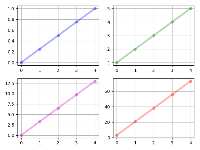
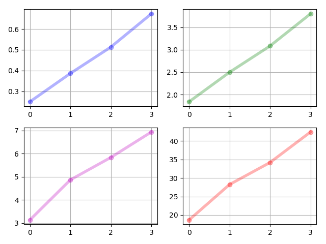
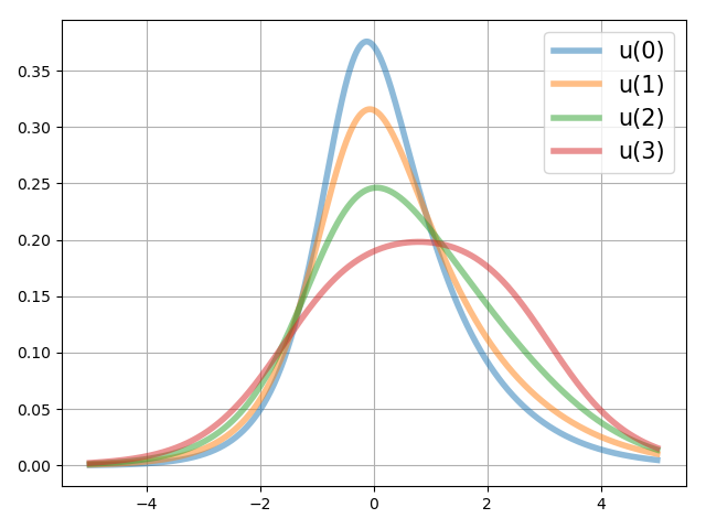
The system parameters are i.i.d. samples drawn from the uniform distribution . The states of the moment system, i.e., for are given in Figure 1. The controls of the moment system, i.e., for are given in Figure 2. We note that by our proposed algorithm, , which makes it feasible for us to realize the controls. The realized control inputs are given in Figure 3. The transition of the control inputs is smooth, which is satisfactory.
In Example 2, we simulate a steering problem in three steps where the initial density function is a Gaussian and the terminal density function is a mixture of generalized logistic distributions. The initial one is chosen as
and the terminal one is specified as
| (28) |
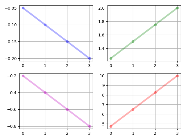
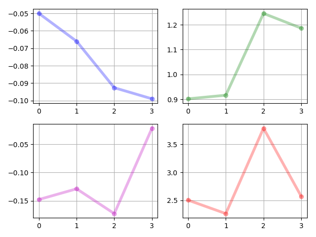
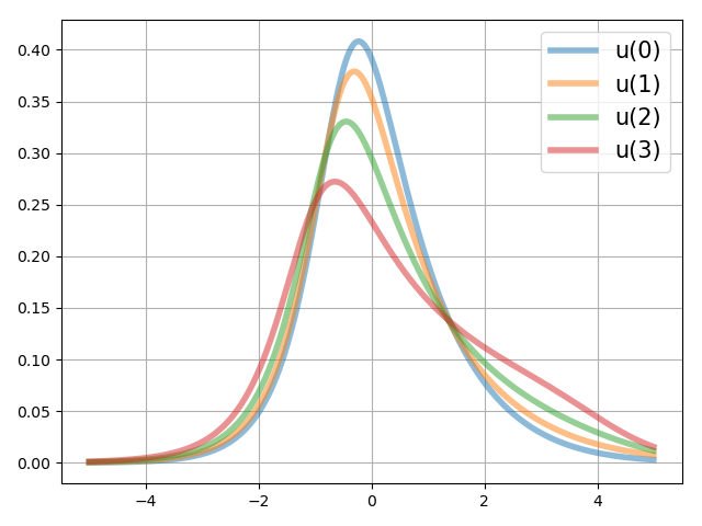
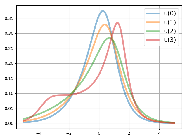
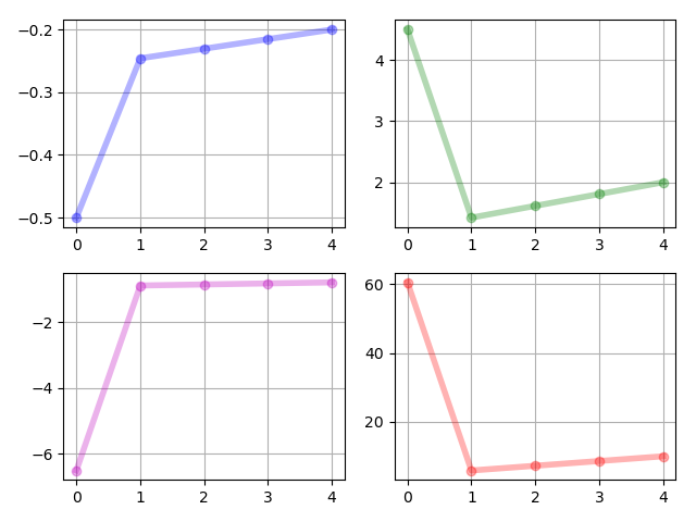
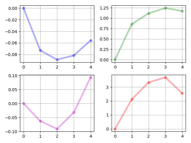
The system parameters are i.i.d. samples drawn from the uniform distribution . The states of the moment system, i.e., for are given in Figure 4. The controls of the moment system, i.e., for are given in Figure 5. The realized controls in Figure 6 also show that the transition of the control inputs is smooth, even the specified terminal density is complicated.
In Example 3, we will simulate a steering problem in four steps which has not been treated in the previous papers. The initial density is chosen as a Gaussian distribution
However the terminal density function is specified as a multi-modal density which is a mixture of two Laplacians
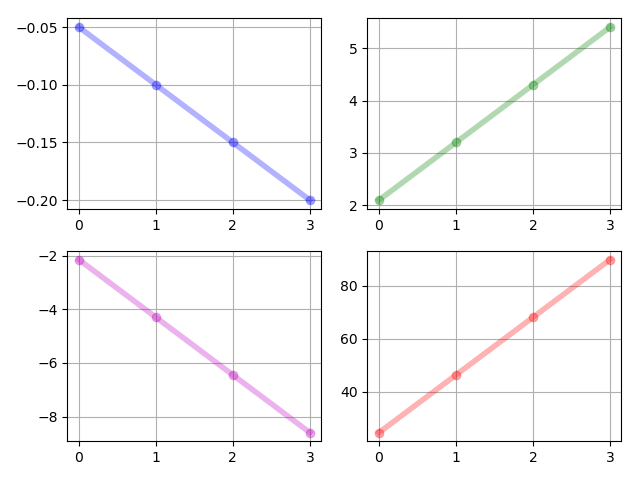
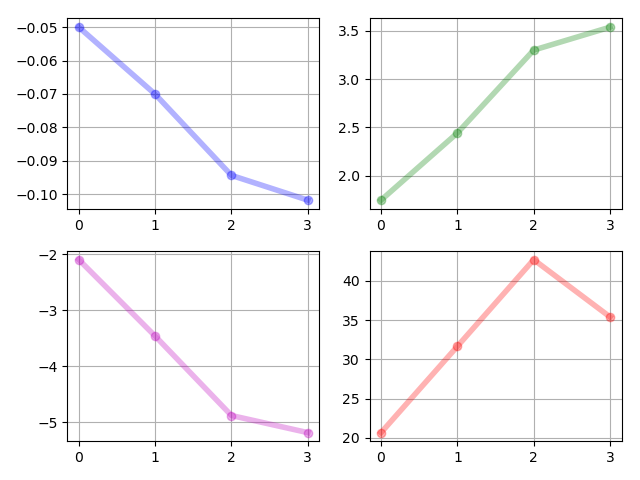
The system parameters are i.i.d. samples drawn from the uniform distribution . The results are given in Figure 7, 8 and 9. In this example, the two modes are not close to each other as in Example 2. However the realized control inputs are still smooth, which validates the performance of our algorithm in steering a group to separate groups relatively far from each other.
4.2 Constrained density steering of a vast group of agents
In some scenarios, there are boundary conditions on the control inputs. A common constraint is that they are bounded by a compact interval on . With our proposed algorithm, we are able to treat the density steering problem with bounded control inputs.
In Example 4, we will simulate a problem which is sort of problematic however important in real practice. The initial and the terminal densities are both chosen as a mixture of two Gaussian densities, which are
and
The density steering is performed in five steps. The control inputs are bounded on the interval . The system parameters are i.i.d. samples drawn from the uniform distribution .
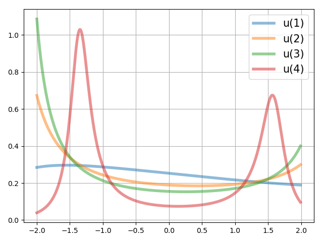
The results are given in Figure 10, 11 and 12. We note that at time step , . Then by the proposed algorithm, we don’t apply control inputs to the agents, which is shown in Figure 11. At time step , we have . Hence we start applying controls starting from this step. It takes three steps for us to steer the density to the specified one.
The goal of the steering in this problem is to steer two distinct groups of agents to two specified terminal groups. The boundary of control inputs and the multiple modality of both initial and terminal densities make the problem a challenging one. By our proposed algorithm, we give a solution to this problem and the realized control inputs are still smooth, which is a satisfactory performance.
Because of (3), we are not able to obtain an analytic by the proposed Algorithm 1, which makes it infeasible to directly compare between and . However fortunately, our proposed algorithm by using the moments is able to treat the occupation measure steering problem. The analytic function at each time step is realized as control inputs of each agent . We can therefore obtain a terminal occupation measure to compare to the specified one. In the following part of this section, we simulate the occupation measure steering examples.
4.3 Occupation measure steering of a vast group of agents
We simulate examples on occupation measure steering in this part of section. In Example 5, we steer agents to a specified occupation measure. The initial states of each agent is drawn i.i.d. from the Gaussian distribution (26). The specified terminal occupation measure consists of i.i.d. samples drawn from the terminal distribution (27). The system parameter are i.i.d. samples drawn from the uniform distribution .
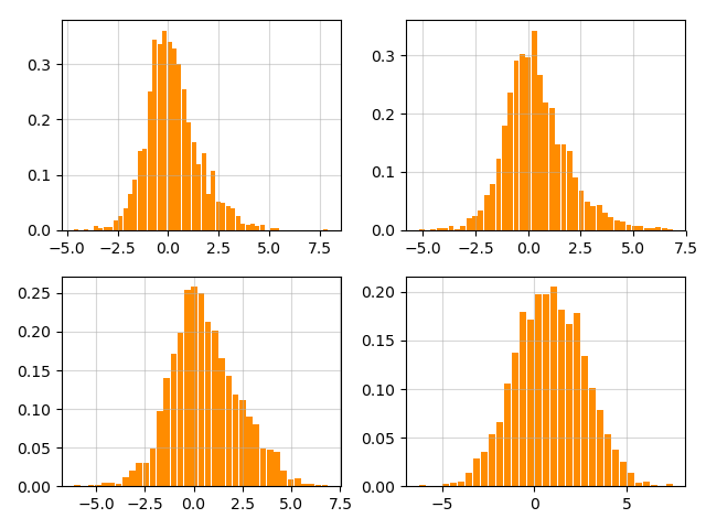
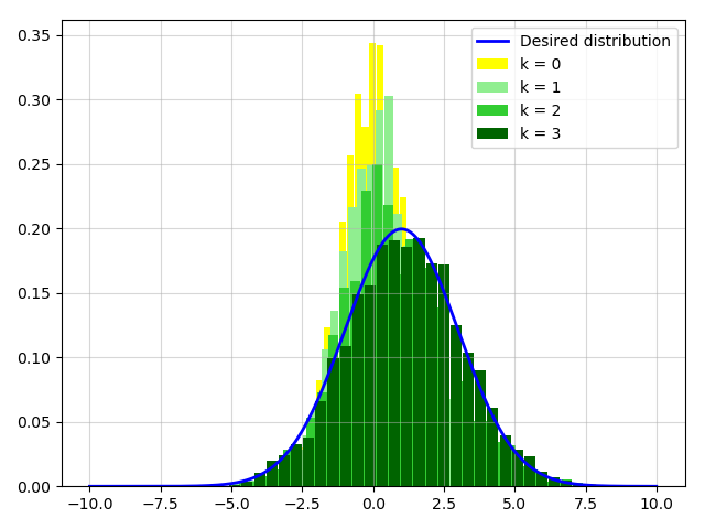
Figure 13 displays histograms of at time step for each agent . These histograms consist of i.i.d samples drawn from the realizations of shown in Figure 3. Additionally, Figure 14 illustrates the histograms of the occupation measure for the states of the agents at time steps . The power moments of order to for the terminal occupation measure, obtained using our proposed algorithm, are respectively. Notably, these values are close to the desired terminal distribution, with power moments of order to being respectively. This outcome validates the effectiveness of our algorithm in steering the occupation measure.
In Example 6, we steer agents to a specified occupation measure. The initial states of each agent is drawn i.i.d. from the Gaussian distribution (26). The specified terminal occupation measure consists of i.i.d. samples drawn from the terminal distribution (28), of which the density is a mixture of two Gaussian densities. The system parameter are i.i.d. samples drawn from the uniform distribution .
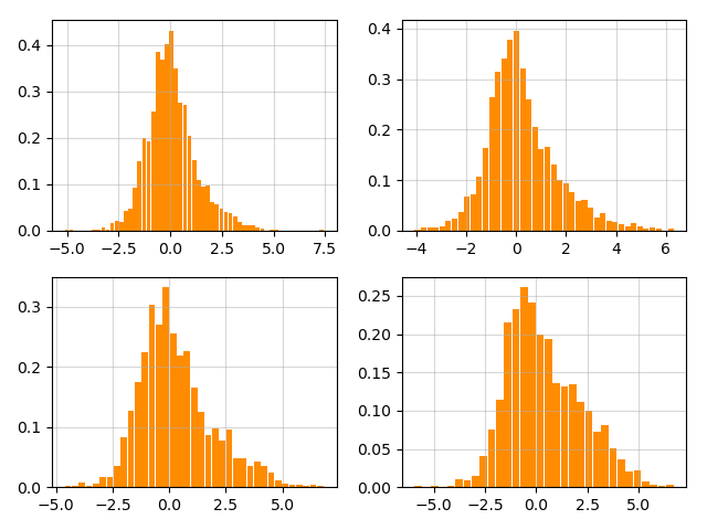
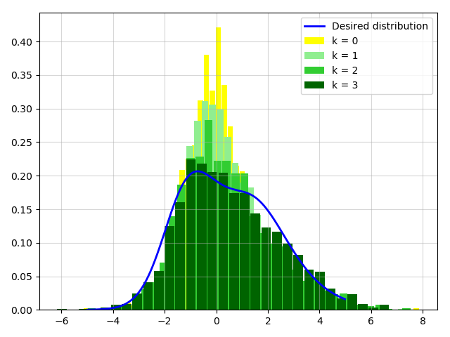
The histograms of at time step for each agent are given in Figure 15. They are i.i.d samples drawn from the realizations of in Figure 6. Figure 16 gives the histograms of the occupation measure of the states of the agents at . We note that the power moments of order to of (28) are respectively. The power moments of order to of the terminal occupation measure by our proposed algorithm are respectively, which are quite close to the specified ones. This example validates the ability of the proposed scheme in treating distribution steering problems with complicated distributions.
5 Concluding remarks
In this paper, we propose to use moments for the problem of steering a vast group of agents. The vast group of agents are characterized as probability density functions and occupation measures. We first treat the density steering problem. Without assuming the initial and terminal density to fall within specific function classes, the original problem is infinite-dimensional and intractable. As to treat this problem, we propose a moment system representation of the original system, and reduce the original problem to the control of the moment system. Different from the conventional control problems, the elements of the control inputs are in the system matrix, and we have to ensure the Hankel matrix of the control inputs at each time step to be positive definite. Since it is not treatable by the existing control schemes including the commonly used optimal control, we propose an empirical control scheme to treat this problem. By doing this, it is feasible for us to realize the control inputs for the original system. The previous results were presented at IFAC World Congress 2023 [28]. In this paper, we consider more fundamental issues of the group steering problems and propose algorithms for real-world group steering problems. We propose that with the number of moment terms used approaching infinity, the terminal distribution obtained by the proposed scheme is almost everywhere equal to the desired one. We also propose an error upper bound of the terminal density by using our proposed algorithm, in the sense of the total variation distance. Our algorithm of steering an arbitrary initial distribution to another arbitrary one in limited steps for the discrete-time first-order ODE systems, without assuming their function classes, is the first one in the literature. Based on the proposed density-steering algorithm, we put forward an algorithm steering an arbitrary occupation measure representing the vast group of agents to another arbitrary one. We use acceptance-rejection sampling to draw i.i.d. samples from the realized control inputs and assign them to each agents. By doing this, the control inputs are independent of the current states of each agent.
This paper treats the group steering problem of the first-order time-variant linear system. However, the problem is much more complicated for multi-order and multivariate systems. For first-order systems, the control inputs ’s are one-dimensional density functions. Hence the positive definiteness of the Hankel matrix of each is the necessary and sufficient condition of the existence of [22]. However for multi-dimensional densities, it is no longer valid. To derive control inputs ’s for the moment system then to realize them will be a challenging problem. Results in subjects e.g. mathematical moment problem and real algebraic geometry shall be used to treat the group steering problem for those systems.
References
- [1] Efstathios Bakolas and Alexandros Tsolovikos. Greedy finite-horizon covariance steering for discrete-time stochastic nonlinear systems based on the unscented transform. In 2020 American Control Conference (ACC), pages 3595–3600. IEEE, 2020.
- [2] Isin M Balci and Efstathios Bakolas. Covariance steering of discrete-time stochastic linear systems based on wasserstein distance terminal cost. IEEE Control Systems Letters, 5(6):2000–2005, 2020.
- [3] Shiba Biswal, Karthik Elamvazhuthi, and Spring Berman. Stabilization of nonlinear discrete-time systems to target measures using stochastic feedback laws. IEEE Transactions on Automatic Control, 66(5):1957–1972, 2020.
- [4] Shiba Biswal, Karthik Elamvazhuthi, and Spring Berman. Decentralized control of multi-agent systems using local density feedback. IEEE Transactions on Automatic Control, 2021.
- [5] Paolo Brandimarte. Handbook in Monte Carlo simulation: applications in financial engineering, risk management, and economics. John Wiley & Sons, 2014.
- [6] Roger W Brockett. Optimal control of the liouville equation. AMS IP Studies in Advanced Mathematics, 39:23, 2007.
- [7] Christopher I Byrnes and Anders Lindquist. A convex optimization approach to generalized moment problems. In Control and modeling of complex systems, pages 3–21. Springer, 2003.
- [8] Kenneth F Caluya and Abhishek Halder. Reflected schrödinger bridge: Density control with path constraints. In 2021 American Control Conference (ACC), pages 1137–1142. IEEE, 2021.
- [9] Yongxin Chen, Tryphon T Georgiou, and Michele Pavon. Optimal steering of a linear stochastic system to a final probability distribution, part i. IEEE Transactions on Automatic Control, 61(5):1158–1169, 2015.
- [10] Yongxin Chen, Tryphon T Georgiou, and Michele Pavon. Optimal steering of a linear stochastic system to a final probability distribution, part ii. IEEE Transactions on Automatic Control, 61(5):1170–1180, 2015.
- [11] Yongxin Chen, Tryphon T Georgiou, and Michele Pavon. Optimal steering of a linear stochastic system to a final probability distribution—part iii. IEEE Transactions on Automatic Control, 63(9):3112–3118, 2018.
- [12] Kai Lai Chung. A course in probability theory. Academic press, 2001.
- [13] Karthik Elamvazhuthi and Spring Berman. Density stabilization strategies for nonholonomic agents on compact manifolds. IEEE Transactions on Automatic Control, 2023.
- [14] Tryphon T Georgiou and Anders Lindquist. Kullback-leibler approximation of spectral density functions. IEEE Transactions on Information Theory, 49(11):2910–2917, 2003.
- [15] Jagat Narain Kapur and Hiremaglur K Kesavan. Entropy optimization principles and their applications. In Entropy and energy dissipation in water resources, pages 3–20. Springer, 1992.
- [16] S. Kullback. Correction to a lower bound for discrimination information in terms of variation. IEEE Transactions on Information Theory, 16(5):652–652, 1970.
- [17] Fengjiao Liu and Panagiotis Tsiotras. Optimal covariance steering for continuous-time linear stochastic systems with martingale additive noise. IEEE Transactions on Automatic Control, 2023.
- [18] Kazuhide Okamoto, Maxim Goldshtein, and Panagiotis Tsiotras. Optimal covariance control for stochastic systems under chance constraints. IEEE Control Systems Letters, 2(2):266–271, 2018.
- [19] Kazuhide Okamoto and Panagiotis Tsiotras. Optimal stochastic vehicle path planning using covariance steering. IEEE Robotics and Automation Letters, 4(3):2276–2281, 2019.
- [20] Joshua Pilipovsky and Panagiotis Tsiotras. Covariance steering with optimal risk allocation. IEEE Transactions on Aerospace and Electronic Systems, 57(6):3719–3733, 2021.
- [21] Augustinos D Saravanos, Isin M Balci, Efstathios Bakolas, and Evangelos A Theodorou. Distributed model predictive covariance steering. arXiv preprint arXiv:2212.00398, 2022.
- [22] Konrad Schmüdgen. The moment problem, volume 14. Springer, 2017.
- [23] Claude Elwood Shannon. A mathematical theory of communication. The Bell system technical journal, 27(3):379–423, 1948.
- [24] Carlo Sinigaglia, Andrea Manzoni, Francesco Braghin, and Spring Berman. Robust optimal density control of robotic swarms. arXiv preprint arXiv:2205.12592, 2022.
- [25] Vignesh Sivaramakrishnan, Joshua Pilipovsky, Meeko Oishi, and Panagiotis Tsiotras. Distribution steering for discrete-time linear systems with general disturbances using characteristic functions. In 2022 American Control Conference (ACC), pages 4183–4190. IEEE, 2022.
- [26] Aldo Tagliani. Maximum entropy solutions and moment problem in unbounded domains. Applied mathematics letters, 16(4):519–524, 2003.
- [27] Aldo Tagliani. A note on proximity of distributions in terms of coinciding moments. Applied Mathematics and Computation, 145(2-3):195–203, 2003.
- [28] Guangyu Wu and Anders Lindquist. Density steering by power moments. IFAC-PapersOnLine, 56(2):3423–3428, 2023.
- [29] Guangyu Wu and Anders Lindquist. Non-Gaussian Bayesian filtering by density parametrization using power moments. Automatica, 153:111061, 2023.
- [30] Silun Zhang, Axel Ringh, Xiaoming Hu, and Johan Karlsson. Modeling collective behaviors: A moment-based approach. IEEE Transactions on Automatic Control, 66(1):33–48, 2020.
- [31] Dongliang Zheng, Jack Ridderhof, Panagiotis Tsiotras, and Ali-akbar Agha-mohammadi. Belief space planning: A covariance steering approach. In 2022 International Conference on Robotics and Automation (ICRA), pages 11051–11057. IEEE, 2022.
- [32] Albert Nikolaevič Širâev, Ralph Philip Boas, and Dmitrij Mihajlovič Čibisov. Probability-1. Springer, 2016.
![[Uncaptioned image]](https://cdn.awesomepapers.org/papers/ca0ff4c4-f0ea-4381-a5d2-11432ab7f424/author1.jpg)
Guangyu Wu received the B.E. degree from Northwestern Polytechnical University, Xi’an, China, in 2013, and two M.S. degrees, one in control science and engineering from Shanghai Jiao Tong University, Shanghai, China, in 2016, and the other in electrical engineering from the University of Notre Dame, South Bend, USA, in 2018.
He is currently pursuing the Ph.D. degree at Shanghai Jiao Tong University. His research interests are the moment problem and its applications to stochastic filtering, stochastic control and statistics.
![[Uncaptioned image]](https://cdn.awesomepapers.org/papers/ca0ff4c4-f0ea-4381-a5d2-11432ab7f424/author2.jpg)
Anders Lindquist received the Ph.D. degree in optimization and systems theory from the Royal Institute of Technology, Stockholm, Sweden, in 1972, and an honorary doctorate (Doctor Scientiarum Honoris Causa) from Technion (Israel Institute of Technology) in 2010.
He is currently a Zhiyuan Chair Professor at Shanghai Jiao Tong University, China, and Professor Emeritus at the Royal Institute of Technology (KTH), Stockholm, Sweden. Before that he had a full academic career in the United States, after which he was appointed to the Chair of Optimization and Systems at KTH. Dr. Lindquist is a Member of the Royal Swedish Academy of Engineering Sciences, a Foreign Member of the Chinese Academy of Sciences, a Foreign Member of the Russian Academy of Natural Sciences, a Member of Academia Europaea (Academy of Europe), an Honorary Member the Hungarian Operations Research Society, a Life Fellow of IEEE, a Fellow of SIAM, and a Fellow of IFAC. He received the 2003 George S. Axelby Outstanding Paper Award, the 2009 Reid Prize in Mathematics from SIAM, and the 2020 IEEE Control Systems Award, the IEEE field award in Systems and Control.