Gyrokinetic and kinetic particle-in-cell simulations of guide-field reconnection. I. Macroscopic effects of the electron flows
Abstract
In this work, we compare gyrokinetic (GK) and fully kinetic Particle-in-Cell (PIC) simulations of magnetic reconnection in the limit of strong guide field.
In particular, we analyze the limits of applicability of the GK plasma model compared to a fully kinetic description of force free current sheets for finite guide fields ().
Here we report the first part of an extended comparison, focusing on the macroscopic effects of the electron flows.
For a low beta plasma (), it is shown that both plasma models develop magnetic reconnection with similar features in the secondary magnetic islands if a sufficiently high guide field () is imposed in the kinetic PIC simulations. Outside of these regions, in the separatrices close to the X points, the convergence between both plasma descriptions is less restrictive ().
Kinetic PIC simulations using guide fields reveal secondary magnetic islands with a core magnetic field and less energetic flows inside of them in comparison to the GK or kinetic PIC runs with stronger guide fields.
We find that these processes are mostly due to an initial shear flow absent in the GK initialization and negligible in the kinetic PIC high guide field regime, in addition to fast outflows on the order of the ion thermal speed that violate the GK ordering.
Since secondary magnetic islands appear after the reconnection peak time, a kinetic PIC/GK comparison is more accurate in the linear phase of magnetic reconnection.
For a high beta plasma () where reconnection rates and fluctuations levels are reduced, similar processes happen in the secondary magnetic islands in the fully kinetic description, but requiring much lower guide fields ().
Copyright (2015) American Institute of Physics. This article may be downloaded for personal use only. Any other use requires prior permission of the author and the American Institute of Physics.
The following article appeared in P. A. Muñoz, D. Told, P. Kilian, J. Büchner and F. Jenko, Physics of Plasmas 22, 082110 (2015), and may be found at
http://dx.doi.org/10.1063/1.4928381
I Introduction
Magnetic reconnection is a fundamental process in plasma physics that converts magnetic field energy efficiently into plasma heating, kinetic energy of bulk flows and accelerated particles. It plays a role in a wide range of different environments, from fusion devices, planetary magnetospheres, and stellar coronae to extragalactic accretion disks.Büchner (2007); Zweibel and Yamada (2009); Yamada, Kulsrud, and Ji (2010)
Originally, magnetic reconnection was modeled with antiparallel magnetic fields in a plane sustained by a current sheet (CS). But that configuration is not common in nature, since the presence of an out-of-plane magnetic field is ubiquitous in both space and laboratory plasmas, such as in the solar corona and fusion devices, respectively. However, the properties of reconnection in the presence of a guide field () are still nowadays much less understood.Treumann and Baumjohann (2013) Thus, the study of stability of these CS with shear magnetic fields is of paramount importance to understand the conversion of magnetic energy in these environments.
In order to capture the kinetic effects in magnetic reconnection, fully kinetic particle-in-cell (PIC) codes have become one of the preferred tools since some time ago, with the increasing availability of computational resources.Büchner, Dum, and Scholer (2003) These codes allow the simulation of magnetic reconnection in fully collisionless Vlasov plasmas. However, these fully kinetic PIC simulations (for brevity, from now on these ones will be simply referred to as “PIC simulations”) can be computationally very demanding due to stability reasons and the requirement of keeping numerical noise as low as possible. One approach to solve this problem is using gyrokinetic (GK) theory, an approximation to a Vlasov plasma (see Ref. Frieman and Chen, 1982 or Refs. Brizard and Hahm, 2007; Howes et al., 2006; Schekochihin et al., 2009 for more recent reviews). In this plasma model, the idea is to decouple the fast gyrophase dependence from the dynamics, considering the motion of charged rings, thus reducing the phase space from six to five dimensions and removing dynamics on very small space-time scales. The gyrokinetic approach is suitable in strongly magnetized plasmas (equivalent to the limit of very large magnetic guide fields in magnetic reconnection). More precisely, the ion gyroradius has to be much smaller than the typical length scale of the background: , where is the GK ordering parameter. In contrast, it is important to note that the typical length scale of variation of the perpendicular perturbations, , can be comparable to the ion gyroradius: . The ordering implies the restriction of the GK approach to phenomena with frequencies lower than the ion cyclotron one: , where is a typical frequency in the system. The fluctuations in the distribution function and electromagnetic fields, with respect to their equilibrium values, are also of order . And finally, these fluctuations are assumed to have much larger scales along the magnetic field direction than across it: , where and are the wavevectors along and across the magnetic field, respectively. An important consequence of this assumption is that the perpendicular bulk speed is mostly dominated by drifts, which have to be smaller than the ion thermal speed according to . This fact will be a source of differences between the GK and kinetic simulations that do not have such a restriction.
Simulations of magnetic reconnection with codes based in the GK theory have shown to drastically reduce the computation time, which allows the use of more realistic numerical parameters (e.g.: mass ratio), and at the same time, the possibility to capture many of the desired kinetic effects, such as finite ion Larmor radius ones.Wan, Chen, and Parker (2005); Rogers et al. (2007); Pueschel et al. (2011, 2014) However, one of the drawbacks of the GK simulations of magnetic reconnection is that the initial setup has to be force free . The often used Harris sheetHarris (1962) initialization is not possible in the standard gyrokinetic theory, since the particles that carry the current are different from the background, and therefore the perturbed current is of second order in the ordering GK parameter . Nevertheless, a force free initialization is a good approximation to the exact kinetic equilibrium in low beta plasmas with strong guide field.
Due to the previous reasons, it is of fundamental importance to establish the key properties of magnetic reconnection that can be properly modeled with a gyrokinetic code, instead of running computationally expensive fully kinetic PIC simulations. In this context, the first direct comparison between PIC and GK simulations of magnetic reconnection in the large guide field limit was performed just recently in Ref. TenBarge et al., 2014. They found that many reconnection related fluctuating quantities (such as the thermal/magnetic pressures) obtained for different PIC guide field runs have the same value after they are scaled to . And this value is equal to the result given by the GK simulations after a proper choice of the parameter. This is valid under the assumption of a constant total plasma (to be defined in Sec. II) among different PIC guide field runs. The result is in agreement with the predictions of a two fluid analysis of Ref. Rogers, Denton, and Drake, 2003. In addition, Ref. TenBarge et al., 2014 showed that the morphology of the out-of-plane current density exhibits a good convergence between the PIC simulations with sufficiently high guide field and the gyrokinetic runs. They also noticed that low plasmas require higher PIC guide fields to reach convergence towards the GK results, in comparison to high plasmas.
However, the previous benchmark study in Ref. TenBarge et al., 2014 did not discuss some limitations in the GK approach, that might make a comparison with a fully kinetic description of magnetic reconnection not reliable in some parameter regimes. In this context, our purpose is investigating the physical origin of the differences between these plasma models in the realistic regime of finite PIC guide fields (since PIC cannot use arbitrarily large values of guide field, where results should match). Thus, we aim to establish the limits of applicability of the GK compared to PIC simulations of magnetic reconnection. Some of the differences come from the special way in which the GK plasma model enforces the force balance in the perpendicular direction to the magnetic field to order . Indeed, from the perpendicular GK Ampère’s law, it can be provenRoach et al. (2005); Schekochihin et al. (2009); Abel et al. (2013)
| (1) |
Here, the quantities denoted as are of order . is the (total) perturbed perpendicular pressure tensor and the perturbed parallel magnetic field. This expression is satisfied exactly to order , being formally equivalent to the pressure equilibrium condition as given by the two fluid model in the strong guide field limit (to be discussed in Eq. (7)). The only difference is that can possibly include off-diagonal elements representing finite Larmor radius effects in the GK model, while in the two-fluid model the thermal pressure is only a scalar quantity. Note that even though the magnetic pressure is much larger than the thermal pressure in this force free scenario, their gradients or fluctuations can still be comparable, and that is why such pressure equilibrium still exists even in the strong guide field limit as assumed in the GK approach. On the other hand, there is no such restriction in the PIC approach, but it converges towards it as the guide field increases.
The physical consequence of the previous fact is that the agreement between both approaches breaks down mostly when secondary magnetic islands, with strongly unbalanced magnetic pressures, appear in the PIC simulations using a (relatively) low guide field. Although they also appear in the PIC high guide field regime or the GK simulations, these secondary magnetic islands have different features as a result of an initial shear flow present in the PIC force free initialization. These secondary magnetic islands are structures that appear as a result of the tearing mode, with a different (smaller) wavelength than the one imposed by the large scale initial perturbation. They start at electron length scales, growing up to ion scales. In this sense, our definition does not exactly match with some previous studies,Chen, Daughton, and Bhattacharjee (2012); Zhou, Deng, and Huang (2012); Huang et al. (2014) which limit secondary islands to those ones with electron length scales. Other works have stated that secondary islands have opposite out-of-plane current density to those of the primary islands.Huang et al. (2013) Again, the structures in our simulations do not match these features.
We expect the formation of these structures in our setup, since it is known that guide field reconnection produce a “burstier” reconnection, forming more secondary magnetic islands than an antiparallel configuration.Drake et al. (2006) Many previous works have analyzed these structures with several levels of details, in particular in the context of extended current layers, since they can modulate temporally the reconnection rates (see Ref. Daughton et al., 2011 and references therein). For example, the authors of Ref. Karimabadi et al., 1999 reported a core magnetic field inside of secondary magnetic islands by means of hybrid simulations of Harris sheets with a weak magnetic guide field. It was attributed to a nonlinear amplification mechanism between the guide field and the out-of-plane magnetic field generated by Hall currents. Later, Zhou et al. (2014) analyzed the same phenomenon during the coalescence of secondary magnetic islands, with 2D PIC simulations for a similar setup. In our case, we will show that a similar consequence takes place but as a result of a shear flow initialization in the PIC low guide field regime.
Shear flows have been analyzed exhaustively for their importance in the development of magnetic reconnection. It is known that reconnection rates decrease with faster shear flows parallel to the reconnected magnetic field, according to the scaling law derived in Ref. Cassak, 2011 under a Hall-MHD model without guide field (basically, due to less efficient outflows from the X point). A kinetic approach and PIC simulations have confirmed this prediction, but have also shown that tearing mode (associated with the formation of magnetic islands) is never completely stabilized for thin CS, even with super-Alfvénic flows.Roytershteyn and Daughton (2008) A two-fluid analytical studyHosseinpour and Mohammadi (2013) of collisionless tearing mode driven by electron inertia showed that a shear flow, under certain conditions, can generate a symmetric out-of-plane magnetic field. Shear flows are also closely related with the Kelvin-Helmholtz instability. Our PIC runs in the low guide field regime do not exhibit outflows with sufficient speed to drive the kinetic version of Kelvin-Helmholtz, mostly because they scale as the Alfvén speed which is known to be a threshold for this instability.Wang, Pritchett, and Ashour-Abdalla (1992) It is also important to mention the work by Fermo, Drake, and Swisdak (2012) and Liu et al. (2014), which found, by means of 2D PIC simulations, secondary magnetic islands generated by the Kelvin-Helmholtz instability in the reconnection outflow (similar to the finding by Loureiro, Schekochihin, and Uzdensky (2013), but in the framework of reduced MHD). On the other hand, the structures observed in our case appear only close to the main X point. However, the secondary magnetic islands in our PIC/GK simulations share some of the features seen in those previous works. That is why we are going to relate their appearance with the core magnetic field and shear flow, depending on the parameter regimes of our PIC/GK runs.
The remainder of this paper is organized as follows. In Sec. II, we describe the simulation setup used by both GK and PIC codes, as well as the parameter range to be studied. In Sec. III we identified the deviations from the linear scaling on the guide field of some magnetic reconnection quantities, extending the previous comparison work by TenBarge et al. (2014) These differences between PIC and GK simulations, appearing for some parameter regimes and specific spatial and temporal locations, are manifested in both magnetic and thermal pressure fluctuations. In this paper we focus on the first ones, while the deviations with respect to the linear scaling in the thermal pressure fluctuations will be deferred to a follow-up paper. The remarkably high values of magnetic fluctuations in the PIC low guide field regime are due to the generation of a core magnetic field in the secondary magnetic islands. This process is discussed in Sec. IV in the context of two fluid theory and violations of the pressure equilibrium condition. Then, in Sec. V, we analyze the physical mechanism of this core magnetic field as a result of a shear flow due to the force free initialization in the PIC low guide field runs. We briefly discuss the effects of a high plasma on all these processes in Sec. VI. Finally, we summarize our findings in the conclusion, Sec. VII.
II Simulation setup
The results of the 2.5D simulations (no variations allowed in the out-of-plane direction ) to be shown were obtained with the explicit fully kinetic PIC code ACRONYMKilian, Burkart, and Spanier (2012) and the gyrokinetic GENE code.Jenko et al. (2000) For both PIC and gyrokinetic simulations, we used a very similar setup and parameter set to the ones used in Ref. TenBarge et al., 2014. We will repeat here the more important parameters to ensure a future accurate reproducibility of our work. The initial equilibrium is a force free double CS, with halfwidth and magnetic field given by:
| (2) | ||||
| (3) |
with relative guide field strength , where is the (asymptotic) reconnected magnetic field. This corresponds to a total magnetic field of constant magnitude . A change in is obtained by modifying but always keeping constant (note that Ref. TenBarge et al., 2014 keeps constant, but if and so the differences are not significant in this regime). and are the simulation box sizes in the reconnection plane -, respectively. Ions are initially stationary, while the current is carried by drifting electrons with velocity according to , satisfying the Ampère’s law . are the initial constant electron (“e”) and proton (“i”) number densities, respectively. In order to accelerate the reconnection onset, we use a perturbation in and that generates an X/O point at the center of the left/right CS and that can be derived from the vector potential
| (4) |
where is the amplitude of the perturbation. The parameters used in this study are divided in two sets: “low” and “high” beta cases, being summarized in Table 1. All the corresponding quantities are calculated with respect to , i.e.: the ion plasma beta , the electron/ion cyclotron frequency and the electron/ion Larmor radius , with the electron/ion thermal speed . We also have equal temperatures for both species , implying . All the details concerning normalization and the appropriate correspondence between GK and PIC results can be found in the Appendix A.
| Case | |||||
|---|---|---|---|---|---|
| Low beta | 0.01 | 0.8 | 0.125 | 2 | 40 |
| High beta | 1.0 | 4.0 | 0.25 | 1 | 20 |
Now, let us specify some numerical parameters. For all cases we use a reduced mass ratio . Both codes use double periodic boundary conditions ( and directions). For the PIC runs, we use a grid size such as cells in the low beta case (with ), while for the high beta case is cells (with ). The time step is chosen to be in the low/high beta case, respectively, to fulfill the Courant-Friedrichs-Lewy (CFL) condition (for light waves) with . Thousand particles per cell are used in both cases for each species. A second order interpolation scheme, also known as TSC shape function (Triangular Shaped Cloud) was used to reduce numerical noise without having to increase significantly the macroparticle number. Finally, no current smoothing was used. For the GK runs, the spatial grid is for both cases, while the parallel/perpendicular velocity grid is chosen to be , , with 3220 points in the space (). is the (adiabatic invariant) magnetic moment. In the GK simulations, the initial noise level and spectrum were chosen to match with the corresponding one in the PIC runs. Then, this noise acts as an additional perturbation on top of the one described in Eq. (4).
Finally, some comments about the computational performance of the runs with our codes under the different parameter regimes of this study can be found in the Appendix C.
III Global evolution and deviations from linear scaling
In this section, we first show the global evolution of the GK/PIC simulations comparing with the results obtained by TenBarge et al. (2014) Then, we explain and quantify the linear scaling on the guide field as predicted by the two fluid model of Ref. Rogers, Denton, and Drake, 2003, in order to identify the deviations from it and the key open problems that will be addressed in this and an upcoming paper.
III.1 Global evolution
With our independent set of codes, the PIC code ACRONYM and the GK code GENE, we obtained similar values for the reconnection rates (see Fig. 1) as the ones reported by the previous comparison work, Ref. TenBarge et al., 2014. First, the normalized reconnection rates have the same value for each high/low case for different guide fields (although they decrease with when measured without normalization, consequence of keeping constant the total plasma ). The constancy of normalized reconnection rates in the strong guide field limit agrees with some previous studies, even when the total plasma changesLiu et al. (2014) (and correspondingly it was expected to have different reconnection regimes). Note that is not valid for Harris CS in the very low guide field regime, where it is known that the normalized reconnection rates are reduced with increasing (see, e.g., Refs. Pritchett, 2001; Pritchett and Coroniti, 2004; Ricci et al., 2004), as a result of the enhanced incompressibility of the plasma.
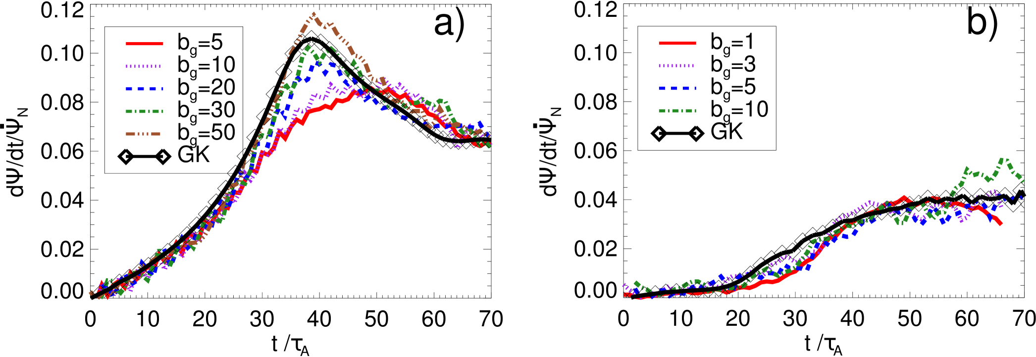
Second, we also found smaller reconnection rates in the high beta case compared to the low beta one, in agreement with previous studies of gyrokinetic simulations of magnetic reconnection.Numata and Loureiro (2014, 2015) However, we can notice in Fig. 1 that the reconnection values for both low and high plasma cases are still a substantial fraction of . Therefore, fast magnetic reconnection takes place in both cases, even though the low beta runs are in a regime where there should be not dispersive waves that may explain these rates, according to the two fluid analysis in Ref. Rogers et al., 2001 (see also Ref. Ricci et al., 2004). This contradiction was already addressed in Ref. TenBarge et al., 2014 and also other recent works.Liu et al. (2014); Stanier et al. (2015); Cassak et al. (2015) Although there is no a full definitive answer to this controversy yet, all these evidences seem to indicate that fast dispersive waves, such as whistler and kinetic Alfvén waves, seem not to play the essential role to explain fast magnetic reconnection in collisionless plasmas. Since the purpose of this paper is different, we are not going to discuss further that issue in this work.
It is worth to mention that some details in the evolution of the system are not exactly the same as in Ref. TenBarge et al., 2014. For instance, in the low beta case (Fig. 1(a)), although the peak in the reconnection rate is reached more or less at the same time, we observed that the CS is more prone to the development of secondary islands than reported there. They start to appear just after the reconnection peak () instead of . Probably, this is due to the different initial noise level in the PIC runs, since it is random and dependent on the specifics of the algorithms implementation. Therefore, the locations and timing of the secondary magnetic islands are expected to be different between the results given by the VPIC (as used in Ref. TenBarge et al., 2014) and ACRONYM codes (and also with the GK code GENE).
All the results and plots to be shown from now on are based in the low beta case. The slightly different conclusions for the high beta case will be briefly analyzed only in Sec. VI.
III.2 Parity/symmetry of magnetic reconnection quantities and linear scaling
As indicated in Ref. TenBarge et al., 2014, based in the two fluid analysis of Ref. Rogers, Denton, and Drake, 2003, the thermal pressure and magnetic field fluctuations should display antisymmetric (odd-parity) structures in the separatrices in the strong guide field regime , assuming small enough fluctuations and asymptotic plasma beta (although a later studyHosseinpour and Mohammadi (2013) showed that this assumption is not necessary for the appearance of an odd-parity magnetic field structure). In addition, both quantities should scale inversely with the guide field in the following way (see Eqs. (17) and (19) of Ref. Rogers, Denton, and Drake, 2003):
| (5) | ||||
| (6) |
where is the typical length scale of variation of these quantities across the CS, away enough from the X points. The fluctuations are calculated by subtracting the (initial) equilibrium quantities (for ) and (for brevity, we omit the subscript in the thermal pressure). Note that in deriving the previous expressions, the pressure equilibrium condition in the limit of strong guide field has been usedRogers, Denton, and Drake (2003) (also obtained in the framework of reduced MHD), formally equivalent (by assuming a scalar pressure) to the perpendicular force balance of the more general GK equations as given in Eq. (1) (satisfied exactly to order ). This can be written in the following way by combining the previous expressions for and :
| (7) |
Note that Eqs. (5) and (6) predict that the fluctuations and are proportional to providing and constant for different guide fields, which is valid recurring to the estimate of order of magnitude given in Ref. Rogers, Denton, and Drake, 2003. The last assumption requires additional evidence in order to be applied to our simulations, and that is why we proved this claim via the method explained in detail in the Appendix B. Using the suitable normalizations explained in Appendix A, we show the estimates for and in Fig. 2 and Fig. 3, respectively, for a time shortly after the reconnection peak. These and all the other figures from the PIC runs shown in this paper, unless stated otherwise, have been averaged over to reduce the effects of the numerical noise. In addition, the color scheme is scaled between the mean plus 3.5 standard deviations of the plotted quantity, a representative maximum as explained in the discussion of Fig. 5.
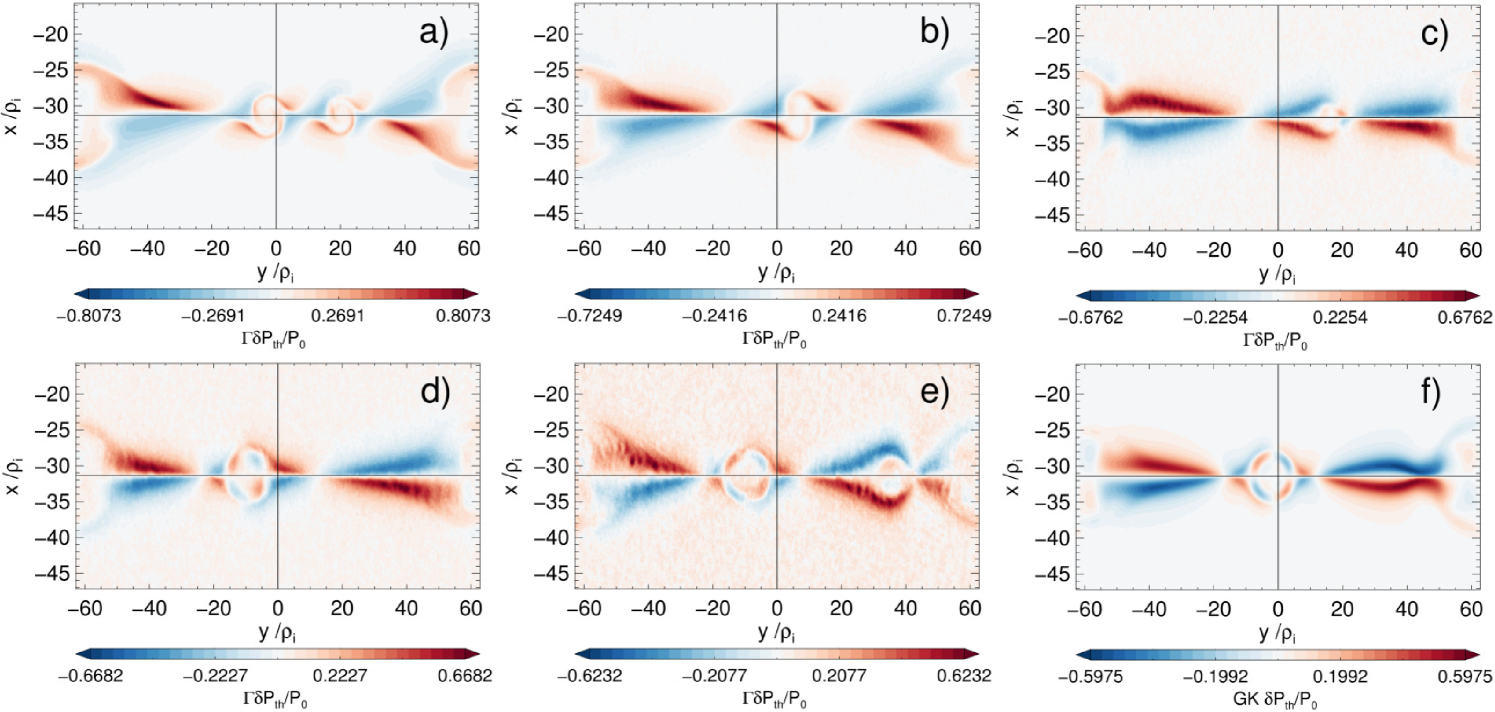
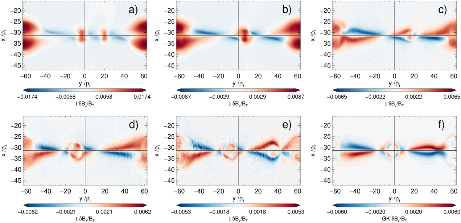
From Figs. 2 and 3 we confirm the result already found in Ref. TenBarge et al., 2014 and predicted by the previously sketched two fluid model:Rogers, Denton, and Drake (2003) the convergence of the PIC results towards the GK ones in the limit of strong guide field, in both odd symmetry and scaling with the guide field. As discussed by these authors, this is valid only in the region close to the separatrices. However, we can immediately notice a fact not discussed in the previous comparison work: not only the symmetry between both separatrices is broken in the low guide field regime, but also the appearance of an additional magnetic field in the secondary magnetic islands not visible in GK or in the limit of strong PIC guide field. This is the main difference and new result to be the focus of the remainder of this work. For brevity, other differences between PIC/GK will be addressed in a follow-up paper.
IV Core magnetic field and pressure equilibrium condition
The core magnetic field in the secondary magnetic islands, as well as in the boundaries, can be understood from several points of view. In this section, we will describe it in the framework of deviations from the two fluid model sketched in Sec. III.2, based on the pressure equilibrium condition.
IV.1 Pressure equilibrium condition in the strong guide field limit in GK/PIC
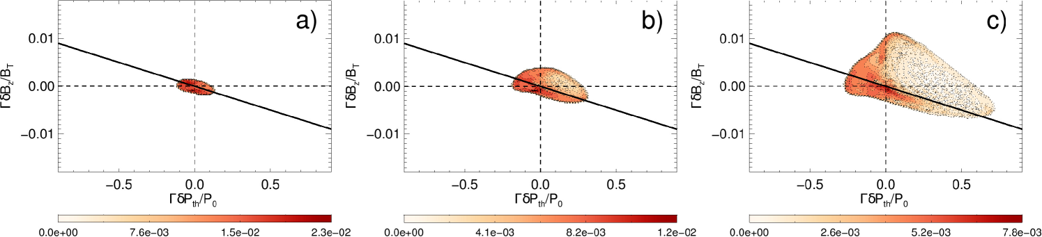
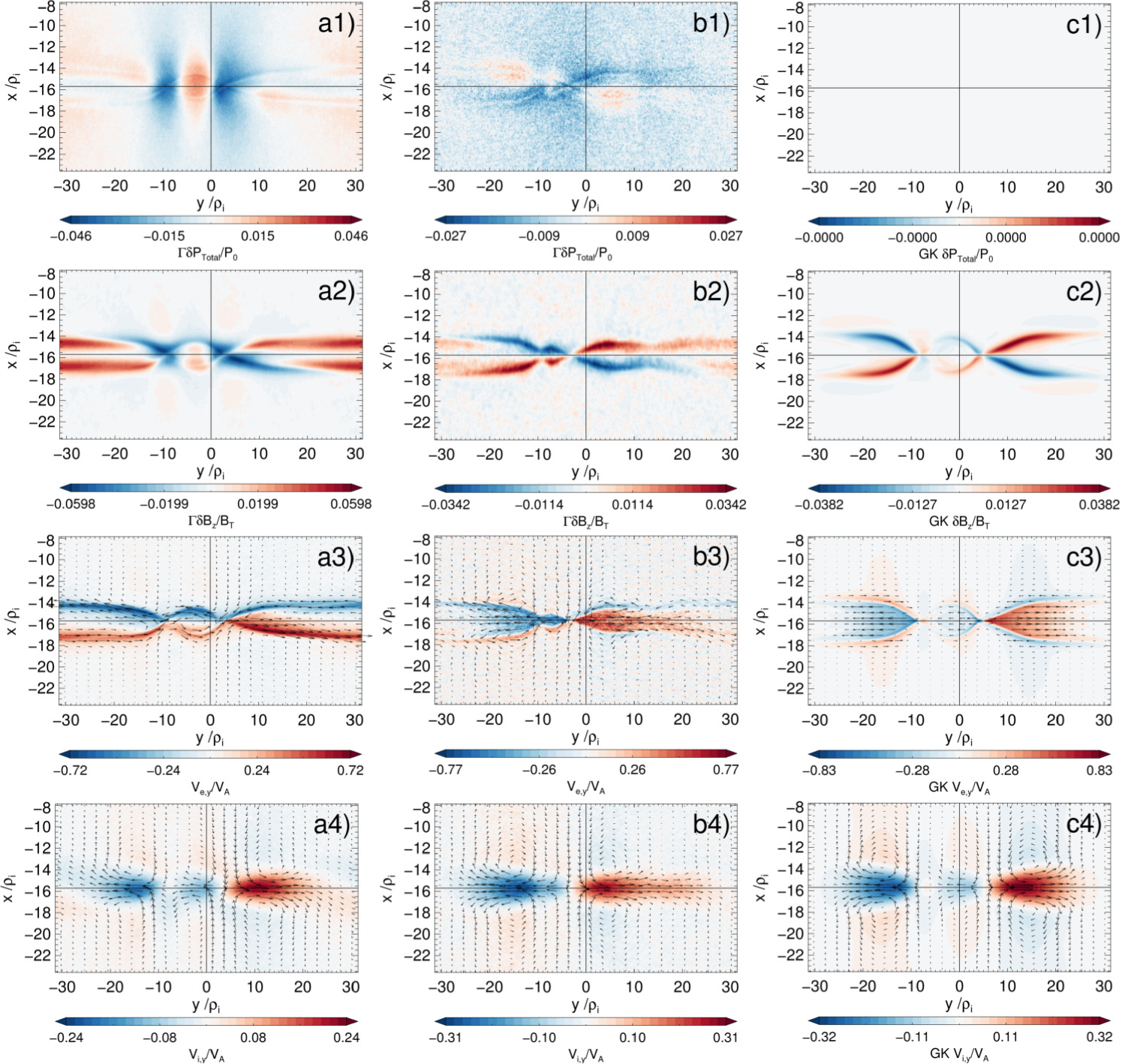
The core magnetic field in the secondary magnetic islands and boundaries is unbalanced, in the sense that the thermal pressure does not decrease at these locations (compare Figs. 2 with 3). This is a violation of the pressure equilibrium condition in the strong guide field limit as given in Eq. (1) or Eq. (7). Since it is satisfied exactly to order in GK, it is built-in in the equations that the GENE code solves, while PIC codes allow large deviations from it for finite guide fields, since they solve the full collisionless Vlasov-Maxwell system of equations. Note, in particular, that Eq. (7) represents a straight line with slope in the plane - . Therefore, a convenient way to display this relation and deviations is by means of a 2D (frequency) histogram of these fluctuating quantities, with results shown in Fig. 4(middle row). These plots were generated by selecting the interesting region close enough to the center of the CS with above of its initial value, indicated in Fig. 4(top row). In order to show the locations of deviations in the pressure equilibrium condition, we also plot in Fig. 4(bottom row) the corresponding fluctuations in the total pressure
| (8) |
with .
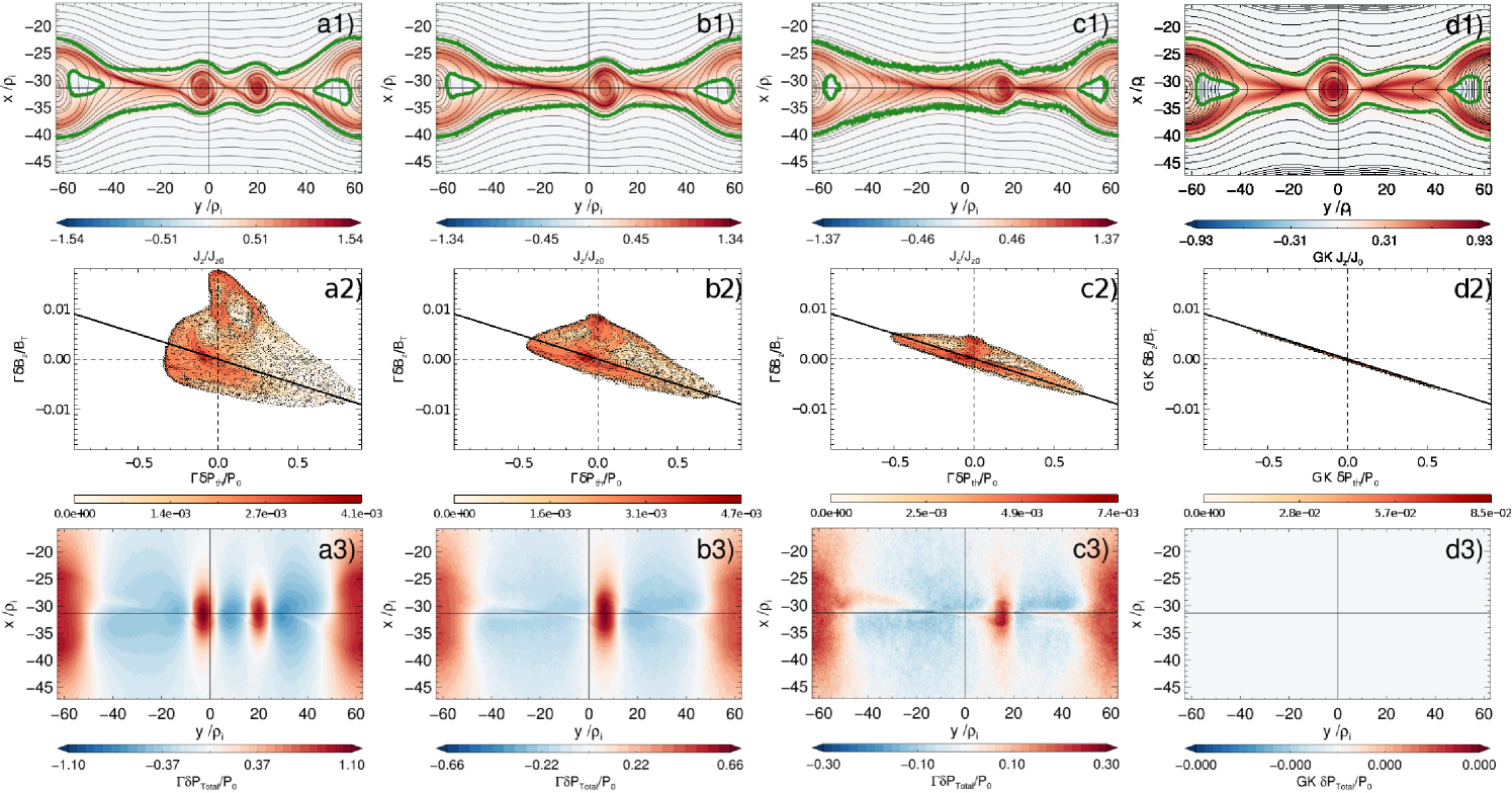
Top row: Contour plots of the out-of-plane current density . Magnetic field lines are shown in black contour lines. The region inside of the green contour satisfies .
Middle row : 2D (frequency) histograms with the correlation between the magnetic and thermal fluctuations and . The diagonal black straight line is the pressure equilibrium condition Eq. (7).
Bottom row: Contour plots for the scaled total pressure . Note that to machine precision in GK (d3).
Fig. 4(middle row) shows that most of the locations in the CS are along the line for the case PIC , with an increasing spread in the lower regime. The corresponding GK results follow very accurately that line. Note a distinctive, pressure unbalanced, “bump” in the region with , being very noticeably for the case PIC . Fig. 4(bottom row) shows that these regions are mostly in the secondary magnetic islands and in the boundaries. This excess of total pressure generates a net force towards the exterior of the magnetic islands, leading to an expansion in reconnection time scales (). increases going to the lower guide field regime, even though this quantity has been linearly scaled to . That is to be expected, since the high fluctuation level in these cases breaks down the small assumption in which Eqs. (5),(6) or (7) (and also Eq. (1)) are based.
Note that the histograms for low show a strongly asymmetric distribution in comparison with GK or PIC high regime (see Fig. 4(middle row)): there are more points located in the right bottom quadrant ( and ) than in the left upper quadrant ( and ). This is an indication of (and an efficient way to quantify) the asymmetry in the separatrices for the PIC low guide field regime (see the respective contour plots Figs. 2 and 3). We will explain the reasons in Sec. V.1.
We can summarize these findings by saying that, although the magnetic field fluctuations predicted by the GK simulations can be comparable to the PIC ones in the low guide field regime ( and ) close to the separatrices, this is not true inside of the secondary magnetic islands or the periodic boundaries, due to the deviation in the pressure equilibrium Eq. (1).
IV.2 Time evolution of magnetic and thermal fluctuations
The purpose of this subsection is to analyze the dynamical evolution of the thermal and magnetic fluctuations, complementing the work by TenBarge et al. (2014). This allow us to determine the physical mechanisms producing the deviations in the pressure equilibrium condition, as well as the asymmetric separatrices in the PIC low guide field regime. We quantify this by means of tracking the “maximum” of and in the entire region shown in Figs. 2 and 3. For the PIC simulations, in order to decrease the effects of the numerical noise, this “maximum” is chosen as equal to the mean plus 3.5 standard deviations. The absolute maximum is not a good choice since is very prone to outlier values. In addition, the initial value of the respective fluctuating quantity is subtracted (note that it is not only the initial value and ), because: (1) a zero offset is required by GK since the fluctuating quantities are initially zero and (2) it mostly measures the numerical PIC noise, being enhanced for higher . The results are shown in Fig. 5.
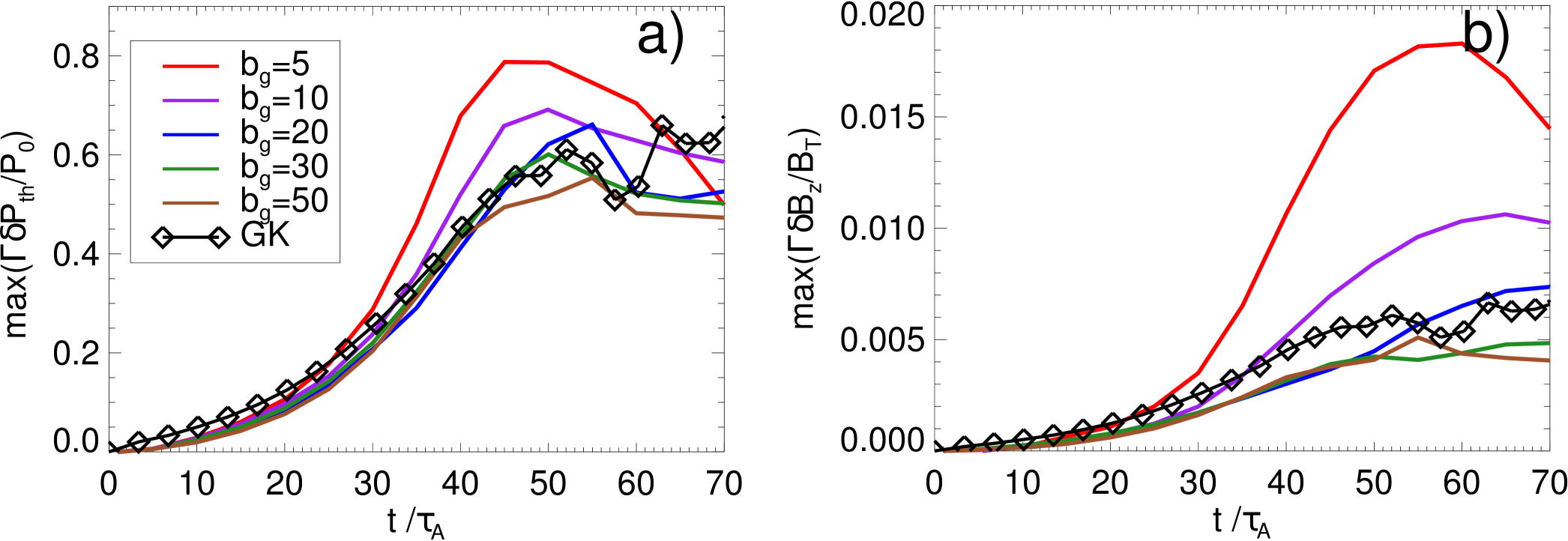
First of all, Fig. 5(a) shows that the maximum of is reached around for all the cases, after the reconnection peak time when also the secondary magnetic islands start to form. reaches maximum values even later. This in an indication of an additional mechanism generating , different from the one produced by the Hall currents due to the reconnection process itself (close to the X point, in the separatrices), and deeply in the non-linear phase. This is also the justification for showing the contour plots at a time in most of the figures of this paper.
By means of the results shown in Figs. 5(a) and 5(b), we also confirm (complementing the work of Ref. TenBarge et al., 2014) the convergence of the time evolution of both PIC and toward the GK curves in the strong guide field limit . As can be expected, the GK values follow a similar trend as the strongest PIC guide field (). However, there are important deviations in some curves, noticeable earlier for smaller . For example, the PIC run shows deviations from the GK curve of already in , while only after . Note that the deviations in are smaller than those of . The (interesting) physical reasons of the differences for will be addressed in a follow-up paper. Here we explain and analyze with more detail the differences in shown in Fig. 5(b).
Although useful, Fig. 5 cannot provide us with information about the relation of these maxima with the pressure equilibrium condition Eq. (7). For this purpose, in Fig. 6 we show the 2D histograms relating these fluctuations in the plane for three characteristic times during the evolution of the case PIC .
The asymmetry along the pressure equilibrium line located in the right bottom part ( with ) starts well before the reconnection peak time, indicating a process that is active since the start. Because the points tracked in Fig. 6(a) (for ) are mostly located in the separatrices, we will see in Sec. V that it is associated with the initial shear flow. On the other hand, the “bump” with (indicating violation of the pressure equilibrium condition and core magnetic field) starts to develop just before of the reconnection peak time (, Fig. 6(b)). These points are located inside of the secondary magnetic islands or the boundaries. Therefore, and different from the mechanism leading to the asymmetric separatrices, this is an indication of being caused via a process that needs to be build up during the evolution of reconnection. Later, in Fig. 6(c) for , the points spread even further in the “bump region”, indicating the shift of the largest deviations of the pressure equilibrium condition from the separatrices to the “bump”. In Sec. V we will see that the mechanism is a combined effect of both shear flow and magnetic islands generated via magnetic reconnection.
We can summarize this section by saying that PIC and GK simulations predict similar evolution for both magnetic and thermal pressures especially during the linear phase of reconnection. The formation of secondary magnetic islands breaks this similarity, producing deviations especially in the magnetic fluctuations , that reach maxima for times much later than the reconnection peak time.
V Core magnetic field and shear flow
In this section we describe the physical mechanism that leads to the generation of core magnetic field in the PIC low guide field simulations, complementing Sec. IV. In this point, it is important to mention some previous works that have found this feature, such as Ref. Zhou et al., 2014. They reported the generation of core magnetic field during the coalescence of secondary magnetic islands, as result of the Hall effect that twists magnetic field lines, plus flux transport with the associated pile up of the out-of-plane magnetic field. In our case, the mechanism is more related to the first one but due to a different reason.
V.1 Initial shear flow
The core magnetic field seen in the PIC low guide field runs (see, e.g., Figs. 3(a) and 3(b)) is due to the development of strong in-plane currents growing from a shear flow present in the PIC initialization. Indeed, in addition to the component sustaining the CS (associated with ), the force free initialization with implies, via Ampère’s law, the presence of an in-plane component , chosen to be carried only by the electrons, and given by
| (9) |
This represents a counterstreaming (shear) flow of electrons along the center of each CS (see Fig. 7(b)), with maximum value . Thus, due to the normalization used (see Appendix A), its magnitude will decrease as (see Fig. 7(a)), while the associated kinetic energy of the shear flow has an even stronger dependence (). Therefore, the shear flow strength in the PIC cases converges very quickly to the GK initialization, where it is completely absent. The zero initial shear flow in this plasma model is because of the perpendicular GK Ampère’s law, (leading to the pressure equilibrium condition Eq. (1)). Indeed, when is calculated from the force free particle distribution function, it turns out to be of second order in . If taken into account, this would imply a of order , which is ruled out by construction from the GK equations. Therefore, any shear flow (in-plane ) does not enter into the GK equations since they are of order .
The initial shear flow is responsible for the asymmetric separatrices (see discussion of Figs. 4 and 6), especially regarding the preferential over . This behavior was already pointed out by Cassak (2011), where it was attributed to the dynamic pressure of the shear flow, piling up electrons preferentially in one pair of the separatrices over the other one if strong enough, contributing to the increase of density, temperature and thermal pressure (see Fig. 2). An extended discussion about this topic will be given in a follow-up paper.
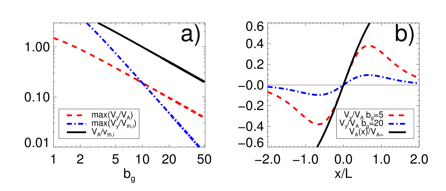
b) Initial profiles of across a CS centered in for two values of guide field, as well as the local Alfvén speed .
The effects of the shear flow need to be carefully considered when normalized to (dependent on ) or (independent on ). The ratio between these two speeds is shown in Fig. 7(a), decreasing with according to the normalization used (see Appendix A). This speed ratio plays an essential role in the GK model, because of the perpendicular drift approximation. This is the assumption that the perpendicular bulk velocities are caused only by the , diamagnetic and other similar drifts. The perpendicular approximation breaks down when the in-plane speeds are close to the ion thermal speeds, such as the typically obtained in magnetic reconnection outflows when . It can also be violated by the presence of waves with high enough frequency (possibly only captured by the fully kinetic plasma description), leading to a cross-field diffusion of particles across the magnetic field.Chen, Le, and Fok (2015) Therefore, deviations from the real physical behavior of a Vlasov plasma modeled via PIC simulations are expected in the GK approach when the ratio . This is precisely the situation when comparing the GK to PIC simulations with or (the latter is the critical guide field for which ).
V.2 Current/flows in secondary magnetic islands
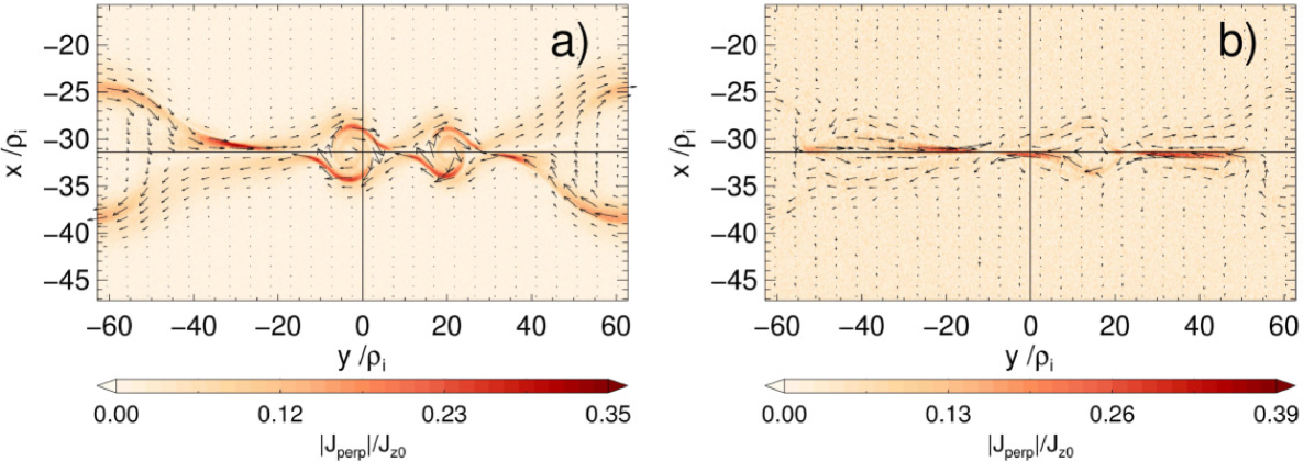
As a result of the initial shear flow, PIC runs with sufficiently low guide field build up a net vortical current inside of the secondary magnetic islands and the periodic boundaries, as can be seen in Fig. 8. The formation of secondary magnetic islands wraps up magnetic field lines around them, deflecting the electron shear flow in the same direction. Therefore, a net out-of-plane magnetic field is generated (see Fig. 3). Note that the direction of the curl of coincides with the direction of the out-of-plane magnetic field ( direction points into the page). As expected, there is a working dynamo process in these places, i.e.: , involving a transfer of energy from the bulk electron motion to the magnetic field (plots not shown here). High guide field PIC or GK runs do not show this effect. (Negative values of are seen only near the outflows, due to the bulk motion of the plasma.) A comparison of this process to the dissipation close to the X points will be given in a follow-up paper.
Two other consequences of the shear flow in reconnection found in previous works are worth to mention in this point. First, the tilting of magnetic islands and generation of concentric vortical flows inside of them as result of sub-Alfvénic flows (in agreement with our parameter regime) has been seen in both 2D MHD and Hall-MHD simulations (see Ref. Shi et al., 2005 and references therein). Second, the increasing symmetry of the core magnetic field for low PIC can also be explained due to the shear flow, as investigated via a two fluid analysis of tearing mode with shear flow of Ref. Hosseinpour and Mohammadi, 2013. But there is also opposite evidence to this claim: Ref. Karimabadi et al., 1999 found, by means of hybrid simulations of Harris sheets, that the “S” shape of in the secondary magnetic islands is only consequence of guide field reconnection (nothing to do with shear flow). This might be due to the small guide field regime analyzed: , not being correct to be applied for our case.
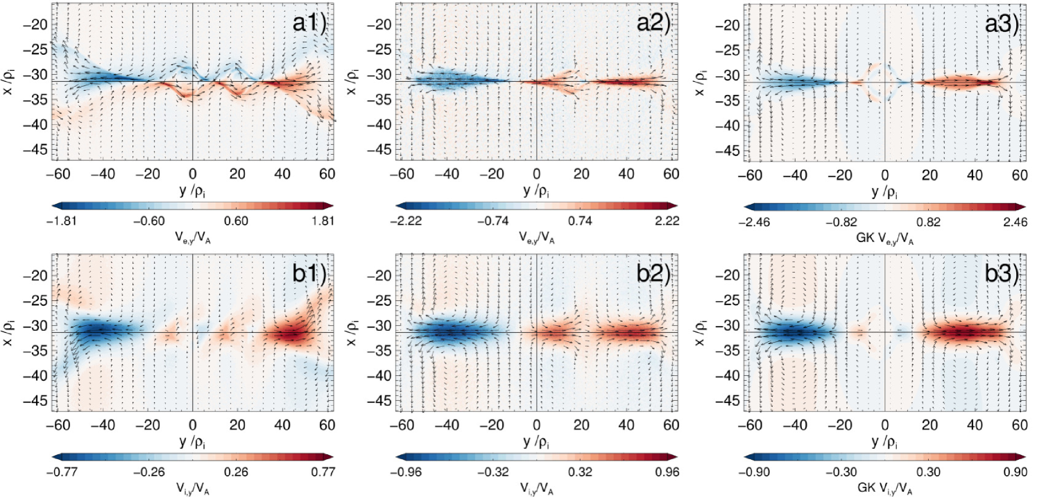
The current inside of the magnetic islands, significant only in the low guide field regime, is produced due to the Hall effect: a decoupling of motion between electrons and ions, as shown in Fig. 9. For the lowest PIC guide field run , the ions follow the outflow due to reconnection from the X point (Fig. 9(b1)), but the electrons keep their initial shear flow and are only weakly deflected (Fig. 9(a1)) by that reconnection outflow, following a vortical flow pattern inside of the magnetic islands. This characteristic (antisymmetric) flow pattern is barely visible for a higher guide field of (see Figs. 9(a2)-(b2)) and totally absent for the GK run (see Figs. 9(a3)-(b3)), where the internal flow has a symmetric structure following the features of the reconnection outflow.
It is important to mention that because the generation of magnetic field is due to a Hall effect, their effects will be stronger when the CS is on the order of/thinner than , the sound Larmor radius (for ), which applies very well to our case (). Therefore, in thicker CS these effects should be significantly reduced and an agreement between PIC and GK simulations of magnetic reconnection will be more easily reached. Note that the halfwidth is also on the order of electron skin depth, since , and so the electron inertial effects are important:Nakamura, Fujimoto, and Otto (2008) electrons are also unmagnetized (not fulfilling the frozen-in condition) for distances .
In Fig. 9, we can estimate that the speed of the electron outflows from the main X point is a few times the asymptotic Alfvén speed . It varies weakly with the guide field in the PIC runs. On the other hand, the ion outflow speeds only reach sub-Alfvénic values , and are much more constant among different PIC guide fields and the GK runs. These values agree, to a first order, with a two fluid theory of magnetic reconnection by Shay et al. (2001): the outflow speeds from the X point should be of the order of the in-plane Alfvén speed for ions and in-plane electron Alfvén speed for electrons. But the initial shear flow is of course strongly dependent on the guide field (see Fig. 7). The combination of both effects determines the critical PIC guide field for which the shear flow can generate the current that builds up the core magnetic field ().
V.3 Time evolution of the current and magnetic field generation
Since in Sec. V.2 we showed that the electron/ion outflows do not depend strongly on when normalized to , the in-plane current will display similar values among different PIC when the same normalization is used, as can be seen in Fig. 8. But according to the Ampère’s law, the generation of depends on the unnormalized , changing with according to Eq. (16). It can be estimated by approximating the curl by the gradient scale length :
| (10) |
Since practically does not change for different PIC guide fields (result of choosing an invariant , recall Sec. II), by defining the constant we infer that (in order of magnitude), when , not dependent on the guide field. Note that this estimate relies on the fact that is approximately constant during the evolution, which in turn depends on the fact that does not have to change too much. We checked that the ion temperature does not increase more than of its initial value throughout the evolution of the system, and therefore we can safely take and so constant for our purposes. This is equivalent to a proportionality between and , a relation always satisfied in a force free equilibrium. This is a valid first order approximation since the magnetic islands grow at ion time scales (), and therefore, at electron time-scales that relation can be satisfied quasi-adiabatically. On the other hand, in our runs can be estimated as the size across the direction of either the secondary magnetic islands close to the point (), or the magnetic island at the boundaries (). Thus, the time history of the maximum value of both components of is shown in Fig. 10.
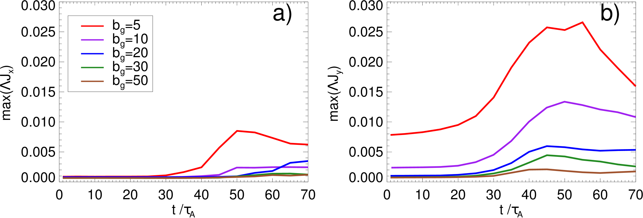
The presence of the initial due to the shear flow can be seen in Fig. 10(b), increasingly important for lower PIC guide fields. But the in-plane component , and to a lesser extent , start to grow just after the formation of secondary magnetic islands. There is a good agreement (in order of magnitude) of the maximum values that reach with the corresponding maximum values of (see Fig. 5(b)) for different guide fields, justifying empirically our estimation Eq. (10). Note that the factor should be removed in the latter for a proper comparison (e.g., for , the maximum is ). It is also important to remark that the maximum values of are reached in the boundaries of the locations where peaks: around the secondary magnetic islands and the boundaries (neglecting the region in the separatrices with almost zero curl). The most important conclusion that can be inferred from Fig. 10 is that the maximum values of , and so , become negligible in the PIC higher guide field limit when measured in absolute units. Therefore, magnetic field generation is only effective in the PIC low guide field regime.
In principle, another possibility for the core-magnetic field generation that it is interesting to analyze is due to a pinch effect and the associated magnetic flux compression inside of the magnetic islands (via conservation of magnetic flux/frozen-in condition). We checked that the divergence for both electrons and ions has a complex spatial structure and mostly odd symmetry inside and around the islands, not correlating well with the properties of (plots not shown here). Moreover, we checked that the absolute value of (normalized to the natural time scale ), is reduced for higher guide fields, implying a more incompressible plasma. This is consequence of the fact that the lowest order perpendicular drifts are incompressible, a condition satisfied better in this regime. However, decays much faster with the guide field as the core-field: already for , this quantity is comparable with the noise level but, on the other hand, there is still significant in the islands for this guide field case. Therefore, a pinch effect is not likely to be responsible for the generation of in the magnetic islands.
All these are indications that the generation of the core magnetic field is due to a combination of the effects of the shear flow and the formation of magnetic islands, becoming increasingly important for lower PIC guide fields, and that is why it should not be taken into account when comparing PIC with GK simulations of magnetic reconnection.
V.4 Effects of counterstreaming outflows in core magnetic field generation
We already mentioned that in the PIC low guide regime, besides of the secondary magnetic islands, a core magnetic field is also generated in the boundaries. This is due to a combination of two mechanisms. The main one is because of the compression by the colliding outflows generated from reconnection in the main X point and the periodic boundary conditions (equivalent to a configuration with multiple X points). This effect is stronger for PIC low guide field regime since the electron outflows are faster (in absolute units, since they have same values in units of ). Note that this process could be avoided by choosing longer boxes.Karimabadi et al. (1999) The second mechanism contributing to the core magnetic field generation is the same as for the secondary magnetic islands, since the O point of the primary magnetic island is located precisely at the boundaries.
V.5 Influence of shear flow in reconnection
As we can see in Fig. 1, the reconnection rates are smaller for the lower guide field cases and compared to the PIC high guide field regime or the GK runs. This can be understood in terms of three different reasons. First, the outflows from the X points should be less efficient (slower) because of the additional magnetic pressure due to in the secondary magnetic islands (and boundaries), after being normalized to the Alfvén speed. This process tends to inhibit the CS thinning. Note that this additional out-of-plane guide field has higher relative importance with respect to the asymptotic magnetic field precisely in cases with low PIC (see, e.g., Fig. 5). Second, as indicated in Ref. Cassak, 2011 with the Hall-MHD model without guide field, the magnetic tension in the reconnected magnetic field lines should be released by the shear flow, reducing the outflow speed produced by them and thus decreasing reconnection rates by a factor of . Similarly, numerical solutions of a kinetic dispersion relation and 2D PIC simulations for thin CSRoytershteyn and Daughton (2008) demonstrated a reduction in the growth rate of the collisionless tearing mode for increasing shear flows, the instability associated with the onset of magnetic reconnection. And third, part of the available magnetic energy for reconnection that should be converted into particle energy is given back when the Hall currents are formed in the secondary magnetic islands. Overall, these reasons suggest that reconnection rates might be reduced in the PIC low guide field regime, if the total plasma is kept constant.
VI Finite plasma beta effects
Let us finally discuss the high beta case with . Although the basic phenomenology of magnetic reconnection and secondary magnetic islands is similar, in general, the agreement is better between different guide field PIC runs in the range and the corresponding GK results. This can be seen in the reconnection rates of Fig. 1(b), as well as in the time evolution of the scaled magnetic fluctuations shown in Fig. 11(b). The time evolution of the thermal pressure fluctuations in Fig. 11(a) displays a different behavior between the results given by both codes. As we already pointed out, the physical origin of these differences will be analyzed in a follow-up paper.
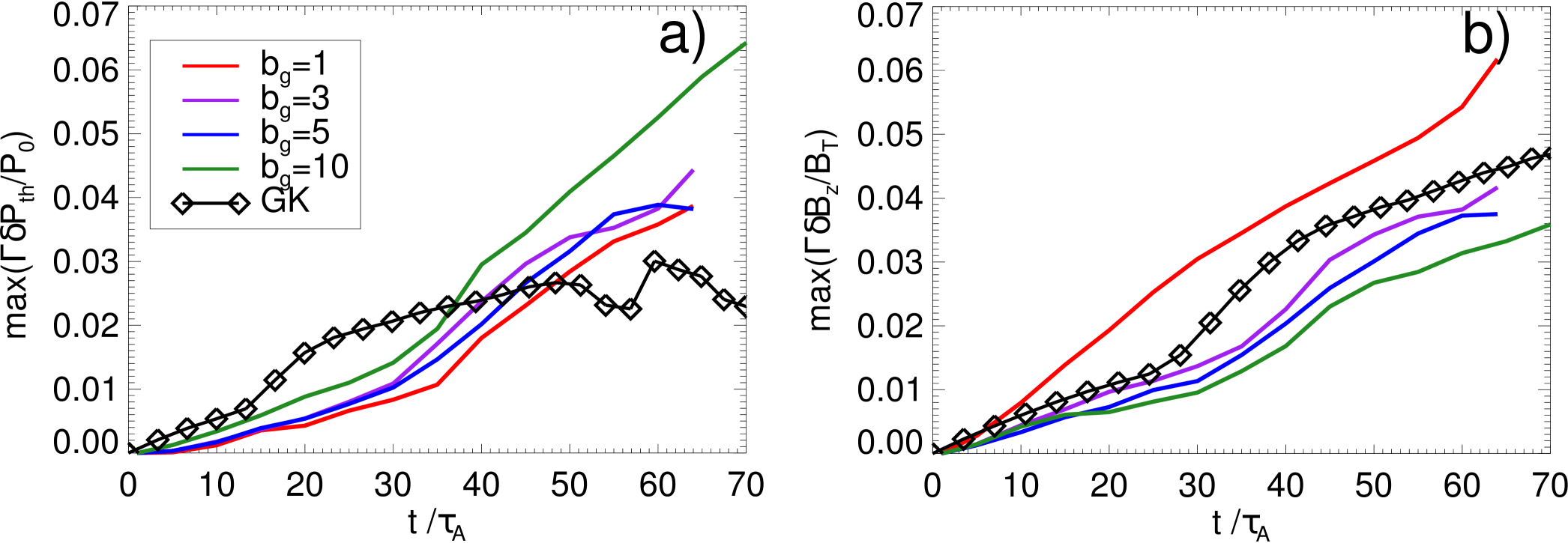
There are at least two related reasons for the better agreement. The first one is because the fluctuations are predicted to be smaller by one order of magnitude compared to the low beta case, since they are proportional to (see Eqs. (5) and (6)). In addition, the GK ordering parameter will also be reduced (see discussion of Eq. (15)), from for in the low beta case to for in the high beta case. This improves the validity of the predictions of the GK compared to the PIC model in this parameter regime, since the largest deviations from the pressure equilibrium condition Eq. (7) will be reduced by the same amount. Also note that the maximum net force due to the total pressure imbalance will be much smaller than in the low beta case.
Second, the range of variation of the speed ratio given by Eq. (16) decreases by a small amount in comparison to the low beta case: going from . This implies that the maximum values of the initial shear flow (for ) are much smaller: , and so are their effects on the system. Moreover, reconnection rates are reduced by a factor of two in this regime (see Fig. 1(b)). Then, the maximum electron/ion outflows speeds in units of , proportional to the reconnection rates, will also be further reduced in comparison to the low beta case, becoming negligible when measured in units of . More precisely, we measured maximum electron outflows speeds on the order of (see Fig.12(3rd. row)) and ion outflows on the order of (see Fig.12(4th. row)), roughly smaller by a factor of 3 compared with the corresponding values in the low beta case.
This reduction in the maximum in-plane flow speeds has two physical consequences. For the GK model, the maximum deviations from the drift approximation will be smaller than in the low beta case (see discussion in Sec. V.1). For the fully kinetic approach, the magnetic field generation due to the colliding outflows at the boundaries is reduced. On the other hand, we also observed smaller magnetic islands in this case, implying a smaller core-magnetic field. This is because the generation of , according to the estimate Eq. (10), is proportional to the length scale of these islands, which is roughly five times smaller compared to the low beta case. This is valid even though the Hall term and the corresponding decoupling of electrons and ions is facilitated in high plasma beta environments, implying a greater in-plane (twice as high compared to the low beta case). The net result of all these effects can be seen in the time evolution of in Fig. 11(b), where the deviations of PIC results compared to the GK ones are significant only for and much smaller in absolute terms compared with the low beta case. Convergence with the GK results is already reached with values (see, e.g., the second column of Fig. 12 for ). This reduction of core magnetic field strength in high plasmas is in agreement with previous hybrid simulationsKarimabadi et al. (1999) (although for very low guide fields ).
Finally, it is important to mention that there is, in general, a higher level of numerical noise, and associated numerical heating, in this high beta case compared to the low beta one for the PIC runs. It becomes increasingly important for higher guide fields, reducing even faster the signal-to-noise ratio. This is, in part, responsible for the monotonically increasing thermal pressure fluctuations in Fig. 11(a) for later times, especially in the case . This observation was already pointed out in Ref. TenBarge et al., 2014, being a well known consequence of the enhanced numerical collisions in weakly magnetized environments simulated by PIC codes, or equivalently, in high beta plasmas.Matsuda and Okuda (1975)
VII Conclusions
We have carried out a comparison of magnetic reconnection in the limit of strong guide field between two plasma models by using fully kinetic PIC with gyrokinetic simulations of force free current sheets. Our study extends the previous work of Ref. TenBarge et al., 2014. We established the limits of applicability of the gyrokinetic approach compared to the fully kinetic model in the realistic regime of finite PIC guide fields, and the physical reasons behind these differences. Note that the following conclusions are based on sets of runs with total ion plasma constant for different PIC guide fields.
First, by using an independent set of PIC and gyrokinetic codes, we found the limitations in the linear scaling reported in Ref. TenBarge et al., 2014 in both thermal and magnetic fluctuations. PIC simulations in the low guide field regime show deviations in the inverse scaling with the guide field, not converging properly to the gyrokinetic results. These deviations start to be especially significant when secondary magnetic islands start to form, after the reconnection peak time. In this paper, we focus on the additional magnetic fluctuations revealed by the PIC low guide field runs, which are mostly due to macroscopic bulk plasma motions. The analysis of the differences in the thermal fluctuations—that have to do with dissipative processes, heating mechanisms and non thermal effects—will be addressed in a follow-up paper.
In particular, we found that the PIC low guide field regime shows an excess of magnetic pressure inside of the secondary magnetic islands (core magnetic field), reaching maximum values for times much later than the reconnection peak time. Correspondingly, the agreement between the two plasma descriptions is better before the formation of these structures, during the linear phase of magnetic reconnection. This excess of magnetic pressure is not compensated by a corresponding decrease in the thermal pressure. The reason is that gyrokinetic codes keep the pressure equilibrium condition to machine precision because perpendicular force balance is enforced in the GK equations, while PIC codes allow large deviations from it since they solve the full collisionless Vlasov-Maxwell system of equations. Therefore, although the gyrokinetic results can be comparable to the PIC ones for relatively low guide fields ( and ) in the separatrices close to the X points, convergence in the secondary magnetic islands requires much higher guide fields ().
We found that the physical mechanism that generates the core magnetic field (associated with a dynamo effect ) is due to an initial shear flow present in the force free PIC initialization. This shear flow, that also produces asymmetric separatrices and reduces reconnection rates, is negligible in the limit of strong guide field and absent in the corresponding gyrokinetic initialization. Through the Hall effect that decouples electron from ion motion, vortical electron flow patterns are generated in the secondary magnetic islands as magnetic reconnection wraps up magnetic field lines around these structures, carrying the electron shear flow with them. This magnetic field weakens for higher PIC guide field runs, converging to the gyrokinetic result, since the shear flow is not strong enough to drive the currents capable of generating it (when measured in absolute units). There is also an out-of-plane magnetic field generation at the periodic boundaries, where it is located at the O point of the primary magnetic island. This is not only due to the same previous mechanism, but also due to the compression by colliding electron outflows, faster in the PIC runs with low guide field (in absolute units).
We also showed that the relative ratio of the electron outflow speed to the ion thermal speed, proportional to , is higher for the PIC low guide field regime, reaching values close to 1 for . This breaks the perpendicular drift approximation, a critical assumption in which the gyrokinetic codes (and the gyrokinetic theory in general) are based, and thus an additional source of differences is expected compared to the PIC simulation results.
Finally, we also analyzed the effects of a high plasma beta compared to our standard case . Although the basic phenomenology is similar, we could notice a better agreement between the corresponding PIC and gyrokinetic results, reaching a relatively good convergence for guide fields as low as . From this, we can conclude that an accurate comparison between PIC and gyrokinetic force free simulations of magnetic reconnection requires high plasma (to reduce the fluctuation level proportional to ), although PIC codes are affected by enhanced numerical heating in this regime. Moreover, it is necessary to have parameters with low ratios (to avoid the effects of the initial shear flow), a small ordering parameter in the gyrokinetic initialization, and reconnection rates should not be too high . In the PIC model, this is to avoid super-Alfvénic outflows generating stronger magnetic fields at the periodic boundaries, while in gyrokinetic model these flows might also break the perpendicular drift approximation. The balance of these related numerical and physical parameters allow to determine a convenient parameter regime for an accurate comparison of magnetic reconnection between these plasma models.
In spite of all those differences, the gyrokinetic simulations show a development of magnetic reconnection remarkably similar to the PIC high guide field runs. This is of central importance due to the computational savings of the first ones. Indeed, for the low beta case, we measured speed-ups by a factor of between the gyrokinetic runs compared to a corresponding PIC guide field simulation. However, the computational cost of a PIC simulation decreases linearly with the guide field, in such a way that in the low guide field regime (), the speed-up and advantages of using gyrokinetic instead of PIC simulations are not so notorious.
Acknowledgements.
We acknowledge the developers of the code ACRONYM at Würzburg University, the support by the Max-Planck-Princeton Center for Plasma Physics and of the German Science Foundation DFG-CRC 963 for P. K and J. B. P. M. acknowledges the financial support of the Max-Planck Society via the IMPRS for Solar System Research. The research leading to these results has received funding from the European Research Council under the European Union’s Seventh Framework Programme (FP7/2007-2013)/ERC Grant Agreement No. 277870. All authors thank the referee for valuable and constructive comments which helped us to verify our results and to make our points more clear.Appendix A Normalizations
Here, we explained all the details regarding normalization and the right choice of a correspondence between the GK and PIC results.
The lengths are normalized to and the times to the Alfvén time , where is the Alfvén speed defined with respect to the reconnected magnetic field
| (11) |
where is the electron plasma frequency. We use the previous definitions for the normalization of the reconnection rate: and current density: . Note that due to the Ampère’s law, the normalized initial out-of-plane current density that supports the asymptotic magnetic field is given by:
| (12) |
which is independent on the guide field strength.
As we mentioned in Sec. III.2, many of the fluctuating quantities scale with the guide field due to the fact that , and so the transverse distance , are constant for different (with the last claim proved in Appendix B). Therefore, the PIC fluctuating quantities will have the same value under the previous assumption if they are multiplied by the factor proportional to
| (13) |
where is a reference guide field, chosen to be in the low/high beta case, respectively. The value in the low beta case was chosen because the respective runs are not so dominated by numerical noise as for larger guide fields () and so it is easier to compare with the noiseless GK runs. In addition, is not in the lowest end of guide fields like where other effects not captured by GK (explained in the results, Secs. III, IV and V), dominate the physics of the system. In this way, using Eqs. (13) and (5), the quantity that should be equal among different guide field PIC runs is
| (14) |
and analogously for . The factor instead of is in order to keep the total magnetic field constant (and not only ).
On the other hand, the definition of in Eq. (13) also fixes the ordering parameter of the GK runs, defined by:
| (15) |
where is the normalized asymptotic magnetic field with respect to a reference value expressed in code units. The initialization in the GK runs gives for the low/high beta cases, respectively. Therefore, using the aforementioned PIC , we have for the low/high beta case, respectively. Note that even though in the low beta plasma regime with the GK ordering formally does not hold, and in agreement with Ref. TenBarge et al., 2014, this plasma model can still make accurate predictions, but only under some circumstances (clarified in the results, Secs. III, IV and V). Moreover, the unusually high value of is required to have a perturbed current strong enough to generate the relative large perturbed asymptotic magnetic field for the case (being reduced for higher guide fields).
The choice of a constant for different guide fields has another important consequence for the ratio of Alfvén to ion thermal speed. Indeed, due to that assumption, the PIC runs will invariably have to change this parameter for different guide fields
| (16) |
Note that is constant for different guide fields, while scales inversely with it. This means that the ratio increases for lower PIC guide fields: from going from in the low beta case.
It is also important to mention another side effect of the normalization used (already noticed in Ref. TenBarge et al., 2014). Since decreases for increasing , it becomes more comparable to the noise level for very high . Then, for large the signal-to-noise ratio of all the fields can be very low, as can be seen in the extreme case in Fig. 2(e) and Fig. 3(e) (even with the extended temporal average). Therefore, although in principle there is no limitation due to numerical constraints on the electron gyromotion for even higher guide fields (in our setup, and are constant for different guide fields), the PIC results in this regime are not reliable due to this unfortunate fact.
Appendix B Transverse distance
Here, we proved the statement written in Sec. III.2: the transverse distance of the thermal and magnetic fluctuations scale as . This implies: (1) it is constant for different guide fields (requirement for the inverse scaling with ) and (2) it is higher for the high than the low beta set of parameters. We estimated the value of shown in Fig. 13 by using the plots of in Fig. 2. First, we detected the main X point by locating the minimum of the vector potential along the center of the CS. Then, we chose several distances to the left of that point in the direction along the center of the CS (, indicated in the axis of Fig. 13). From each point we measured the transverse distance across the direction, , from the center until the point in which the current density drops to and of its initial peak value, as a simple way to detect the boundaries of the CS in these regions (averaging in both positive and negative directions). These values correlate well enough with the approximate boundaries of the regions with significant values of (as well as ) above numerical noise, besides of being independent of scaling arguments. The small error bars are the differences between the and of the initial value of .
First of all, in Fig. 13(left) we can see that for the low beta case, the transverse distance is more or less constant for different guide fields at least for (longitudinal) distances away from the main X point, confirming the assumption stated before. As can be expected, the transverse distance increases away from the X point, consequence of the more open separatrices but also because the distinction between them and the boundary of the main magnetic island is more diffuse. In this region, there are more deviations from the previous constant trend for among different guide fields, but in any case, they are not significant, and a value , corresponding to 3 times the order of magnitude estimate , can be considered representative not too far away from the X point. Note that the deviations from more or less constant values are specially significant for the cases of higher guide field or , since the structures of the separatrices away from the X point and close to the O points are different from the low guide field cases (see Fig. 2). On the other hand, the estimations for the transverse distance for the high beta case in Fig. 13(right) show larger variations among guide fields, since in many cases the CS develop small secondary islands to the left and very close of the main X point and so the measurement is biased. In addition, for this high beta case, the enhanced level of numerical noise makes the detection of the transverse distance more inaccurate. For this case, it is only possible to conclude that the transverse distance is in between a certain range with a spread of . Nevertheless, close enough to the X point (), can still be considered reliable enough for a comparison (excluding the extreme case ). This value turns out to be practically, in order of magnitude, the estimate .
Therefore, from the results shown in Fig. 13, we can confirm that is (1) more or less constant for different guide fields, especially in the low beta case, and (2) its order of magnitude is between 1-3 times , which is good enough to ensure the validity of the inverse scaling with of and . Note that if we had chosen to keep constant and increase to have a higher guide field effect, the total would not be constant and so the inverse scaling, implying that a direct comparison between the different PIC guide fields and GK runs would not be possible.
Appendix C Computational performance of the GK/PIC codes
It is worthwhile to mention the speed-up of the GK simulations compared to the PIC runs, the main motivation of using the first numerical method over the second one for magnetic reconnection studies. Because of the choice of keeping the total plasma constant for different PIC guide fields to properly compare with the GK results (see Appendix A), the Alfvén time in units of is (practically) linearly proportional to according to
| (17) |
In the PIC runs, because the time step has to be proportional to for stability reasons, the latter expression will also be proportional to the number of time steps used to reach a given time measured in , and thus to the computational effort. Then, PIC high guide field runs are computationally more expensive than the runs in the low guide field regime (as well as the high beta cases compared to the low beta ones). In fact, for the low beta case, the ACRONYM PIC code used CPU core-hours to run the cases up to (the last time shown in Fig. 1), while CPU core-hours for the case . A significant fraction of this computational effort is spent in running time diagnostics for higher order momenta of the distribution function, which are used in the results to be shown in a follow-up paper. On the other hand, the single GENE GK code simulation with which those runs were compared used only CPU core-hours, representing a speed-up by a factor of when comparing with the largest PIC guide field considered . These huge computational savings are an additional justification for the importance of a proper comparison study of GK with PIC simulations of guide field reconnection, one of the purposes of the present paper.
References
- Büchner (2007) J. Büchner, Plasma Phys. Control. Fusion 49, B325 (2007).
- Zweibel and Yamada (2009) E. G. Zweibel and M. Yamada, Annu. Rev. Astron. Astrophys. 47, 291 (2009).
- Yamada, Kulsrud, and Ji (2010) M. Yamada, R. M. Kulsrud, and H. Ji, Rev. Mod. Phys. 82, 603 (2010).
- Treumann and Baumjohann (2013) R. A. Treumann and W. Baumjohann, Front. Phys. 1, 31 (2013), arXiv:1401.5995 .
- Büchner, Dum, and Scholer (2003) J. Büchner, C. Dum, and M. Scholer, Space Plasma Simulation (Springer-Verlag, Berlin Heidelberg, 2003).
- Frieman and Chen (1982) E. A. Frieman and L. Chen, Phys. Fluids 25, 502 (1982).
- Brizard and Hahm (2007) A. J. Brizard and T. S. Hahm, Rev. Mod. Phys. 79, 421 (2007).
- Howes et al. (2006) G. G. Howes, S. C. Cowley, W. Dorland, G. W. Hammett, E. Quataert, and A. a. Schekochihin, Astrophys. J. 651, 590 (2006).
- Schekochihin et al. (2009) A. A. Schekochihin, S. C. Cowley, W. Dorland, G. W. Hammett, G. G. Howes, E. Quataert, and T. Tatsuno, Astrophys. J. Suppl. Ser. 182, 310 (2009).
- Wan, Chen, and Parker (2005) W. Wan, Y. Chen, and S. E. Parker, IEEE Trans. Plasma Sci. 33, 609 (2005).
- Rogers et al. (2007) B. N. Rogers, S. Kobayashi, P. Ricci, W. Dorland, J. Drake, and T. Tatsuno, Phys. Plasmas 14, 092110 (2007).
- Pueschel et al. (2011) M. J. Pueschel, F. Jenko, D. Told, and J. Büchner, Phys. Plasmas 18, 112102 (2011).
- Pueschel et al. (2014) M. J. Pueschel, D. Told, P. W. Terry, F. Jenko, E. G. Zweibel, V. Zhdankin, and H. Lesch, Astrophys. J. Suppl. Ser. 213, 30 (2014).
- Harris (1962) E. G. Harris, Nuovo Cim. 23, 115 (1962).
- TenBarge et al. (2014) J. M. TenBarge, W. Daughton, H. Karimabadi, G. G. Howes, and W. Dorland, Phys. Plasmas 21, 020708 (2014), arXiv:1312.5166 .
- Rogers, Denton, and Drake (2003) B. N. Rogers, R. E. Denton, and J. F. Drake, J. Geophys. Res. 108, 1111 (2003).
- Roach et al. (2005) C. M. Roach, D. J. Applegate, J. W. Connor, S. C. Cowley, W. D. Dorland, R. J. Hastie, N. Joiner, S. Saarelma, A. A. Schekochihin, R. J. Akers, C. Brickley, A. R. Field, M. Valovic, and t. M. Team, Plasma Phys. Control. Fusion 47, B323 (2005).
- Abel et al. (2013) I. G. Abel, G. G. Plunk, E. Wang, M. Barnes, S. C. Cowley, W. Dorland, and A. A. Schekochihin, Reports Prog. Phys. 76, 116201 (2013), arXiv:1209.4782 .
- Chen, Daughton, and Bhattacharjee (2012) L. Chen, W. Daughton, and A. Bhattacharjee, Phys. Plasmas 19, 112902 (2012).
- Zhou, Deng, and Huang (2012) M. Zhou, X. H. Deng, and S. Y. Huang, Phys. Plasmas 19, 042902 (2012).
- Huang et al. (2014) S. Y. Huang, M. Zhou, Z. G. Yuan, X. H. Deng, F. Sahraoui, Y. Pang, and S. Fu, J. Geophys. Res. Sp. Phys. 119, 7402 (2014).
- Huang et al. (2013) C. Huang, Q. Lu, M. Wu, S. Lu, and S. Wang, J. Geophys. Res. Sp. Phys. 118, 991 (2013).
- Drake et al. (2006) J. F. Drake, M. Swisdak, K. M. Schoeffler, B. N. Rogers, and S. Kobayashi, Geophys. Res. Lett. 33, L13105 (2006).
- Daughton et al. (2011) W. Daughton, V. Roytershteyn, H. Karimabadi, L. Yin, B. J. Albright, S. P. Gary, K. J. Bowers, and S. Consistent, in AIP Conf. Proc., Vol. 1320 (2011) p. 144.
- Karimabadi et al. (1999) H. Karimabadi, D. Krauss-Varban, N. Omidi, and H. X. Vu, J. Geophys. Res. 104, 12313 (1999).
- Zhou et al. (2014) M. Zhou, Y. Pang, X. Deng, S. Huang, and X. Lai, J. Geophys. Res. Sp. Phys. 119, 6177 (2014).
- Cassak (2011) P. A. Cassak, Phys. Plasmas 18, 072106 (2011).
- Roytershteyn and Daughton (2008) V. Roytershteyn and W. Daughton, Phys. Plasmas 15, 082901 (2008).
- Hosseinpour and Mohammadi (2013) M. Hosseinpour and M. A. Mohammadi, Phys. Plasmas 20, 114501 (2013).
- Wang, Pritchett, and Ashour-Abdalla (1992) Z. Wang, P. L. Pritchett, and M. Ashour-Abdalla, Phys. Fluids B Plasma Phys. 4, 1092 (1992).
- Fermo, Drake, and Swisdak (2012) R. L. Fermo, J. F. Drake, and M. Swisdak, Phys. Rev. Lett. 108, 255005 (2012).
- Liu et al. (2014) Y.-H. Liu, W. Daughton, H. Karimabadi, H. Li, and S. Peter Gary, Phys. Plasmas 21, 022113 (2014).
- Loureiro, Schekochihin, and Uzdensky (2013) N. F. Loureiro, A. A. Schekochihin, and D. A. Uzdensky, Phys. Rev. E 87, 013102 (2013).
- Kilian, Burkart, and Spanier (2012) P. Kilian, T. Burkart, and F. Spanier, in High Perform. Comput. Sci. Eng. ’11, edited by W. E. Nagel, D. B. Kröner, and M. M. Resch (Springer Berlin Heidelberg, Berlin, Heidelberg, 2012) pp. 5–13.
- Jenko et al. (2000) F. Jenko, W. Dorland, M. Kotschenreuther, and B. N. Rogers, Phys. Plasmas 7, 1904 (2000).
- Pritchett (2001) P. L. Pritchett, J. Geophys. Res. 106, 3783 (2001).
- Pritchett and Coroniti (2004) P. L. Pritchett and F. V. Coroniti, J. Geophys. Res. 109, A01220 (2004).
- Ricci et al. (2004) P. Ricci, J. U. Brackbill, W. Daughton, and G. Lapenta, Phys. Plasmas 11, 4102 (2004).
- Numata and Loureiro (2014) R. Numata and N. F. Loureiro, in Proc. 12th Asia Pacific Phys. Conf., Vol. 1 (Journal of the Physical Society of Japan, 2014) p. 015044, arXiv:1311.2728v2 .
- Numata and Loureiro (2015) R. Numata and N. F. Loureiro, J. Plasma Phys. 81, 305810201 (2015), arXiv:1406.6456 .
- Rogers et al. (2001) B. N. Rogers, R. E. Denton, J. F. Drake, and M. A. Shay, Phys. Rev. Lett. 87, 195004 (2001).
- Stanier et al. (2015) A. Stanier, A. N. Simakov, L. Chacón, and W. Daughton, Phys. Plasmas 22, 010701 (2015).
- Cassak et al. (2015) P. A. Cassak, R. N. Baylor, R. L. Fermo, M. T. Beidler, M. A. Shay, M. Swisdak, J. F. Drake, and H. Karimabadi, Phys. Plasmas 22, 020705 (2015), arXiv:1502.01781v1 .
- Chen, Le, and Fok (2015) S.-H. Chen, G. Le, and M.-C. Fok, J. Geophys. Res. Sp. Phys. 120, 113 (2015).
- Shi et al. (2005) Q. Q. Shi, Z. Y. Pu, H. Zhang, S. Y. Fu, C. J. Xiao, Q. G. Zong, T. A. Fritz, and Z. X. Liu, Surv. Geophys. 26, 369 (2005).
- Nakamura, Fujimoto, and Otto (2008) T. K. M. Nakamura, M. Fujimoto, and A. Otto, J. Geophys. Res. Sp. Phys. 113, A09204 (2008).
- Shay et al. (2001) M. A. Shay, J. F. Drake, B. N. Rogers, and R. E. Denton, J. Geophys. Res. 106, 3759 (2001).
- Matsuda and Okuda (1975) Y. Matsuda and H. Okuda, Phys. Fluids 18, 1740 (1975).