^†^†institutetext: Kavli Institute for Theoretical Sciences (KITS),
University of Chinese Academy of Sciences (UCAS), Beijing 100190, China

Half-Wormholes and Ensemble Averages

Cheng Peng, Jia Tian and Yingyu Yang pengcheng@ucas.ac.cn, wukongjiaozi@ucas.ac.cn, yangyingyu18@mails.ucas.ac.cn

Abstract

We study “half-wormhole-like” saddle point contributions to spectral correlators in a variety of ensemble average models, including various statistical models, generalized 0d SYK models, 1d Brownian SYK models and an extension of it. In statistical ensemble models, where more general distributions of the random variables could be studied in great details, we find the accuracy of the previously proposed approximation for the half-wormholes could be improved when the distribution of the random variables deviate significantly from Gaussian distributions. We propose a modified approximation scheme of the half-wormhole contributions that also work well in these more general theories. In various generalized 0d SYK models we identify new half-wormhole-like saddle point contributions. In the 0d SYK model and 1d Brownian SYK model, apart from the wormhole and half-wormhole saddles, we find new non-trivial saddles in the spectral correlators that would potentially give contributions of the same order as the trivial self-averaging saddles. However after a careful Lefschetz-thimble analysis we show that these non-trivial saddles should not be included. We also clarify the difference between “linked half-wormholes” and “unlinked half-wormholes” in some models.

1 Introduction

The AdS/CFT correspondence Maldacena:1997re ; Witten:1998qj ; Gubser:1998bc provides a non-perturbative definition of quantum gravity. An important lesson from the recently progress in understanding the black hole information paradox is that a summation of different configurations in the semi-classical gravitational path integral is crucial to probe some quantum mechanical properties of the system, such as the Page curve Penington:2019npb ; Almheiri:2019psf ; Almheiri:2019hni ; Penington:2019kki , the late-time behavior of the spectral form factor Saad:2019lba ; Saad:2018bqo , and correlation functions Saad:2019pqd ; Yan:2022nod , see also a recent review in Bousso:2022ntt . However, the inclusion of spacetime wormholes leads to an apparent factorization puzzle Maldacena:2004rf ; a holographic computation of the correlation functions of field theory partition functions living on different boundaries gives non-factorized results, i.e. $\langle Z_{L}Z_{R}\rangle\neq\langle Z_{L}\rangle\times\langle Z_{R}\rangle$ , which is in tension with the general expectation on the field theory side. This revitalizes the hypothetical connection between wormholes and ensemble averages Coleman:1988cy ; Giddings:1988wv ; Giddings:1988cx ; Polchinski:1994zs , and motivates an appealing conjectural duality between a bulk gravitational theory and (the average of) an ensemble of theories on the boundary Saad:2019lba ; Stanford:2019vob ; Iliesiu:2019lfc ; Kapec:2019ecr ; Maxfield:2020ale ; Witten:2020wvy ; Mefford:2020vde ; Altland:2020ccq ; Eberhardt:2021jvj ; Stanford:2021bhl ; Arefeva:2019buu ; Betzios:2020nry ; Anninos:2020ccj ; Berkooz:2020uly ; Mertens:2020hbs ; Turiaci:2020fjj ; Anninos:2020geh ; Gao:2021uro ; Godet:2021cdl ; Johnson:2021owr ; Blommaert:2021etf ; Okuyama:2019xbv ; Forste:2021roo ; Maloney:2020nni ; Afkhami-Jeddi:2020ezh ; Cotler:2020ugk ; Benjamin:2021wzr ; Perez:2020klz ; Cotler:2020hgz ; Ashwinkumar:2021kav ; Afkhami-Jeddi:2021qkf ; Collier:2021rsn ; Benjamin:2021ygh ; Dong:2021wot ; Dymarsky:2020pzc ; Meruliya:2021utr ; Bousso:2020kmy ; Janssen:2021stl ; Cotler:2021cqa ; Marolf:2020xie ; Balasubramanian:2020jhl ; Gardiner:2020vjp ; Belin:2020hea ; Belin:2020jxr ; Altland:2021rqn ; Belin:2021ibv ; Peng:2021vhs ; Banerjee:2022pmw ; Heckman:2021vzx ; Johnson:2022wsr ; Collier:2022emf ; Chandra:2022bqq ; Schlenker:2022dyo , whose prototype is the by-now well known duality between the two-dimensional Jackiw-Teitelboim (JT) gravity Jackiw:1984je ; Teitelboim:1983ux and the Schwarzian sector of the Sachdev-Ye-Kitaev (SYK) model Sachdev:1992fk ; KitaevTalk2 , or more directly the random matrix theories Saad:2019lba ; Stanford:2019vob . Alternatively, an interesting question is whether there exist other configurations whose inclusion into the gravitational path integral would capture properties of a single boundary theory that are washed out after averaging over the ensemble. This is closely related to the belief that solving the factorization problem will shed light on the microscopic structure of quantum gravity such as the microstates or the states behind the horizon of the black hole; these fine structures are not universal so they can not be captured by the ensemble averaged quantities Stanford:2020wkf ; Almheiri:2021jwq . In Saad:2021uzi , the factorization problem is carefully studied in a toy model introduced in Marolf:2020xie , where it is shown that the (approximate) factorization can be restored if other half-wormhole contributions are included. In the dual field theory analysis, these half-wormhole contributions are identified with non-self-averaging saddle points in the ensemble averaged theories. This idea is explicitly realized in a 0-dimensional “one-time” SYK model in Saad:2021rcu , followed by further analyses in different models Mukhametzhanov:2021nea ; Garcia-Garcia:2021squ ; Choudhury:2021nal ; Mukhametzhanov:2021hdi ; Okuyama:2021eju ; Goto:2021mbt ; Blommaert:2021fob ; Goto:2021wfs . An explicit connection between the gravity computation in Saad:2021uzi and the field theory computation in Saad:2021rcu is proposed in Peng:2021vhs .

The construction of half-wormhole in Saad:2021rcu is based on the $G,\Sigma$ effective action of the model that comes from the Gaussian statistics of the random coupling. Furthermore, a prescription to identify the half-wormhole contribution is proposed and verified for the 0-dimensional SYK model and GUE matrix model in Mukhametzhanov:2021hdi . This raised a question of whether half-wormhole contributions also exist in different ensemble theories, such as those with random variables from a Poisson distribution Peng:2020rno or a uniform distribution on the moduli space Maloney:2020nni ; Afkhami-Jeddi:2020ezh ; Cotler:2020ugk ; Perez:2020klz ; Benjamin:2021wzr ; Dong:2021wot ; Collier:2022emf ; Chandra:2022bqq , and whether these contributions share the same general properties as those discussed in Saad:2021rcu and Mukhametzhanov:2021hdi .

In this paper we study the half-wormhole-like contributions that characterize the distinct behaviors of each individual theory in an ensemble of theories, and test the approximation schemes of the half-wormholes in various models. Our main findings are summarized as follows.

1.1 Summary of our main results

✓

To understand the nature of the half-wormhole contributions in the 1-time SYK model, an approximation scheme is proposed in Mukhametzhanov:2021hdi . Since the proposal does not rely on specific details of the SYK model, such as the collective $G$ and $\Sigma$ variables, it is interesting to understand if there is a similar approximation that applies to more general ensemble averaged theories. In this paper, we first consider various statistical models with a single or multiple random variables. We compute a variety of different quantities, such as simple observables, power-sum observables and product observables, before and after the statistical average. We propose an approximation formula for the half-wormhole like contributions in general statistical models, which generalizes the one in Mukhametzhanov:2021hdi , and show their validity explicitly. We find the validity of the “wormhole/half-wormhole” approximation crucially depend on the large- $N$ factorization property of the observables we consider. The large- $N$ constraints such as traces and determinants play crucial roles in the validity of this approximation.
✓

We review the 0-dimensional SYK model introduced in Saad:2021rcu and fill in technical details of some calculations. In particular, in the saddle point analysis of various quantities, such as $\langle\Phi(\sigma)^{2}\rangle$ and others, we find new non-trivial saddle points whose on-shell values, including the 1-loop corrections, are of the same order as the the trivial saddle that is accounted for the half-wormhole. We then carry out explicit Lefschetz-thimbles analyses to conclude that the contributions from these non-trivial saddle points should not be included in the path integral, which supports the previous results in Saad:2021rcu . We also extend some of the computations to two-loop order and again find our results support previous conclusions in Saad:2021rcu .
✓

We generalize the 0-dimensional SYK model so that the random coupling $J_{i_{1}\dots i_{q}}$ can be drawn from more general distributions, with non-vanishing mean or higher order cumulants.

When $J_{i_{1}\dots i_{q}}$ has a non-vanishing mean value, we find new half-wormhole saddle of $z$ in additional to the linked half-wormhole saddle of $z^{2}$ . We introduce new collective variables $G,\Sigma$ to compute $\langle z\rangle$ and identify the contributions from the half-wormhole saddle. We further consider the half-wormhole proposal in this context. We find that depending on the relative ratio between the different cumulants, different “multiple-linked-wormholes” could be dominant. In particular, in very special limits approximate factorization could hold automatically and no other “half-wormholes” saddles are needed.

In models with non-vanishing higher cumulants of the random coupling, e.g. $\langle J_{i_{1},\dots i_{q}}^{4}\rangle\neq 0$ , we find a similar conclusion that the saddle point contributes. Equivalently, the bulk configurations that dominate the path integral depends crucially on the ratios of the various cumulants and the result is not universal.

In addition, we do a preliminary analysis of models whose random couplings $J_{i_{1},\dots i_{q}}$ are drawn from a discrete distribution, the Poisson distribution, where more complicated saddle points can be found.
✓

We do a similar analysis explicitly to the Brownian SYK model, and identify the wormhole and half-wormhole saddles at late time. The results are computed from both an explicit integration and a saddle point analysis, and we find a perfect agreement between them. We test the approximation of the partition function by its mean value and the half wormhole saddle, and further show that this approximation is good by demonstrating that the error of this approximation is small. Interestingly, like in the 0-dimensional model we also find non-trivial saddles for $\langle\Phi(\sigma)^{2}\rangle$ and they should be excluded by a similar Lefschetz thimble analysis.
✓

We further investigate modified 0d and 1d SYK model whose random couplings have non-vanishing mean values that are written in terms of products of some background Majorana fermions Goto:2021wfs . We compute explicitly the wormhole and a new type of saddle point, the “unlinked half-wormholes”, that contribute to the partition function. We show these unlink half-wormholes are closely related to the disconnected saddles due to the non-vanishing mean value of the random coupling.

2 Statistical models

In this section we consider statistical models, which can be considered as toy models of the Random Matrix Theories, to test the idea of half-wormholes in ensemble theories with random variables drawn from different distributions.

2.1 Models of a single random variable

Let $X$ be a random variable with a PDF $P(X)$ that satisfies the inequality

\displaystyle\langle X^{2}\rangle\geq\langle X\rangle^{2}\,,

(1)

that is valid for all conventional probability distributions. To identify the “half-wormhole contributions” in this model, we consider the unaveraged observable $X$ , $X^{2}$ etc., and rewrite

\displaystyle X^{n}

\displaystyle=\int dx\,\delta(x-X)\frac{x^{n}P(x)}{P(X)}=\int dx\int\frac{dk}{2\pi}\,e^{\text{i}k(x-X)}\frac{x^{n}P(x)}{P(X)}=\int\frac{dk}{2\pi}\frac{e^{-\text{i}kX}}{P(X)}\langle x^{n}e^{\text{i}kx}\rangle\,,

(2)

where as usual the angle bracket denotes the average of $x$ with the probability distribution $P(x)$

\displaystyle\langle\mathcal{O}e^{\text{i}kx}\rangle=\int dx\,\mathcal{O}e^{\text{i}kx}P(x)\ .

(3)

Such expectation values can further be decomposed into the connected and disconnected parts, for example

	$\displaystyle\langle xe^{\text{i}kx}\rangle=\langle x\rangle\langle e^{\text{i}kx}\rangle+\langle xe^{\text{i}kx}\rangle_{\text{c}}\,,$		(4)
	$\displaystyle\langle x^{2}e^{\text{i}kx}\rangle=\langle x^{2}\rangle\langle e^{\text{i}kx}\rangle+2\langle x\rangle\langle xe^{\text{i}kx}\rangle_{c}+\langle x^{2}e^{\text{i}kx}\rangle_{\text{c}},$		(5)
	$\displaystyle\langle x^{3}e^{\text{i}kx}\rangle=\langle x^{3}\rangle\langle e^{\text{i}kx}\rangle+3\langle x^{2}\rangle\langle xe^{\text{i}kx}\rangle_{c}+3\langle x\rangle\langle x^{2}e^{\text{i}kx}\rangle_{c}+\langle x^{3}e^{\text{i}kx}\rangle_{\text{c}}\,,$		(6)
	$\displaystyle\dots$

where the subscript $c$ denotes “connected” or “cumulant” which can be defined recursively as

	$\displaystyle\langle xe^{\text{i}kx}\rangle_{\text{c}}=\langle xe^{\text{i}kx}\rangle-\langle x\rangle\langle e^{\text{i}kx}\rangle,$		(7)
	$\displaystyle\langle x^{2}e^{\text{i}kx}\rangle_{\text{c}}=\langle x^{2}e^{\text{i}kx}\rangle-\langle x^{2}\rangle\langle e^{\text{i}kx}\rangle-2\langle x\rangle\langle xe^{\text{i}kx}\rangle_{\text{c}},$		(8)
	$\displaystyle\dots$

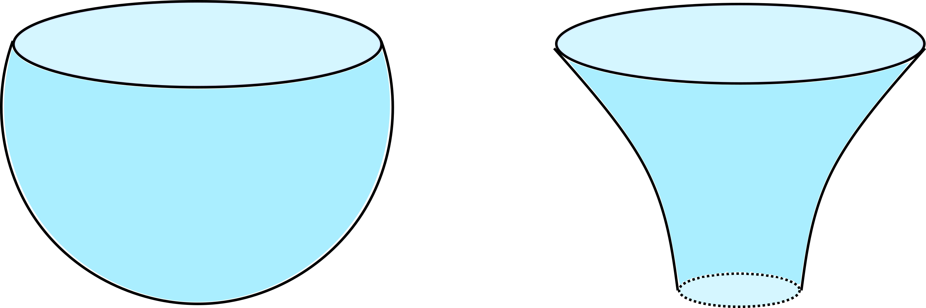
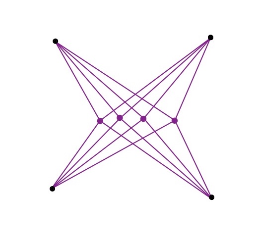
There is a diagrammatic way to understand this result that closely resembles the 2-dimensional topological gravity model which is introduced in Marolf:2020xie . Formally writing

\displaystyle\langle\mathcal{O}e^{\text{i}kx}\rangle=\langle\mathcal{O}|e^{\text{i}kx}\rangle,

(9)

we can interpret the state $|e^{\text{i}kx}\rangle$ as a “spacetime” D-brane ${}_{\text{i}k}$ state that is similar to that introduced in Marolf:2020xie . Then the relation (5) can be understood as in Figure 1 where the meaning of the subscript $c$ is transparent.

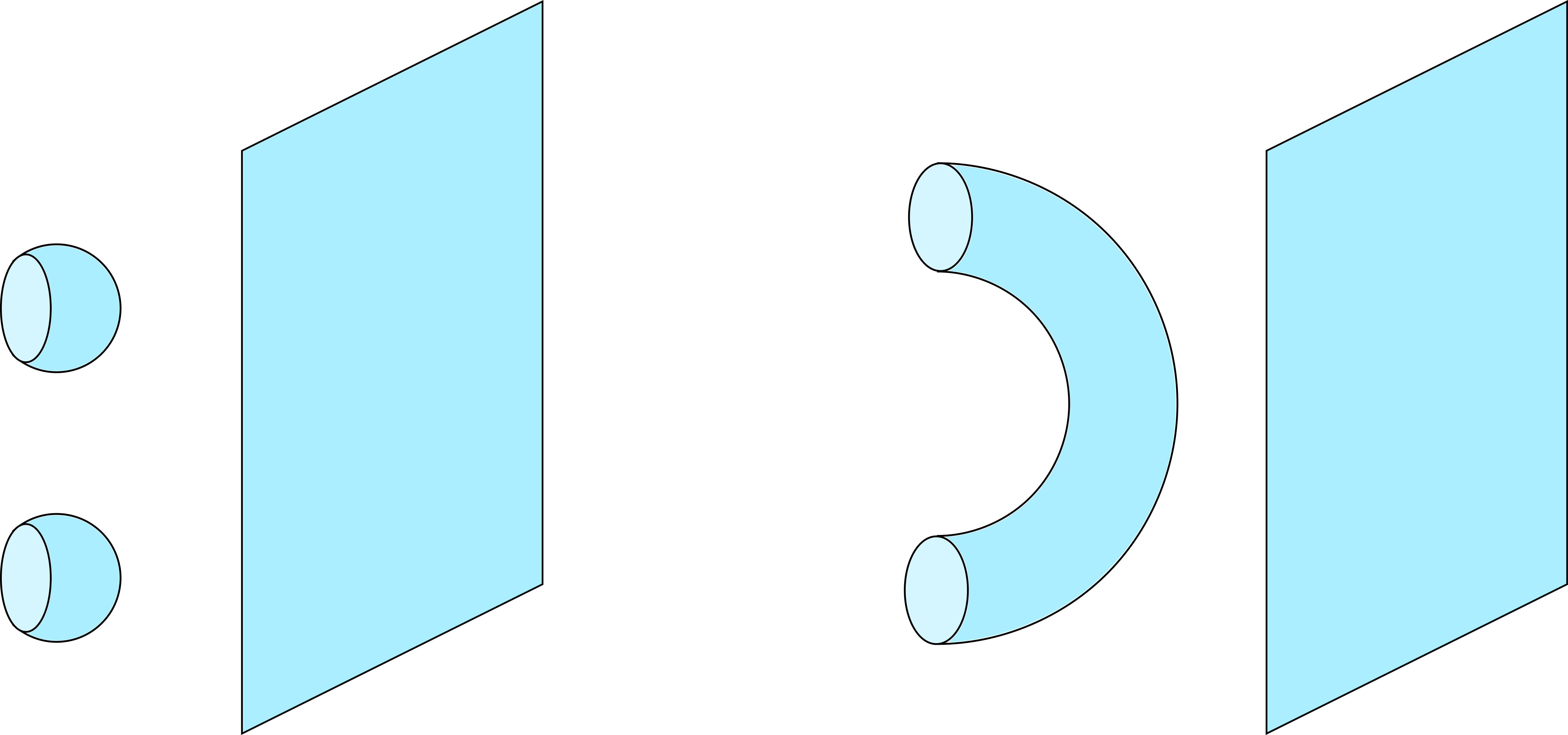
Refer to caption — Figure 1: Each $x$ denotes a circular boundary and the bracket $\langle\cdot\rangle$ denotes a bulk amplitude. The first two diagrams denote $\langle x^{2}\rangle\langle e^{\text{i}kx}\rangle$ and the last two diagrams denote the “connected” parts of the correlation function $2\langle x\rangle\langle xe^{\text{i}kx}\rangle_{c}+\langle x^{2}e^{\text{i}kx}\rangle_{c}$ .

We would like to get an estimation of the difference between any quantity $X^{n}$ and its ensemble average $\langle X^{n}\rangle$ , which requires a simple evaluation of $\langle x^{n}e^{ikx}\rangle$ . Motivated by the diagrams in Figure 1 and a similar proposal in Mukhametzhanov:2021hdi , we propose the following approximation

\displaystyle{\langle x^{2}e^{\text{i}kx}\rangle_{c}}\approx\langle xe^{\text{i}kx}\rangle_{\text{c}}\frac{1}{\langle e^{\text{i}kx}\rangle}\langle xe^{\text{i}kx}\rangle_{\text{c}}\,,

(10)

which has a diagrammatic interpretation as a recursive computation of configurations with a higher number of contractions to the spacetime brane from gluing the fundamental building blocks $\langle xe^{\text{i}kx}\rangle_{\text{c}}$ with the “propagator” $\langle e^{\text{i}kx}\rangle^{-1}$ .

Equivalently, this relation can be presented as

	$\displaystyle\frac{\langle x^{2}e^{\text{i}kx}\rangle}{\langle e^{\text{i}kx}\rangle}$	$\displaystyle\approx$	$\displaystyle\langle x^{2}\rangle-\langle x\rangle^{2}+\frac{\langle xe^{\text{i}kx}\rangle\langle xe^{\text{i}kx}\rangle}{\langle e^{\text{i}kx}\rangle\langle e^{\text{i}kx}\rangle}$		(11)
		$\displaystyle=$	$\displaystyle\langle x^{2}\rangle+2\langle x\rangle\frac{\langle xe^{\text{i}kx}\rangle_{\text{c}}}{\langle e^{\text{i}kx}\rangle}+\frac{\langle xe^{\text{i}kx}\rangle_{\text{c}}\langle xe^{\text{i}kx}\rangle_{\text{c}}}{\langle e^{\text{i}kx}\rangle\langle e^{\text{i}kx}\rangle}\ .$		(12)

Making use of the fact that the quantity $\langle e^{\text{i}kx}\rangle\equiv\varphi(k)$ is the characteristic function of the probability distribution whose inverse Fourier transformation is the PDF

\displaystyle\frac{1}{2\pi}\int\varphi(k)e^{-\text{i}kX}dk=P(X)\,,

(13)

the relation (10) is equivalent to

\displaystyle X^{2}

\displaystyle\approx

\displaystyle\langle X^{2}\rangle-\langle X\rangle^{2}+\Phi\,,\quad\Phi=\frac{1}{2\pi}\int dk\frac{e^{-\text{i}kX}}{P(X)}\langle e^{\text{i}kx}\rangle\left(\frac{\langle xe^{\text{i}kx}\rangle}{\langle e^{\text{i}kx}\rangle}\right)^{2}.

(14)

A more instructive form of this approximation is

\displaystyle X^{2}\approx\langle X^{2}\rangle+\tilde{\Phi}\,,\quad\tilde{\Phi}=\frac{1}{2\pi}\int dk\frac{e^{-\text{i}kX}}{P(X)}\langle e^{\text{i}kx}\rangle\left(\frac{\langle xe^{\text{i}kx}\rangle^{2}_{c}}{\langle e^{\text{i}kx}\rangle^{2}}+\frac{2\langle x\rangle\langle xe^{\text{i}kx}\rangle_{c}}{\langle e^{\text{i}kx}\rangle}\right)\,,

(15)

where $\langle\tilde{\Phi}\rangle=0$ . We will call the connected piece $\langle X^{2}\rangle_{c}\equiv\langle X^{2}\rangle-\langle X\rangle^{2}$ the “wormhole” contribution and $\Phi$ the “half-wormhole” contribution although it’s mean value is non-vanishing.

As a simple example, the Gaussian distribution $\mathcal{N}(\mu,t^{2}+\mu^{2})$ has the non-vanishing cumulants

\displaystyle c_{1}=\mu,\quad c_{2}=t^{2},

(16)

such that

\displaystyle\frac{\langle xe^{\text{i}kx}\rangle}{\langle e^{\text{i}kx}\rangle}=\mu+\text{i}kt^{2},\quad\left(\frac{\langle xe^{\text{i}kx}\rangle}{\langle e^{\text{i}kx}\rangle}\right)^{2}=\mu^{2}-k^{2}t^{4}+2\text{i}k\mu t^{2}.

(17)

Substituting the above into (14) gives

\displaystyle\Phi=X^{2}-t^{2},

(18)

which means that for Gaussian distribution the approximation (14) is actually exact. Clearly, this approximation cannot be exact for an arbitrarily general probability distribution. For example, for exponential distribution $\mathcal{E}(\lambda)$ the half-wormhole part is given by

\displaystyle\Phi=\frac{X^{2}}{2}\ ,\qquad x\geq 0\,,

(19)

and we quantify the error by its ratio to the variance of $X^{2}$

\displaystyle\text{Error}=X^{2}-\langle X^{2}\rangle+\langle X\rangle^{2}-\Phi\,,\qquad\rho=\frac{\langle\text{Error}^{2}\rangle}{\langle X^{4}\rangle}=\frac{5}{24}\ .

(20)

In fact, the error of the approximation (10) or (14) can be derived explicitly for any general distribution. Denoting the cumulants of the probability distribution as $c_{n}$ , namely

\displaystyle\log\langle e^{\text{i}kx}\rangle\equiv\log\varphi(k)=\sum_{n=0}^{\infty}c_{n}\frac{(ik)^{n}}{n!}\,,

(21)

we find¹¹1Notice that $\langle\cdot\rangle_{c}$ is not a linear functional, so we don’t expect similar relations for $\langle x^{n}e^{ikx}\rangle$ .

\displaystyle(-\text{i}\partial_{k})\log\langle e^{\text{i}kx}\rangle=\frac{\langle xe^{\text{i}kx}\rangle}{\langle e^{\text{i}kx}\rangle}=\frac{\langle xe^{\text{i}kx}\rangle_{c}}{\langle e^{\text{i}kx}\rangle}+\langle x\rangle=\sum_{n=0}^{\infty}c_{n+1}\frac{(\text{i}k)^{n}}{n!}\,,

(22)

which means

\displaystyle\frac{\langle xe^{\text{i}kx}\rangle_{c}}{\langle e^{\text{i}kx}\rangle}=\sum_{n=1}^{\infty}c_{n+1}\frac{(\text{i}k)^{n}}{n!}\ .

(23)

Similarly,

\displaystyle(-\text{i}\partial_{k})^{2}\log\langle e^{\text{i}kx}\rangle=\frac{\langle x^{2}e^{\text{i}kx}\rangle}{\langle e^{\text{i}kx}\rangle}-\frac{\langle xe^{\text{i}kx}\rangle\langle xe^{\text{i}kx}\rangle}{\langle e^{\text{i}kx}\rangle\langle e^{\text{i}kx}\rangle}=\sum_{n=0}^{\infty}c_{n+2}\frac{(\text{i}k)^{n}}{n!}\,,

(24)

which means

\displaystyle\frac{\langle x^{2}e^{\text{i}kx}\rangle_{c}}{\langle e^{\text{i}kx}\rangle}-\frac{\langle xe^{\text{i}kx}\rangle_{\text{c}}\langle xe^{\text{i}kx}\rangle_{\text{c}}}{\langle e^{\text{i}kx}\rangle\langle e^{\text{i}kx}\rangle}=\sum_{n=1}^{\infty}c_{n+2}\frac{(\text{i}k)^{n}}{n!}\ .

(25)

The approximation (10) is thus originated from neglecting all higher $c_{k}$ with $k>2$ .

This implies that indeed the approximation (10) or (14) is exact when the distribution is Gaussian, namely $c_{n}=0$ for $n>2$ .

Similarly we can consider the approximation of $X^{n}$ . We first derive the approximation of the connected correlators in the presence of spacetime brane. Taking the higher order derivative of the cumulant generating functions, for example when $n=3$ , we get

\displaystyle(-\text{i}\partial_{k})^{3}\log\langle e^{\text{i}kx}\rangle=\frac{\langle x^{3}e^{\text{i}kx}\rangle}{\langle e^{\text{i}kx}\rangle}-3\frac{\langle x^{2}e^{\text{i}kx}\rangle\langle xe^{\text{i}kx}\rangle}{\langle e^{\text{i}kx}\rangle\langle e^{\text{i}kx}\rangle}+2\left(\frac{\langle xe^{\text{i}kx}\rangle}{\langle e^{\text{i}kx}\rangle}\right)^{3}\ .

(26)

Separating out connected and disconnected parts, we get

\displaystyle(-\text{i}\partial_{k})^{3}\log\langle e^{\text{i}kx}\rangle=\frac{\langle x^{3}e^{\text{i}kx}\rangle_{c}}{\langle e^{\text{i}kx}\rangle}-3\frac{\langle x^{2}e^{\text{i}kx}\rangle_{c}\langle xe^{\text{i}kx}\rangle_{c}}{\langle e^{\text{i}kx}\rangle\langle e^{\text{i}kx}\rangle}+2\left(\frac{\langle xe^{\text{i}kx}\rangle_{c}}{\langle e^{\text{i}kx}\rangle}\right)^{3}+\langle x^{3}\rangle_{c}\,,

(27)

where

\displaystyle\langle x^{3}\rangle_{c}=\langle x^{3}\rangle-3\langle x^{2}\rangle\langle x\rangle+2\langle x\rangle^{3}\,,

(28)

is the connected correlator that equals to $c_{3}$ . Therefore we arrive at

\displaystyle\frac{\langle x^{3}e^{\text{i}kx}\rangle_{c}}{\langle e^{\text{i}kx}\rangle}-3\frac{\langle x^{2}e^{\text{i}kx}\rangle_{c}\langle xe^{\text{i}kx}\rangle_{c}}{\langle e^{\text{i}kx}\rangle\langle e^{\text{i}kx}\rangle}+2\left(\frac{\langle xe^{\text{i}kx}\rangle_{c}}{\langle e^{\text{i}kx}\rangle}\right)^{3}=\sum_{n=1}^{\infty}c_{n+3}\frac{(\text{i}k)^{n}}{n!}\ .

(29)

This means up to the third cumulant we have approximately

\displaystyle\frac{\langle x^{3}e^{\text{i}kx}\rangle_{c}}{\langle e^{\text{i}kx}\rangle}\approx 3\frac{\langle x^{2}e^{\text{i}kx}\rangle_{c}\langle xe^{\text{i}kx}\rangle_{c}}{\langle e^{\text{i}kx}\rangle\langle e^{\text{i}kx}\rangle}-2\left(\frac{\langle xe^{\text{i}kx}\rangle_{c}}{\langle e^{\text{i}kx}\rangle}\right)^{3}\,,

(30)

and the error of this approximation is due to neglecting all $c_{k}$ with $k>3$ . It is clear from this computation that the error of this approximation can be determined by (14). If the accuracy requirement is only up to the second moment, it up to quadratic fluctuations, we can use the approximation (10) again to get

\displaystyle\frac{\langle x^{3}e^{\text{i}kx}\rangle_{c}}{\langle e^{\text{i}kx}\rangle}\approx\left(\frac{\langle xe^{\text{i}kx}\rangle_{c}}{\langle e^{\text{i}kx}\rangle}\right)^{3}\ ,

(31)

which becomes exact when the distribution is Gaussian. In fact, we can derive similar relations by taking higher order derivatives in (26) to get relations among higher order $\langle x^{i}e^{\text{i}kx}\rangle_{c}$ ’s. If again we need accuracy up to quadratic order one can prove by induction

\displaystyle\frac{\langle x^{n}e^{\text{i}kx}\rangle_{c}}{\langle e^{\text{i}kx}\rangle}\approx\left(\frac{\langle xe^{\text{i}kx}\rangle_{c}}{\langle e^{\text{i}kx}\rangle}\right)^{n}\ .

(32)

We can then approximate the un-average $X^{3}$ to a required accuracy. In practice, we rewrite the definition of $X^{n}$ according to (2), then expand the $\langle x^{n}e^{\text{i}kx}\rangle$ in (2) in terms of the connected correlators $\langle x^{i}e^{\text{i}kx}\rangle_{c}$ according to e.g. (4)-(6). Then depending on the accuracy requirement, we use relations analogous to either (30) or (61), (32), to write down the approximation and the error of the final approximation is the composition of the errors the different approximations of $\langle x^{n}e^{ikx}\rangle$ . The general expression of the approximation of $X^{n}$ and the corresponding errors are complicated. But we will present some general procedures that work for any distribution once an accuracy goal is given.

2.1.1 Recursion relations for approximations to arbitrary accuracy

Define $\Phi_{n}=\frac{1}{2\pi}\int\frac{e^{\text{i}kX}}{P(X)}\langle e^{\text{i}kx}\rangle^{1-n}\langle xe^{\text{i}kx}\rangle^{n}$ , we have

\displaystyle X^{m}\Phi_{n}

\displaystyle=\frac{1}{2\pi}\int\frac{X^{m}e^{\text{i}kX}}{P(X)}\langle e^{\text{i}kx}\rangle^{1-n}\langle xe^{\text{i}kx}\rangle^{n}=\frac{1}{2\pi}\int\frac{e^{\text{i}kX}}{P(X)}\left(-i\partial_{k}\right)^{m}\left(\langle e^{\text{i}kx}\rangle^{1-n}\langle xe^{\text{i}kx}\rangle^{n}\right)\ .

(33)

Evaluating the derivative gives a result involving $\langle x^{i}e^{\text{i}kx}\rangle$ with $1\leq i\leq m+1$ . Rewriting them in terms of $\langle x^{i}e^{\text{i}kx}\rangle_{c}$ with the help of e.g. (4)-(6). Then use the approximation either (30) or (61), (32) according to the required accuracy. Then rewrite the $\langle x^{i}e^{\text{i}kx}\rangle_{c}$ in the approximated results back in terms of $\langle x^{i}e^{\text{i}kx}\rangle$ , and the result will be a relation among $\Phi_{i}$ with $1\leq i\leq m+1$ . Making use of the fact that $\Phi_{1}=X$ and recursively carrying out the above procedure to evaluate $X^{n-1}\Phi_{1}$ , we get the approximation of $X^{n}$ to the desired accuracy.

For example, if we require accuracy to the second order, we simply consider

\displaystyle X\Phi_{n}

\displaystyle=\frac{1}{2\pi}\int\frac{e^{\text{i}kX}}{P(X)}\langle e^{\text{i}kx}\rangle^{-n}\left(n\langle x^{2}e^{\text{i}kx}\rangle\langle xe^{\text{i}kx}\rangle^{n-1}\langle e^{\text{i}kx}\rangle+(1-n)\langle xe^{\text{i}kx}\rangle^{n+1}\right)\ .

(34)

Following the above procedure to rewrite $\langle x^{2}e^{\text{i}kx}\rangle$ , we arrive at

\displaystyle X\Phi_{n}=n\left(\langle x^{2}\rangle-\langle x\rangle^{2}\right)\Phi_{n-1}+\Phi_{n+1}\ .

(35)

For example, we can evaluate

\displaystyle X^{3}=X^{2}\Phi_{1}=3\left(\mu_{2}-\mu_{1}^{2}\right)\Phi_{1}+\Phi_{3}\,,

(36)

where we keep only accuracy up to the quadratic order, so $\mu_{3}$ does not appear independently; it is simply replaced by

\displaystyle\mu_{3}=3\mu_{1}\mu_{2}-2\mu_{1}^{3}\ .

(37)

2.1.2 Explicit relations for Gaussian approximation

If we only want Gaussian approximations of $X^{n}$ , we can get an explicit approximation formula. First let introduce some convenient notations

	$\displaystyle\phi_{n}=\frac{\langle x^{n}e^{\text{i}kx}\rangle}{\langle e^{\text{i}kx}\rangle},\quad\phi^{c}_{n}=\frac{\langle x^{n}e^{\text{i}kx}\rangle_{c}}{\langle e^{\text{i}kx}\rangle},$		(38)
	$\displaystyle\langle x^{n}\rangle=\mu_{n},\quad\langle x^{n}\rangle_{\text{cumulant}}=c_{n}.$		(39)

The cumulant $c_{m}$ can be expressed as a polynomial of moments

\displaystyle c_{m}=P_{m}(\mu_{m},\mu_{m-1},\dots,\mu_{1}).

(40)

Some examples are

\displaystyle c_{1}=\mu_{1},\quad c_{2}=\mu_{2}-\mu_{1}^{2},\quad c_{3}=\mu_{3}-3\mu_{1}\mu_{2}+2\mu_{1}^{3},\dots

(41)

Note that the coefficient of $\mu_{m}$ is 1. Of course the relations can be inverted

\displaystyle\mu_{m}=Q_{m}(c_{m},c_{m-1},\dots c_{1}).

(42)

Similar to (4),(5) and (6), $\phi_{n}$ can be decomposed as

\displaystyle\phi_{m}=\tilde{P}_{m}(\phi_{m}^{c},\dots,\phi_{0}^{c}),

(43)

for example

\displaystyle\phi_{1}=\phi_{1}^{c}+\mu_{1}\phi_{0}^{c},\quad\phi_{2}=\phi_{2}^{c}+2\mu_{1}\phi_{1}^{c}+\mu_{2},\dots.

(44)

Since $\log\langle e^{\text{i}kx}\rangle$ is the generating function of $c_{n}$ we have ²²2The simplest way to see this is to set $k=0$ , then it reduces to (40) and to notice that the coefficients of the polynomial $P_{m}$ do not depend on $k$ .

\displaystyle(-\text{i}\partial_{k})^{m}\log\langle e^{\text{i}kx}\rangle=P_{m}(\phi_{m},\phi_{m-1},\dots,\phi_{1})=\sum_{n=0}c_{n+m}\frac{(\text{i}k)^{n}}{n!}.

(45)

Using (43) and (42) the left-hand side can be expanded as a polynomial of $c_{i}$ with coefficients to be functions of $\phi_{i}^{c}$ :

\displaystyle P_{m}(\phi_{m},\phi_{m-1},\dots,\phi_{1})=P_{m}(\tilde{P}_{m}(\phi_{i}^{c}),\tilde{P}_{m-1}(\phi_{i}^{c}),\dots,\tilde{P}_{1}(\phi_{i}^{c}))\ .

(46)

For example

$\displaystyle P_{2}$	$\displaystyle=$	$\displaystyle\phi_{2}-\phi_{1}^{2}=\tilde{P}_{2}-2{\tilde{P}_{1}}^{2}$	(47)
	$\displaystyle=$	$\displaystyle\phi_{2}^{c}+2\mu_{1}\phi_{1}^{c}+\mu_{2}-{\phi_{1}^{c}}^{2}-\mu_{1}^{2}{\phi_{0}^{c}}^{2}-2\mu_{1}\phi_{1}^{c}\phi_{0}^{c}$	(48)
	$\displaystyle=$	$\displaystyle\phi_{2}^{c}-{\phi_{1}^{c}}^{2}+c_{1}(2\phi_{1}^{c}-2\phi_{1}^{c}\phi_{0}^{c})+c_{2}.$	(49)

Therefore we end up with

\displaystyle P_{m}=M_{m}+c_{1}M_{m-1}^{(1)}+(c_{1}^{2}M_{m-2}^{(1)}+c_{2}M_{m-2}^{(2)})+\dots+c_{m}=\sum_{n=0}c_{n+m}\frac{(\text{i}k)^{n}}{n!}\,,

(50)

where each $M_{i}^{(k)}$ is a function of the $\phi^{c}_{i}$ ’s. Since the subscript $i$ of $\phi^{c}_{i}$ and $M_{i}$ both indicate the power of $x$ , it is clear that

\displaystyle\sum_{a}i_{a}=m\,,\qquad\forall\left(\prod_{a}\phi_{i_{a}}^{c}\right)\in M_{m}\,,

(51)

where $\prod_{a}\phi_{i_{a}}^{c}$ is any term in $M_{m}$ . Notice that these relations are true for arbitrary $k$ , $m$ and distributions, then the non-trivial solution is only

\displaystyle\quad M_{n}^{(p)}=0\,,\qquad M_{m}=P_{m}(\phi^{c}_{m},\phi^{c}_{m-1},\dots,\phi^{c}_{1})=\sum_{n=1}c_{n+m}\frac{(\text{i}k)^{n}}{n!}\ .

(52)

The Gaussian approximation means $c_{m}=0$ for all $m>2$ . This requires

\displaystyle P_{m}(\phi^{c}_{m},\phi^{c}_{m-1},\dots,\phi^{c}_{1})\approx 0\,,\quad\forall m>1\ .

(53)

At $m=2$ this relation means

\displaystyle P_{2}(\phi^{c}_{2},\phi^{c}_{1})\approx 0\,,

(54)

which combines with (51) means $\phi^{c}_{2}=\alpha\left(\phi^{c}_{1}\right)^{2}$ and

\displaystyle P_{2}(\alpha\phi^{c}_{2},\phi^{c}_{1})=0\ .

(55)

To fix the normalization $\alpha$ , we notice that since the above relations (40) -(53), in particular the functional form of $P$ , are true for arbitrary distribution, we can choose the delta function distribution such that $c_{n}=0,\forall n\geq 2$ and $\mu_{m}=\mu_{1}^{m}$ , we can get the identity

\displaystyle P_{m}(\mu^{m},\mu^{m-1},\dots\mu)=0,\quad m\geq 2,

(56)

thus combining this with (55) we conclude $\alpha=1$ and

\displaystyle\phi^{c}_{2}\approx\left(\phi^{c}_{1}\right)^{2}\,,

(57)

where $\approx$ is due to the Gaussian approximation. This is nothing but the approximation (10). Iterating this procedure successively for different $m$ , we reach to

\displaystyle\phi_{m}^{c}\approx{(\phi_{1}^{c})}^{m}\,,

(58)

in the Gaussian approximation. Then we can approximate $X^{m}$ as

$\displaystyle X^{m}$	$\displaystyle=$	$\displaystyle\frac{1}{2\pi}\int\frac{e^{\text{i}kX}}{P(X)}\langle e^{\text{i}kx}\rangle\phi_{m}=\frac{1}{2\pi}\int\frac{e^{\text{i}kX}}{P(X)}\langle e^{\text{i}kx}\rangle\tilde{P}_{m}(\phi_{m}^{c},\dots,\phi_{1}^{c},1)$	(59)
	$\displaystyle\approx$	$\displaystyle\frac{1}{2\pi}\int\frac{e^{\text{i}kX}}{P(X)}\langle e^{\text{i}kx}\rangle\tilde{P}_{m}((\phi_{1}^{c})^{m},(\phi_{1}^{c})^{m-1},\dots,\phi_{1}^{c},1)$	(60)
	$\displaystyle=$	$\displaystyle\sum_{i=0}^{m}{m\choose i}\mu_{i}\Phi_{m-i}\,,$	(61)

where $\Phi_{i}=\frac{1}{2\pi}\int\text{d}k\frac{e^{\text{i}kX}}{P(X)}\langle e^{\text{i}kx}\rangle(\phi_{1}^{c})^{i}$ , and it may be understood as generalized wormholes which we will report somewhere else.

It is easy to check that the result (61) agrees with (36) once the relation (37) is used.

2.2 Models with multiple independent identical random variables

In statistical models with a single random variable, the various moments are all observables that we can compute. On the other hand, we would like to consider other interesting observables. We therefore proceed to consider operators in statistical models with multiple independent identical random variables.

One class of operators in these models is the light operators that are simply linear combinations of the random variables $X_{i}$ . We conjecture that if $Y(X_{i})$ is some function of a large number $N$ independent random variables $X_{i}$ such that $Y$ is approximately Gaussian, then the approximation

	$\displaystyle Y^{2}\approx\langle Y^{2}\rangle-\langle Y\rangle^{2}+\Phi,$		(62)
	$\displaystyle\Phi(X)=\frac{1}{(2\pi)^{N}}\int\prod_{i}\left(dk_{i}\frac{e^{-\text{i}k_{i}X_{i}}}{P(X_{i})}\right)\langle e^{\text{i}\sum_{i}k_{i}x_{i}}\rangle\left(\frac{\langle Y(x)e^{\text{i}\sum_{i}k_{i}x_{i}}\rangle}{\langle e^{\text{i}\sum_{i}k_{i}x_{i}}\rangle}\right)^{2}.$		(63)

is good in the sense that

\displaystyle\rho\equiv\frac{\langle\text{Error}^{2}\rangle}{\langle Y^{2}\rangle^{2}}\,,

(64)

is suppressed by $1/N$ .

Like (15) we can rewrite it into

	$\displaystyle Y^{2}\approx\langle Y^{2}\rangle+\tilde{\Phi},$		(65)
	$\displaystyle\tilde{\Phi}(X)=\frac{1}{(2\pi)^{N}}\int\prod_{i}\left(dk_{i}\frac{e^{-\text{i}k_{i}X_{i}}}{P(X_{i})}\right)\langle e^{\text{i}\sum_{i}k_{i}x_{i}}\rangle\left(\frac{\langle Y(x)e^{\text{i}\sum_{i}k_{i}x_{i}}\rangle_{c}^{2}}{\langle e^{\text{i}\sum_{i}k_{i}x_{i}}\rangle^{2}}+\frac{2\langle Y\rangle\langle Y(x)e^{\text{i}\sum_{i}k_{i}x_{i}}\rangle_{c}}{\langle e^{\text{i}\sum_{i}k_{i}x_{i}}\rangle}\right).$		(66)

2.2.1 Simple observables

The fundamental logic in this section is that by the central limit theorem (CLT), summing over a large number of i.i.d random variables gives a random variable that approximately obey a Gaussian distribution. Explicitly, if $X_{i}$ is from a normal distribution ${\cal N}(\mu,\sigma^{2})$ , then the mean of $N$ such i.i.d’s

\displaystyle\tilde{Y}=\frac{1}{N}\sum_{i=1}^{N}X_{i}\,,

(67)

is approximately a Gaussian random variable from ${\cal N}(\mu,\sigma^{2}/N)$ when $N$ is large enough.

In this paper, it turns out that it is more convenient to define

\displaystyle Y=\sum_{i=1}^{N}X_{i}\,,

(68)

so that the connection to the SYK model is more transparent. Then $Y$ is a Gaussian random variable with probability distribution ${\cal N}(N\mu,N\sigma^{2})$ when $N$ is large. In particular, we expect

\displaystyle\langle Y^{4}\rangle\approx 3\langle Y^{2}\rangle^{2}-2\langle Y\rangle^{4}\,,\quad\langle Y^{2}\rangle\approx N\left(\langle X^{2}\rangle-\langle X\rangle^{2}\right)+N^{2}\langle X\rangle^{2}\,,\quad\langle Y\rangle\approx N\langle X\rangle\ .

(69)

They can be checked by a direct calculation

	$\displaystyle\langle Y^{2}\rangle=N\langle X^{2}\rangle+N(N-1)\langle X\rangle^{2},$		(70)
	$\displaystyle\langle Y^{4}\rangle=N\langle X^{4}\rangle+N(N-1)\left(4\langle X^{3}\rangle\langle X\rangle+3\langle X^{2}\rangle^{2}\right)$
	$\displaystyle\quad+6N(N-1)(N-2)\langle X^{2}\rangle\langle X\rangle^{2}+N(N-1)(N-2)(N-3)\langle X\rangle^{4}\ .$		(71)

Because all the $X_{i}$ are independent so that it is straightforward to obtain

\displaystyle\frac{\langle Ye^{\text{i}k_{i}x_{i}}\rangle}{\langle e^{\text{i}k_{i}x_{i}}\rangle}=\sum_{i}\frac{\langle x_{i}e^{\text{i}k_{i}x_{i}}\rangle}{\langle e^{\text{i}k_{i}x_{i}}\rangle}\equiv\sum_{i}k_{i}[1].

(72)

Next we can rewrite the square of (72) into the diagonal terms and off-diagonal terms

\displaystyle\left(\frac{\langle Ye^{\text{i}k_{i}x_{i}}\rangle}{\langle e^{\text{i}k_{i}x_{i}}\rangle}\right)^{2}=\sum_{i}k_{i}[1]^{2}+\sum_{i\neq j}k_{i}[1]k_{j}[1].

(73)

To compute the off-diagonal contributions to the half-wormhole, we observe that

	$\displaystyle\frac{1}{(2\pi)^{N}}\int\prod_{i}\left(dk_{i}\frac{e^{-\text{i}k_{i}X_{i}}}{P(X_{i})}\right)\langle e^{\text{i}\sum_{i}k_{i}x_{i}}\rangle k_{i}[1]k_{j}[1]$		(74)
	$\displaystyle=\frac{1}{(2\pi)^{2}}\int dk_{i}dk_{j}\frac{e^{-\text{i}k_{i}X_{i}-\text{i}k_{j}X_{j}}}{P(X_{i})P(X_{j})}\langle x_{i}e^{\text{i}k_{i}x_{i}}\rangle\langle x_{j}e^{\text{i}k_{j}x_{j}}\rangle=X_{i}X_{j}\ .$		(75)

In terms of $\widehat{k_{i}[n]^{m}}$ which are defined in (585) the half-wormhole can be written as

\displaystyle\Phi=\sum_{i}\widehat{k_{i}[1]^{2}}+\sum_{i\neq j}X_{i}X_{j},

(76)

and the error is given by

	Error	$\displaystyle=\sum_{i}\left(X_{i}^{2}-\widehat{k_{i}[1]^{2}}-t^{2}\right),\quad t^{2}=\langle X_{i}^{2}\rangle-\langle X_{i}\rangle^{2}\,,$		(77)
	$\displaystyle\langle\text{Error}^{2}\rangle$	$\displaystyle=\sum_{i,j}\langle(X_{i}^{2}-\widehat{k_{i}[1]^{2}})(X_{j}^{2}-\widehat{k_{j}[1]^{2}})\rangle+N^{2}t^{4}-2Nt^{2}\sum_{i}(X_{i}^{2}-\widehat{k_{i}[1]^{2}})\ .$		(78)

Recalling that $\langle Y^{2}\rangle\sim Nt^{2}$ so to prove the conjecture (62) we need to show that the ${\cal O}(N^{2})$ term in (78) vanish. A direct calculation gives

	$\displaystyle\langle\widehat{k_{i}[1]^{2}}\rangle_{X_{i}}$	$\displaystyle=$	$\displaystyle\int dX_{i}P(X_{i})k_{i}[1]^{2}\langle e^{\text{i}k_{i}x_{i}}\rangle_{x_{i}}\frac{e^{-\text{i}k_{i}X_{i}}}{P(X_{i})}dk_{i}$		(79)
		$\displaystyle=$	$\displaystyle\int dk_{i}\delta(-k_{i})\langle e^{\text{i}k_{i}x_{i}}\rangle_{x_{i}}k_{i}[1]^{2}=\langle X_{i}\rangle^{2}\ .$		(80)

This means

\displaystyle\langle(X_{i}^{2}-\widehat{k_{i}[1]^{2}}\rangle=\langle X^{2}_{i}\rangle-\langle X_{i}\rangle^{2}=t^{2}\ .\quad\Leftrightarrow\quad\langle\widehat{k_{i}[1]^{2}}\rangle_{X_{i}}\approx\langle X_{i}\rangle^{2}\ .

(81)

In particular, a consequence of this relation is that although all the 3 terms in (78) are of order ${\cal O}(N^{2})$ , the sum of them cancelled exactly since (81) does not depend on $i$ . This then shows that $\langle\text{Error}^{2}\rangle\ll\langle Y^{2}\rangle$ and hence the approximation (62) is valid.

We can derive this result in a more illuminating fashion. First using (23) $k_{i}[1]$ can be expressed as

\displaystyle k_{i}[1]=\sum_{n=0}\frac{(-\text{i}k)^{n}}{n!}c_{n+1}.

(82)

Then using the fact that the inverse Fourier transformation of the characteristic function is the PDF we find

	$\displaystyle\langle\widehat{k_{i}[1]^{2}}\rangle_{X_{i}}=\int dX_{i}P(X_{i})\sum_{n,m=0}\frac{c_{n+1}c_{m+1}}{n!m!}(-\text{i}k_{i})^{n+m}\langle e^{\text{i}k_{i}x_{i}}\rangle_{x_{i}}\frac{e^{-\text{i}k_{i}X_{i}}}{P(X_{i})}dk_{i}$		(83)
	$\displaystyle\quad=\int dX_{i}\sum_{n,m=0}\frac{c_{n+1}c_{m+1}}{n!m!}(\partial_{X_{i}})^{n+m}P(X_{i})=c_{1}^{2}=\langle X_{i}\rangle^{2}\ .$		(84)

2.2.2 Power-sum observables

In this section, we consider another class of more general observables

\displaystyle Y=\sum_{i}f(X_{i}),\quad Y^{2}=\sum_{i,j}f(X_{i})f(X_{j}),

(85)

where $X_{i}$ are still independent identical random variables with PDF $P_{X_{i}}$ and $f$ is some smooth function so that $f(X_{i})$ are also independent and identical random variables with a new PDF $P_{f}$ :

\displaystyle\int dXF[f(X)]P_{X}=\int dfF(f)P_{f}.

(86)

The CLT is still valid but the proposal may not because naively it depends on the function $f$ . By smooth function we mean $f(X_{i})$ is not singular anywhere such that it can be Taylor expanded

\displaystyle f(X_{i})=\sum_{n}a_{n}X_{i}^{n}\,,

(87)

whose expansion coefficients satisfy

\displaystyle a_{n}\approx 0\,,\qquad\forall n>n_{0}\,,\quad n_{0}\ll N\ .

(88)

Accordingly (72) and (73) become

	$\displaystyle\frac{\langle Ye^{\text{i}k_{i}x_{i}}\rangle}{\langle e^{\text{i}k_{i}x_{i}}\rangle}=\sum_{i}\sum_{n}a_{n}k_{i}[n].$		(89)
	$\displaystyle\left(\frac{\langle Ye^{\text{i}k_{i}x_{i}}\rangle}{\langle e^{\text{i}k_{i}x_{i}}\rangle}\right)^{2}=\sum_{i,j}\left(\sum_{n}a_{n}k_{i}[n]\sum_{m}a_{m}k_{j}[m]\right).$		(90)

So the error is given by

Error	$\displaystyle=\sum_{i}\left(f^{2}(X_{i})-t^{2}-\sum_{n,m}a_{n}a_{m}\widehat{k_{i}[n]k_{i}[m]}\right)\,,$	(91)
$\displaystyle\langle\text{Error}^{2}\rangle$	$\displaystyle=\langle\sum_{i,j}(f^{2}(X_{i})-\sum_{n,m}a_{n}a_{m}\widehat{k_{i}[n]k_{i}[m]})(f^{2}(X_{j})-\sum_{n,m}a_{n}a_{m}\widehat{k_{j}[n]k_{j}[m]})\rangle$
	$\displaystyle\quad+N^{2}t^{4}-2Nt^{2}\sum_{i}(f^{2}(X_{i})-\sum_{n,m}a_{n}a_{m}\widehat{k_{i}[n]k_{i}[m]})\,,$	(92)

where $t^{2}=\langle f^{2}(X_{i})\rangle-\langle f(X_{i})\rangle^{2}$ . Similar to the calculation of (80), one can find

\displaystyle\langle\sum_{n,m}a_{n}a_{m}\widehat{k_{i}[n]k_{i}[m]}\rangle=\langle f(X_{i})\rangle^{2},

(93)

which means the leading order terms, ie of order $N^{2}$ , in (92) is

\displaystyle 2\left(\langle(f^{2}(X_{j})-\sum_{n,m}a_{n}a_{m}\widehat{k_{j}[n]k_{j}[m]})\rangle^{2}-t^{4}\right)N^{2}=0\,,

(94)

As a result, the error is small and indeed the approximation (62) is reasonable in this case too. We also show some explicit examples in the Appendix (B). More generally, following the same procedure one can show that the half wormhole proposal is correct for the following family of functions

\displaystyle Y_{k}=\sum_{i}^{N}\left(f(X_{i_{1}},X_{i_{2}},\dots,X_{i_{k}})\right),

(95)

where $X_{i_{p}}$ are independent and identical random variables.

2.2.3 Product observables

Previously the function $Y$ we considered are a summation of (polynomials of) independent random variables. The proposal works very well for all the probability distributions. However in the original construction of half wormhole introduced in Saad:2021rcu , the function $Y$ is a determinant observables which are “heavy” in the traditional field theory language

\displaystyle Y=\text{PF}(J)=\sum^{\prime}_{A_{1}<A_{2}<\dots<A_{p}}\text{sgn}(A){J}_{A_{1}}{J}_{A_{2}}\dots J_{A_{p}},

(96)

where the function $\text{PF}(J)$ is called the hyperpfaffian Barvinok which is a tensorial generalization of pfaffian and $J_{A_{i}}$ are random variables. To mimic this construction let us consider a similar model:

\displaystyle Y=\sum_{i_{1}\neq i_{2}\neq\dots\neq i_{q}}^{N}X_{i_{1}}X_{i_{2}}\dots X_{i_{q}}.

(97)

$\bullet$ $q=2$ Gaussian distribution
The simplest case is $q=2$ :

	$\displaystyle Y=\sum_{i\neq j}X_{i}X_{j},$		(98)
	$\displaystyle Y^{2}=\sum_{i\neq j\neq p\neq q}X_{i}X_{j}X_{p}X_{q}+4\sum_{i\neq j\neq p}X_{i}^{2}X_{j}X_{p}+2\sum_{i\neq j}X_{i}^{2}X_{j}^{2}\ .$		(99)

It is straightforward to get

	$\displaystyle\langle Y^{2}\rangle=N(N-1)\left(2t^{4}+4(N-1)\mu^{2}t^{2}+N(N-1)\mu^{4}\right),$		(100)
	$\displaystyle\langle X_{i}\rangle=\mu,\quad\langle X^{2}\rangle-\langle X\rangle^{2}=t^{2}.$		(101)

So in general $\langle Y^{2}\rangle$ will scale as $N^{4}$ if $\mu\neq 0$ , while if $\mu=0$ it scales as $N^{2}$ .

One example of the $\mu=0$ case is the Gaussian distribution $\mathcal{N}(\mu=0,t^{2})$ . We then verifies

\displaystyle\langle Y\rangle=0,\quad\langle Y^{2}\rangle=2t^{4}N(N-1)

(102)

and

\displaystyle\Phi=\sum_{i\neq j\neq p\neq q}X_{i}X_{j}X_{p}X_{q}+4\sum_{i\neq j\neq p}(X_{i}^{2}-t^{2})X_{j}X_{p}+2\sum_{i\neq j}(X_{i}^{2}-t^{2})(X_{j}^{2}-t^{2})\ .

(103)

Therefore we obtain

	$\displaystyle\text{Error}=-2t^{4}N(N-1)+4t^{2}(N-2)\sum_{i\neq j}X_{i}X_{j}+4(N-1)t^{2}\sum_{i}X_{i}^{2}-2t^{4}N(N-1),$
	$\displaystyle\langle(\text{Error}/4)^{2}\rangle=(2+1+1-2)N^{4}t^{8}+\#N^{3}+\dots$		(104)

the leading term does not vanish so the approximation

\displaystyle Y^{2}\approx\langle Y^{2}\rangle-\langle Y\rangle^{2}+\Phi\,,

(105)

is not good.

However, for more general Gaussian distributions $\mathcal{N}(\mu,t^{2})$ similar calculation gives

\displaystyle\langle Y\rangle=N(N-1)\mu^{2},\quad\langle Y^{2}\rangle-\langle Y\rangle^{2}\equiv\tilde{t}^{2}=2t^{2}N(N-1)(t^{2}+2(N-1)\mu^{2}),

(106)

and

\displaystyle\text{Error}=-\tilde{t}^{2}+4t^{2}(N-2)\sum_{i\neq j}X_{i}X_{j}+4(N-1)t^{2}\sum_{i}X_{i}^{2}-2t^{4}N(N-1),

(107)

now we find that

\displaystyle\langle\text{Error}^{2}\rangle=32(3t^{2}\mu^{2}+\mu^{4})N^{5}+32(t^{4}-12t^{2}\mu^{2}-4\mu^{4})N^{4}+\dots

(108)

and

\displaystyle\frac{\langle\text{Error}^{2}\rangle}{\langle Y^{2}\rangle^{2}}=\frac{2(\mu^{4}+3t^{2}\mu^{2}-3t^{4})}{(2t^{4}-4t^{2}\mu^{2})^{2}N}+\dots.

(109)

Notice that the error is always small, even when $\mu\rightarrow 0$ , and the proposal is valid. This is because when $\mu\neq 0$ , the moments of $Y$ behave as

\displaystyle\langle Y\rangle\approx N^{2}\mu,\quad\langle Y^{2}\rangle\approx N^{4}\mu^{2},\quad\langle Y^{4}\rangle\approx N^{8}\mu^{4},

(110)

as expected from (69). It is thus clear that the $\mu\to 0$ limit is not smooth.

It seems $\mu\neq 0$ is fundamentally better than the $\mu=0$ case in the sense that the approximation (62) is good. But as we will discuss shortly in section 2.3.1 this is not the case and the crucial point is that it is more appropriate to compare the error with the connected contributions and left out the disconnected contributions.

$\bullet$ General $q$
Next we consider general distributions. We show some details of the computation for exponential distribution and Poisson distribution in the Appendix (C). Here we only give a more abstract derivation. In terms of (585) the half wormhole (63) can be written as

	$\displaystyle\Phi$	$\displaystyle=$	$\displaystyle\sum_{i\neq j\neq p\neq q}\widehat{k_{i}[1]}\widehat{k_{j}[1]}\widehat{k_{p}[1]}\widehat{k_{q}[1]}+4\sum_{i\neq j\neq p}\widehat{k_{i}[1]^{2}}\widehat{k_{j}[1]}\widehat{k_{p}[1]}+2\sum_{i\neq j}\widehat{k_{i}[1]^{2}}\widehat{k_{j}[1]^{2}}$		(111)
		$\displaystyle=$	$\displaystyle\sum_{i\neq j\neq p\neq q}X_{i}X_{j}X_{p}X_{q}+4\sum_{i\neq j\neq p}\widehat{k_{i}[1]^{2}}X_{j}X_{p}+2\sum_{i\neq j}\widehat{k_{i}[1]^{2}}\widehat{k_{j}[1]^{2}}.$		(112)

Therefore the error of the proposal is

\displaystyle\text{Error}=4\sum_{i\neq j\neq q}(X_{i}^{2}-\widehat{k_{i}[1]^{2}})X_{j}X_{p}+2\sum_{i\neq j}(X_{i}^{2}X_{j}^{2}-\widehat{k_{i}[1]^{2}}\widehat{k_{j}[1]^{2}})-\tilde{t}^{2}.

(113)

The maximal power of $N$ in $\langle\text{Error}^{2}\rangle$ will be $6$ .

When $\mu\neq 0$ , $\langle Y^{2}\rangle^{2}\sim N^{8}$ . So in this case the error is small and the approximation is good.

When $\mu=0$ , $\langle Y^{2}\rangle^{2}\sim N^{4}$ . The terms of $N^{4}$ in $\langle\text{Error}^{2}\rangle$ come from

$\displaystyle\langle\text{Error}^{2}\rangle$	$\displaystyle=$	$\displaystyle\langle\sum_{i\neq j\neq p\neq q}\{16\times 2(X_{i}^{2}-\widehat{k_{i}[1]^{2}})(X_{j}^{2}-\widehat{k_{j}[1]^{2}})X_{p}^{2}X_{q}^{2}$	(114)
	$\displaystyle+$	$\displaystyle 4(X_{i}^{2}X_{j}^{2}-\widehat{k_{i}[1]^{2}}\widehat{k_{j}[1]^{2}})(X_{p}^{2}X_{q}^{2}-\widehat{k_{p}[1]^{2}}\widehat{k_{q}[1]^{2}})\}$
	$\displaystyle+$	$\displaystyle 4t^{16}N^{4}-8t^{4}N^{2}\sum_{i\neq j}(X_{i}^{2}X_{j}^{2}-\widehat{k_{i}[1]^{2}}\widehat{k_{j}[1]^{2}})\rangle+\dots$
	$\displaystyle=$	$\displaystyle N^{4}t^{16}\left(32+4+4-8\right)+\#N^{3}\dots=32N^{4}t^{16}+\#N^{3}\dots$	(115)

which is not vanishing so the error is large and we cannot approximate $Y^{2}$ by $\langle Y^{2}\rangle+\Phi$ probably for the same reason as the $q=2$ case. One could ask that when $\langle X_{i}^{2}-\widehat{k_{i}[1]^{2}}\rangle=0$ , the approximation might be fine, but it requires $t^{2}=0$ which we do not consider at the moment.

$\bullet$ General distributions

Now we consider the general case (97):

	$\displaystyle Y=\sum_{i_{1}\neq i_{2}\neq\dots\neq i_{q}}^{N}X_{i_{1}}X_{i_{2}}\dots X_{i_{q}},$		(116)
	$\displaystyle Y^{2}=\sum_{k=0}^{q}\frac{(q!/(q-k)!)^{2}}{k!}\sum_{j_{1}\neq j_{2}\dots j_{k}\neq i_{1}\dots\neq i_{2q-2k}}X_{j_{1}}^{2}\dots X_{j_{k}}^{2}X_{i_{1}}\dots X_{i_{2q-2k}}.$		(117)

If $N\gg q$ then the average $\langle Y^{2}\rangle$ will have the following scaling behavior in the large $N$ limit

\displaystyle\langle Y^{2}\rangle\sim\begin{cases}N^{2q}\mu^{2q}&\quad\mu\neq 0\\ N^{q}q!t^{2q}&\quad\mu=0\end{cases}

(118)

Similar to (112), one can find that the half wormhole contribution $\Phi$ can be written as

\displaystyle\Phi

\displaystyle=

\displaystyle\sum_{k=0}^{q}\frac{(q!/(q-k)!)^{2}}{k!}\sum_{j_{1}\neq j_{2}\dots j_{k}\neq i_{1}\dots\neq i_{2q-2k}}\widehat{k_{j_{1}}[1]^{2}}\dots\widehat{k_{j_{k}}[1]^{2}}X_{i_{1}}\dots X_{i_{2q-2k}},

(119)

so that the error is

	Error	$\displaystyle=$	$\displaystyle\sum_{k=1}^{q}\frac{(q!/(q-k)!)^{2}}{k!}\sum_{\begin{subarray}{c}j_{1}\neq j_{2}\dots j_{k}\neq\\ i_{1}\dots\neq i_{2q-2k}\end{subarray}}(X_{j_{1}}^{2}\dots X_{j_{k}}^{2}-\widehat{k_{j_{1}}[1]^{2}}\dots\widehat{k_{j_{k}}[1]^{2}})X_{i_{1}}\dots X_{i_{2q-2k}}$		(120)
		$\displaystyle-$	$\displaystyle\langle Y^{2}\rangle+\langle Y\rangle^{2}.$		(120)

When $\mu\neq 0$ , the leading contribution to $\langle\text{Error}^{2}\rangle$ scales as $N^{2q-2}$ so the approximation (62) is correct.

However when $\mu=0$ , the leading contributions to $\langle\text{Error}^{2}\rangle$ are

$\displaystyle\langle\text{Error}^{2}\rangle$	$\displaystyle=E_{1}+E_{2}+\#N^{2q-1},$	(121)
$\displaystyle E_{1}$	$\displaystyle=\langle\sum_{k=1}^{q}\left(\frac{(q!/(q-k)!)^{2}}{k!}\right)^{2}(2q-2k)!$	(122)
	$\displaystyle\quad\times\sum_{\begin{subarray}{c}j_{1}\neq j_{2}\dots\neq j_{2k}\\ \neq i_{1}\neq\dots\neq i_{2q-2k}\end{subarray}}(X_{j_{1}}^{2}-\widehat{k_{j_{1}}[1]^{2}})\dots(X_{j_{k}}^{2}-\widehat{k_{j_{2k}}[1]^{2}})X_{i_{1}}^{2}\dots X_{i_{2q-2k}}^{2}\rangle$
	$\displaystyle=N^{2q}t^{4q}(2q)!\left(\,{}_{3}F_{2}\left(-q,-q,-q;1,\frac{1}{2}-q;\frac{1}{4}\right)-1\right)\neq 0,$	(123)
$\displaystyle E_{2}$	$\displaystyle=\langle\left(q!\sum_{i_{1}\neq i_{2}\neq\dots\neq i_{q}}^{N}(X_{i_{1}}^{2}\dots X_{i_{q}}^{2}-\widehat{k_{i_{1}}[1]^{2}}\dots\widehat{k_{i_{q}}[1]^{2}})-q!N^{q}\right)^{2}\rangle=0\ .$	(124)

So the error is large as in the previous case (115) and the approximation (62) is not good.

In our toy model (97) we did not include the “diagonal” terms while from our analysis above we have shown in the large $N$ limit it is the “off-diagonal” term that dominates. So our conclusions for (97) are also valid for the following general function

\displaystyle Y=\sum_{i_{1},i_{2},\dots,i_{q}=1}^{N}X_{i_{1}}X_{i_{2}}\dots X_{i_{q}}..

(125)

As a simple demonstration, let us still consider the simplest case with $q=2$ :

	$\displaystyle Y=\sum_{i,j}X_{i}X_{j},$		(126)
	$\displaystyle Y^{2}=\sum_{i}X_{i}^{4}+4\sum_{i\neq j}X_{i}^{3}X_{j}+3\sum_{i\neq j}X_{i}^{2}X_{j}^{2}$
	$\displaystyle\qquad+6\sum_{i\neq j\neq k}X_{i}X_{j}X_{k}^{2}+\sum_{i\neq j\neq m\neq n}X_{i}X_{j}X_{m}X_{n}.$		(127)

Comparing

$\displaystyle\langle Y^{2}\rangle=$	$\displaystyle N^{4}\kappa_{1}^{4}+4N^{2}\kappa_{3}\kappa_{1}+3N^{2}\kappa_{2}^{2}+6N^{3}\kappa_{2}\kappa_{1}^{2}+N\kappa_{4},$	(131)
	$\displaystyle\kappa_{1}=\langle X\rangle=\mu,\quad\kappa_{2}=\langle X^{2}\rangle-\langle X\rangle^{2}=t^{2},$
	$\displaystyle\kappa_{3}=\langle X^{3}\rangle-3\langle X\rangle\langle X^{2}\rangle+2\langle X^{3}\rangle,$
	$\displaystyle\kappa_{4}=\langle X^{4}\rangle-3\langle X^{2}\rangle^{2}-4\langle X\rangle\langle X^{3}\rangle+12\langle X\rangle^{2}\langle X^{2}\rangle-6\langle X\rangle^{4},$

with (100) one find that if $t\neq 0$ , the scaling behavior of $\langle Y^{2}\rangle$ is same as before. The half wormhole contribution $\Phi$ can be work out similarly:

	$\displaystyle\Phi$	$\displaystyle=$	$\displaystyle\sum_{i}\widehat{k_{i}[2]^{2}}+\sum_{i\neq j}\widehat{k_{i}[2]}\widehat{k_{j}[2]}+\sum_{i\neq j\neq m\neq n}X_{i}X_{j}X_{m}X_{n}+4\sum_{i\neq j\neq m}\widehat{k_{i}[1]^{2}}X_{j}X_{m}$		(132)
		$\displaystyle+$	$\displaystyle 2\sum_{i\neq j}\widehat{k_{i}[1]^{2}}\widehat{k_{j}[1]^{2}}+2\sum_{i\neq j\neq k}\widehat{k_{i}[2]}X_{j}X_{k}+4\sum_{i\neq j}\widehat{k_{i}[2]k_{i}[1]}X_{j}$		(132)

Then the error is given by

Error	$\displaystyle=$	$\displaystyle 4\sum_{i\neq j\neq k}(X_{i}^{2}-\widehat{k_{i}[1]^{2}})X_{j}X_{k}+2\sum_{i\neq j\neq k}(X_{i}^{2}-\widehat{k_{i}[2]})X_{j}X_{k}+2\sum_{i\neq j}(X_{i}^{2}X_{j}^{2}-\widehat{k_{i}[1]^{2}}\widehat{k_{j}[1]^{2}})$	(133)
	$\displaystyle+$	$\displaystyle\sum_{i\neq j}(X_{i}^{2}X_{j}^{2}-\widehat{k_{i}[2]}\widehat{k_{j}[2]})+4\sum_{i\neq j}(X_{i}^{3}-\widehat{k_{i}[2]k_{i}[1]})X_{j}+\sum_{i}(X_{i}^{4}-\widehat{k_{i}[2]^{2}})\rangle-\tilde{t}^{2}.$
	$\displaystyle=$	$\displaystyle 4\sum_{i\neq j\neq k}(X_{i}^{2}-\widehat{k_{i}[1]^{2}})X_{j}X_{k}+2\sum_{i\neq j}(X_{i}^{2}X_{j}^{2}-\widehat{k_{i}[1]^{2}}\widehat{k_{j}[1]^{2}})$
	$\displaystyle+$	$\displaystyle 4\sum_{i\neq j}(X_{i}^{3}-\widehat{k_{i}[2]k_{i}[1]})X_{j}+\sum_{i}(X_{i}^{4}-\widehat{k_{i}[2]^{2}})\rangle-\tilde{t}^{2},$

where we have used the identity

\displaystyle\widehat{k[2]}=\int\text{d}k\frac{e^{-\text{i}kX}}{P(X)}\langle x^{2}e^{\text{i}kx}\rangle=X^{2}.

(134)

Comparing with (113), there are two extra terms in (133), but they will never contribute³³3If $\mu\neq 0$ they maximally contribute to $N^{5}$ and when $\mu=0$ they maximally contribute to $N^{3}$ . to the leading power of $N$ when $t\neq 0$ . So again it seems the approximation (62) is good when $\mu\neq 0$ but not good when $\mu=0$ . We will explain in the next section how to understand these results and modify the proposal (62).

2.3 Large- $N$ constraints and half-wormhole approximation

In the previous sections we consider a few different examples. To summarize, the half-wormhole conjecture (62) and (63) is valid for a large families of statistical models. However, for some examples discussed in section 2.2.3 this approximation is not good.

2.3.1 Why and how to modify the approximation proposal

The failed examples indicate that the proposed $\Phi$ does not capture all semi-classical components in the observable $Y^{2}$ to be approximated.

As discussed previously, the approximation (62) should come from the approximation (10). The relation (10) indeed fails for the case where the approximation (62) is not good in section (2.2.3). To see this explicitly, we consider the simplest example (98) where

\displaystyle Y^{2}

\displaystyle=\sum_{i\neq j\neq p\neq q}X_{i}X_{j}X_{p}X_{q}+4\sum_{i\neq p\neq q}X_{i}^{2}X_{p}X_{q}+2\sum_{i\neq j}X_{i}^{2}X_{j}^{2}\,,

(135)

which means we need to consider the following terms in the approximation $\Phi$

\displaystyle\langle X_{i}X_{j}X_{p}X_{q}e^{i\sum_{a}k_{a}X_{a}}\rangle\,,\qquad\langle X_{j}^{2}X_{p}X_{q}e^{i\sum_{a}k_{a}X_{a}}\rangle,,\qquad\langle X_{i}^{2}X_{j}^{2}e^{i\sum_{a}k_{a}X_{a}}\rangle\ .

(136)

However, in the proposal (62) the $\Phi$ term contains only $\langle Ye^{ik_{a}x_{a}}\rangle^{2}$ , which means only terms like

\displaystyle\langle X_{i}X_{j}e^{i\sum_{a}k_{a}X_{a}}\rangle\langle X_{p}X_{q}e^{i\sum_{a}k_{a}X_{a}}\rangle\,,\qquad i\neq j\,,p\neq q\,,

(137)

contribute. Therefore to check why the proposal (62) that fails, we want to understand what is “missing” in (137) comparing with the correct answer involving (136).

Because the $x_{i}$ ’s are identical independent random variables, the cumulant $c_{n}$ for each $x_{i}$ are the same and the moment generating function is just a product of the moment generating functions of each $x_{i}$ . Therefore we can reduce the problem of finding a good approximation of the above product terms to each flavor of $x_{i}$ and find the approximation for each of them. This should give a good approximation for each term. ⁴⁴4Although this would obscure the interpretation of $Y$ as an independent function, we still choose to proceed this way in order to check how the approximation (62) fails.

Recall the approximation is to replace $\frac{\langle X_{i}^{n}e^{ikx}\rangle_{c}}{\langle e^{ikx}\rangle}$ by $\left(\frac{\langle X_{i}e^{ikx}\rangle_{c}}{\langle e^{ikx}\rangle}\right)^{n}$ for $n>1$ , ie (32), therefore only the last two terms in (136) are affected by the approximation. In particular, the first term in (136) gives the same contribution as the term (137) that leads to the inaccurate approximation (62). So the non-vanishing contributions from the last two terms in the leading order of $1/N$ should then be responsible for the failure of the approximation (62) in this example. As discussed above, a good approximation to the $x_{j}$ factor of $\langle X_{j}^{2}X_{p}X_{q}e^{i\sum_{a}k_{a}X_{a}}\rangle$ should be

\displaystyle\frac{\langle X_{j}^{2}e^{ik_{j}X_{j}}\rangle}{\langle e^{ik_{j}X_{j}}\rangle}\approx\langle X_{j}^{2}\rangle+2\langle X_{j}\rangle\frac{\langle X_{j}e^{ik_{j}X_{j}}\rangle_{c}}{\langle e^{ik_{j}X_{j}}\rangle}+\left(\frac{\langle X_{j}e^{ik_{j}X_{j}}\rangle_{c}}{\langle e^{ik_{j}X_{j}}\rangle}\right)^{2}\ .

(138)

The contribution to the half-wormhole $\Phi$ from this term $\langle X_{j}^{2}X_{p}X_{q}e^{i\sum_{a}k_{a}X_{a}}\rangle$ is thus

\displaystyle(t^{2}+\mu^{2})X_{p}X_{q}+2\mu X_{j}X_{p}X_{q}+\Phi_{2}^{j}X_{p}X_{q}\ .

(139)

Similarly, the $\langle X_{p}^{2}X_{q}^{2}e^{i\sum_{a}k_{a}X_{a}}\rangle$ type terms gives a contribution

	$\displaystyle(t^{2}+\mu^{2})^{2}+4\mu^{2}X_{p}X_{q}+\Phi_{2}^{p}\Phi_{2}^{q}+4\mu(t^{2}+\mu^{2})\left(X_{p}+X_{q}\right)$
	$\displaystyle\quad+(t^{2}+\mu^{2})\left(\Phi_{2}^{p}+\Phi_{2}^{q}\right)+4\mu\left(X_{p}\Phi_{2}^{q}+X_{q}\Phi_{2}^{p}\right)\ .$		(140)

Now we should sum over $j,p,q$ to get all the contributions to the computation of $\langle Y^{2}\rangle$ and further to Error².

To understand the structure of the contribution to Error², we denote

\displaystyle\text{Error}=(Y^{2}-\Phi+\langle Y\rangle^{2})-\langle Y^{2}\rangle=M-\langle Y^{2}\rangle\,,\qquad\langle M\rangle=\langle Y^{2}\rangle\,,

(141)

then if we switch the notation of $\langle\text{Error}^{2}\rangle$ to a slightly more indicative one $\langle\text{Error}_{1}\text{Error}_{2}\rangle$ , we have

\displaystyle\langle\text{Error}_{1}\text{Error}_{2}\rangle=\langle M_{1}M_{2}\rangle+\langle Y^{2}\rangle^{2}-2\langle Y^{2}\rangle\langle M\rangle=\langle M_{1}M_{2}\rangle-\langle Y^{2}\rangle^{2}\ .

(142)

Therefore we find if $\langle M_{1}M_{2}\rangle\approx\langle M_{1}\rangle\langle M_{2}\rangle$ to the leading order, then the error is small and the approximation (62) is good.

This is precisely how the previous proposal (62) failed. For example, in the Error (104), it is precisely the contraction among the two factors $\sum_{i\neq j}X_{i}X_{j}$ that gives another factor of $2N^{4}t^{8}$ in $\langle(\text{Error}/4)^{2}\rangle$ and prevent it from vanishing. On the other hand, if we check the results (139) and (140) we find, to the leading order of $N$ , the term that have non-trivial contribution to Error² is

\displaystyle 4(N-2)(t^{2}+\mu^{2})X_{p}X_{q}\,,

(143)

that comes from summing the first terms in (139) over $j$ ; the other terms are either suppressed by $1/N$ or do not give nontrivial contraction between the two copies of Error as discussed above. Then we immediately notice that this is precisely the term, with $\mu=0$ in this case, that is missing in $\Phi$ to remove the “problematic” term in the Error that we just discussed. Therefore, once we use the correct approximation with all terms in (136), the error should be small and the approximation should be good. The other examples in section (2.2.3) could also be modified in a similar way so that the errors become small.

Further notice that one of the upshot of the approximation (62) is, as pointed out in Mukhametzhanov:2021hdi , that we can safely ignore the direct correlation between the two $Y$ ’s (or $z$ ’s in the context of Mukhametzhanov:2021hdi ) and the two terms are “linked” through the correlation with $e^{ikx}$ . What we found in the previous section are however cases where these direct correlations cannot be ignored. The new ingredient of the approximation (145) we will present shortly is precisely a partial correlation between the $Y$ ’s directly, not just through the $e^{ikx}$ factors. In this sense the saddles in the general models discussed in section 2.2.3 are hyper-linked half-wormholes with extra partially direct connections.

With this we propose a modified approximation

	$\displaystyle Y^{2}\approx\langle Y^{2}\rangle+\tilde{\Phi},$		(144)
	$\displaystyle\tilde{\Phi}(X)=\frac{1}{(2\pi)^{N}}\int\prod_{i}\left(dk_{i}\frac{e^{-\text{i}k_{i}X_{i}}}{P(X_{i})}\right)\langle e^{\text{i}\sum_{i}k_{i}x_{i}}\rangle\frac{\left[Y(x)^{2}e^{\text{i}\sum_{i}k_{i}x_{i}}\right]}{\langle e^{\text{i}\sum_{i}k_{i}x_{i}}\rangle}\,,$		(145)

where $\left[Y(x)^{2}e^{\text{i}\sum_{i}k_{i}x_{i}}\right]$ denotes all possible terms contains at least one contraction between $Y^{2}$ and the spacetime brane $e^{ikx}$ .

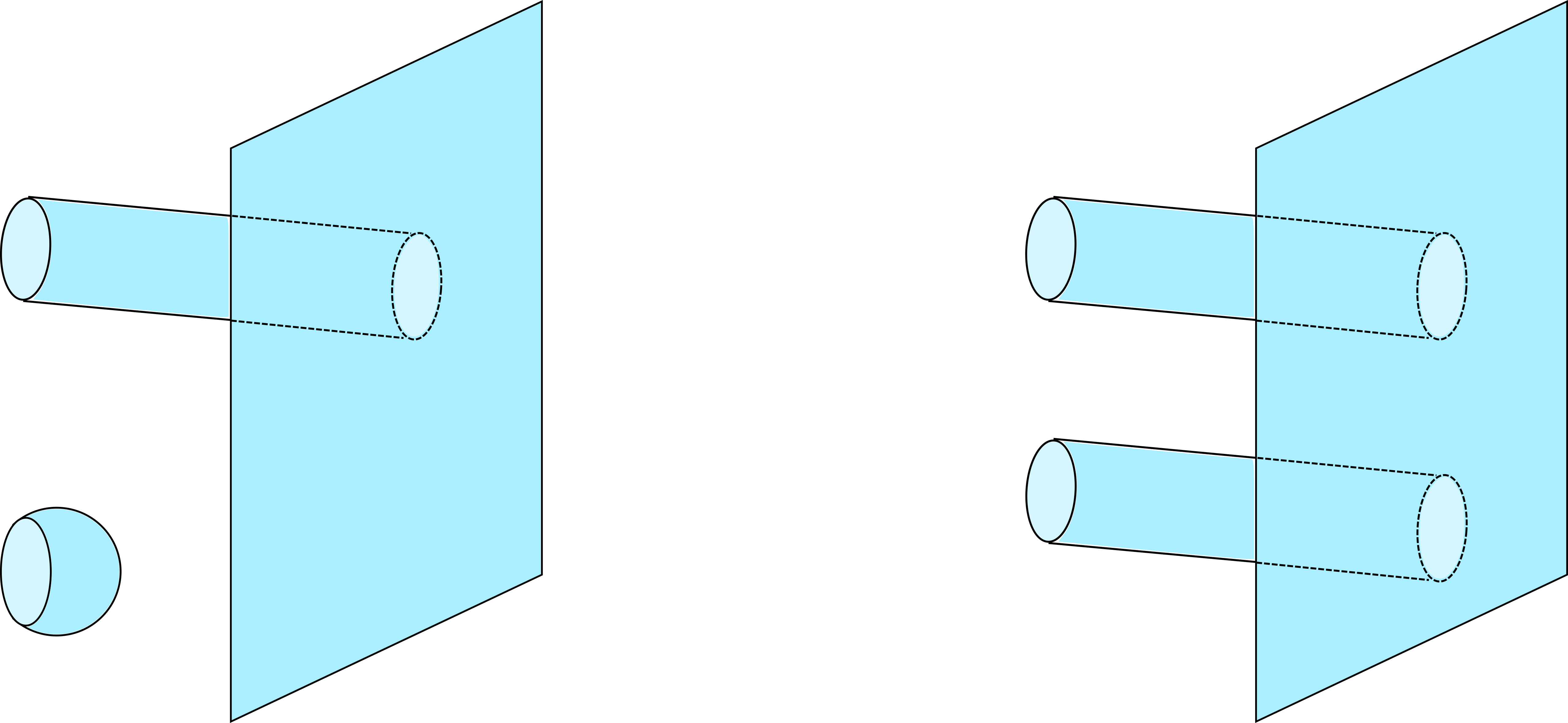
In the example (98), each term in $Y$ contains two $X_{i}$ legs, therefore we have

\displaystyle\frac{\left[Y(x)^{2}e^{\text{i}\sum_{i}k_{i}x_{i}}\right]}{\langle e^{\text{i}\sum_{i}k_{i}x_{i}}\rangle}=\frac{2\langle Y\rangle\langle Y(x)e^{\text{i}\sum_{i}k_{i}x_{i}}\rangle_{c}}{\langle e^{\text{i}\sum_{i}k_{i}x_{i}}\rangle}+\frac{\langle Y(x)e^{\text{i}\sum_{i}k_{i}x_{i}}\rangle_{c}^{2}}{\langle e^{\text{i}\sum_{i}k_{i}x_{i}}\rangle^{2}}+\frac{\langle Y(x)^{2}e^{\text{i}\sum_{i}k_{i}x_{i}}\rangle_{c}}{\langle e^{\text{i}\sum_{i}k_{i}x_{i}}\rangle}\,,

(146)

where the different terms correspond to one contraction to the brane, two separate contractions to the brane and a pair of connected contractions to the brane. The _c here means the contribution cannot be made disconnected if we only cut on the brane. Among these terms the last one is precisely the one missed in the previous proposal (63). A demonstration of these terms are shown in Figure 2. We notice that this approximation is closely related to the relation between $\hat{Z}$ and $\hat{W}$ discussed in Peng:2021vhs , see e.g. Figure. 9 there.

From this analysis, it is more obvious to understand why the Errors are all small when $\mu\neq 0$ in section 2.2.3. When disconnected contributions exist, the leading order contributions of the Error² always come from the disconnected component and hence the Error is guaranteed to be small. However, this is not very meaningful since as in most of the large- $N$ theories studied in the literature, we isolate away the disconnected contributions and always focus on the connected contributions.

2.3.2 Why the proposal works for the Pfaffian in the SYK model

From the above discussion, it seems that for a generic operators with complicated product structure, the original proposal (62) almost surely fails. However, we know from explicit computations in Saad:2021rcu ; Mukhametzhanov:2021nea that the approximation works well for the hyperpfaffian of the random couplings which is also related to the partition function of the SYK model.

We believe the reason for this is the large- $N$ factorizations properties due to large- $N$ constraints. By this we mean when the operators are defined to have extra structures, for example as a trace or a determinant over the $N$ flavors, such extra structure remains to affect the computation of the Error. When this is true, which indeed is our case, then the contractions between the two copies of Error are necessarily suppressed by the large- $N$ factors; either $1/N$ when the structure is trace as in (77) or higher powers of $1/N$ when the structure is a determinant. Therefore all contractions between the two copies of Errors are suppressed and at the leading order the result factorizes and hence the original proposal (62) works. ⁵⁵5A related fact is that when the approximation is no longer good the relation between the 4 ${}^{\text{th}}$ moment $\langle Y^{4}\rangle$ of the observable (98) and the second moment $\langle Y^{2}\rangle$ deviates significantly from the Gaussian distribution. In Gaussian distribution, this contribution is $3\langle Y^{2}\rangle\subset\langle Y^{4}\rangle$ , on the other hand, for the observable $Y$ in (98) we get $\displaystyle\langle Y^{4}\rangle$ $\displaystyle=$ $\displaystyle 8\sum_{i\neq j}\langle X_{i}^{4}X_{j}^{4}\rangle+60\sum_{i\neq j\neq p\neq q}\langle X_{i}^{2}X_{j}^{2}X_{p}^{2}X_{q}^{2}\rangle+48\sum_{i\neq j\neq p}\langle X_{i}^{4}X_{j}^{2}X_{p}^{2}\rangle$ (147) $\displaystyle\approx$ $\displaystyle 60N^{4}t^{8}\neq 3\langle Y^{2}\rangle^{2}-2\langle Y\rangle^{4}\approx 12N^{4}t^{8}\ .$ (148) But at the moment we have not succeeded in making a causal relation between this fact and the fact that the Error is small. The explanation in the main text does better in doing so.

A somewhat ad hoc reason for the need of traces or determinant in the definition of the operator to make the discussion about (half-)wormhole meaningful is the following. There is no “spacetime” in our statistical models, so we cannot use any locality property to identify a function of the random variables as a single operator; the most we can do is to use a trace or determinant structure to identify a group of random variables as an operator. If there is no such trace/determinant constraints, it is equally legitimate to regard the result as computing correlations of a large number of the fundamental random variables and the (half-)wormhole interpretation is not necessarily relevant.

A different interpretation of the importance of the existence of such trace or determinant structure could be considered as some emergent global symmetry among the random variables (probably when appropriately analytically continued). By this we simply mean if we treat the random variables $X_{i}$ as “fields”, then the action, ie the probability distribution, and the operators we considered in the computation all have $SO(N)$ symmetry among them. Then the invariant tensors of $SO(N)$ directly lead to the trace or determinant structures we just described. It is interesting to make this point more clear, and we plan to come back to this question somewhere else.

We did not find a general proof of the above assertion (145) or (146), but as a check we can, according to our assertion, modify the definition of the function $Y$ and put in by hand some constraints, mimicking a trace structure. Then we find with this constraints the approximation (62) is indeed valid. For instance we could introduce a restriction in the sum

\displaystyle Y=\sum_{i+j=M}X_{i}X_{j},\quad N<M<2N,\quad i\neq j\,,

(149)

where $N$ is the total number of $X$ ’s and $M$ is an integer. Without loss of generality we assume $M$ is even in the following, and the computation for odd $M$ is the same. Following the previous computations, we get

\displaystyle Y^{2}

\displaystyle=2\sum_{i+j=M}X_{i}^{2}X_{j}^{2}+\sum_{i\neq j\neq m\neq n}X_{i}X_{j}X_{m}X_{n}\,,

(150)

and

\displaystyle\langle Y\rangle=K\mu^{2},\quad\langle Y^{2}\rangle=2K(t^{2}+\mu^{2})^{2}+K(K-2)\mu^{4},\quad K=2N-M\ .

(151)

Taking $X_{i}$ from the same Gaussian distribution in the previous cases we get the expression for the error

\displaystyle\text{Error}=4t^{2}\sum_{i+j=M}X_{i}^{2}-4Kt^{4}-4Kt^{2}\mu^{2}.

(152)

It is straightforwardly to show that the expectation values

\displaystyle\langle\text{Error}\rangle=0\,,\qquad\langle(\text{Error}/4)^{2}\rangle=2Kt^{8}+4Kt^{6}\mu^{2}\ .

(153)

Clearly in this case $\langle(\text{Error}/4)^{2}\rangle$ is $1/N$ suppressed compared to $\langle Y^{2}\rangle^{2}$ independent on the value of $\mu$ . Hence the approximation (62) is always valid in the presence of this extra constraint. Similar restrictions could be imposed to models with general $q$ . It turns out that again the computation is quite similar and we expect the approximation to be valid in these cases too.

3 SYK at one time point: $\langle J_{a}\rangle=0$

In this section, we study the half-wormhole contributions in some 0d SYK model that can be considered as the usual 0+1d SYK model on a single instant of time. This section is largely a review of previous results in Saad:2021rcu ; Mukhametzhanov:2021nea ; Mukhametzhanov:2021hdi ; we provide more details of various saddle point results and carry out Lefschetz thimble analysis of some computations when needed.

3.1 SYK model with one time point

Let us first revisit the analysis of the 0-dimensional SYK model introduced in Saad:2021rcu . We are interested in the following Grassmann integral

\displaystyle z=\int d^{N}\psi\exp(\text{i}^{q/2}\sum J_{i_{1}\dots i_{q}}\psi_{i_{1}\dots i_{q}})\,,

(154)

where $\psi_{i_{1}\dots i_{q}}=\psi_{a_{1}}\psi_{a_{2}}\dots\psi_{a_{q}}$ and $\psi_{i}$ are Grassmann numbers. The number $z$ can be understood as the partition function of $0+0$ dimensional analogue of SYK model. The random couplings $J_{i_{1}\dots i_{q}}$ is drawn from a Gaussian distribution

\displaystyle\langle J_{i_{1}\dots i_{q}}\rangle=0,\quad\langle J_{i_{1}\dots i_{q}}J_{j_{1}\dots j_{q}}\rangle=t^{2}\delta_{i_{1}j_{1}}\dots\delta_{i_{q}j_{q}},\quad t^{2}=\frac{(q-1)!}{N^{q-1}}\ .

(155)

We sometimes use the collective indies $A,B$ to simplify the notation

\displaystyle A=\{a_{1}<\dots<a_{q}\}\,,\qquad J_{A}\psi_{A}\equiv J_{a_{1}\dots a_{q}}\psi_{a_{1}\dots a_{q}}\ .

(156)

Integrating out the Grassmann numbers directly gives (96)⁶⁶6Here we choose the measure of Grassmann integral to be $\int d^{N}\psi\psi_{1\dots N}=\text{i}^{-N/2}$ .:

\displaystyle z=\int d^{N}\psi\exp(\text{i}^{q/2}J_{A}\psi_{A})=\sum^{\prime}_{A_{1}<\dots<A_{p}}\text{sgn}(A)J_{A_{1}}\dots J_{A_{p}}\,,\quad p=N/q\,,

(157)

where the expression (157) is nothing but the hyperpfaffian $\text{Pf}(J)$ . Since $\langle z\rangle=0$ due to (155), we focus on $z^{2}$ and $\langle z^{2}\rangle$

	$\displaystyle z^{2}=z_{L}z_{R}=\int\text{d}^{N}\psi^{L}\text{d}^{N}\psi^{R}\exp\left\{\text{i}^{q/2}\sum_{A}J_{A}\left(\psi_{A}^{L}+\psi_{A}^{R}\right)\right\}\,,$		(158)
	$\displaystyle\langle z^{2}\rangle=\int\text{d}^{2N}\psi\exp\left\{\frac{N}{q}\left(\frac{1}{N}\sum_{i=1}^{N}\psi_{i}^{L}\psi_{i}^{R}\right)^{q}\right\}\,,$		(159)

where we have assumed that $q$ and $N$ are even. The exact values of (159) can be computed by introducing the standard $G,\Sigma$ variables

$\displaystyle\langle z^{2}\rangle$	$\displaystyle=$	$\displaystyle\int\text{d}^{2N}\psi\int_{\mathbb{R}}\text{d}G\delta\left(G-\frac{1}{N}\sum_{i=1}^{N}\psi_{i}^{L}\psi_{i}^{R}\right)\exp\left(\frac{N}{q}G^{q}\right)$	(160)
	$\displaystyle=$	$\displaystyle\int_{\mathbb{R}}\text{d}G\int_{\text{i}\mathbb{R}}\frac{\text{d}\Sigma}{2\pi\text{i}/N}\exp\left\{N\left(\log(\Sigma)-\Sigma G+\frac{1}{q}G^{q}\right)\right\}$	(161)
	$\displaystyle=$	$\displaystyle N^{-N}\int_{\mathbb{R}}\text{d}G\exp\left(\frac{N}{q}G^{q}\right)(-\partial_{G})^{N}\delta(G)$	(162)
	$\displaystyle=$	$\displaystyle\frac{N!(N/q)^{N/q}}{N^{N}(N/q)!}=e^{-(1-\frac{1}{q})N}\sqrt{q}\left(1+\frac{1-q}{12N}+\mathcal{O}(\frac{1}{N^{2}})\right)\,,$	(163)

where in the last step we expand around $N\to\infty$ to the next-to-leading order.

Next we consider the non-averaged quantity (158). Following Saad:2021rcu , we rewrite

\displaystyle z^{2}=\int_{R}\text{d}\sigma\Psi(\sigma)\Phi(\sigma)\,,\quad\Psi(\sigma)=\int\frac{dg}{2\pi/N}\exp[N(-\text{i}\sigma g-1/qg^{q})]\,,

(164)

where the coupling dependent piece $\Phi$ is

\displaystyle\Phi(\sigma)=\int\text{d}^{2N}\psi\exp\left\{\text{i}e^{-\frac{\text{i}\pi}{q}}\sigma\psi_{i}^{L}\psi_{i}^{R}+\text{i}^{q/2}J_{A}(\psi_{A}^{L}+\psi_{A}^{R})-\frac{N}{q}\left(\frac{1}{N}\psi_{i}^{L}\psi_{i}^{R}\right)^{q}\right\}\,.

(165)

Its averaged value is

\displaystyle\langle\Phi(\sigma)\rangle=(\text{i}e^{-\frac{\text{i}\pi}{q}}\sigma)^{N}\ .

(166)

As suggested in Saad:2021rcu , to understand the relation between each individual result and the averaged result, we could figure out in what region of the $\sigma$ -plane $\Phi$ is self-averaging. This is reflected in the quantity $\langle\left(\Phi(\sigma)-\langle\Phi(\sigma)\rangle\right)^{2}\rangle$ . Therefore we compare $\langle\Phi(\sigma)\rangle^{2}$ with $\langle\Phi(\sigma)^{2}\rangle$

\displaystyle\langle\Phi(\sigma)^{2}\rangle=\int_{R}\frac{\text{d}^{4}\sigma_{AB}\text{d}^{4}g_{AB}}{(2\pi/N)^{4}}e^{N\left[\log(-e^{-\frac{2\text{i}\pi}{q}}(\sigma^{2}+\sigma_{14}\sigma_{23}-\sigma_{13}\sigma_{24}))-\text{i}\sigma_{AB}g_{AB}-\frac{1}{q}g_{AB}^{q}\right]}\,,

(167)

where we relabel $L=1,L^{\prime}=3,R=2,R^{\prime}=4$ and $(AB)=(13),(14),(23),(24)$ . The integral can be done exactly Saad:2021rcu following a similar computation we used to get (163)

\displaystyle\langle\Phi(\sigma)^{2}\rangle=(-e^{-\frac{2\text{i}\pi}{q}})^{N}\sum_{n_{1}+n_{2}+n_{3}=\frac{N}{q},n_{i}\geq 0}\frac{N!}{N^{2q(n_{2}+n_{3})}}\left(\frac{N}{q}\right)^{2(n_{2}+n_{3})}\frac{\sigma^{2qn_{1}}(qn_{2})!(qn_{3})!}{(qn_{1})!(n_{2}!)^{2}(n_{3}!)^{2}}\,,

(168)

which can be organized into a polynomial in $\sigma$

	$\displaystyle\langle\Phi(\sigma)^{2}\rangle$	$\displaystyle=$	$\displaystyle(-e^{-\frac{2\text{i}\pi}{q}})^{N}\left(\sigma^{2N}+\frac{2N!q!}{(N-q)!q^{2}N^{2q-2}}\sigma^{2N-2q}+\dots+e^{2N\frac{1-q}{q}}2q\right)$		(169)
		$\displaystyle\sim$	$\displaystyle(-e^{-\frac{2\text{i}\pi}{q}})^{N}\left(\sigma^{2N}+\frac{2(q-1)!}{qN^{q-2}}\sigma^{2N-2q}+\dots+e^{2N\frac{1-q}{q}}2q\right)\,,$		(170)

where the phase factor is trivial whenever $q$ divides $N$ .

3.2 The saddle points analysis

The above results can be reproduced by saddle point approximation in large $N$ limit.

3.2.1 The averaged $\langle z^{2}\rangle$

To obtain the same result (163) from saddle point approximation, we first we rotate the contour

\displaystyle\Sigma=\text{i}e^{-\text{i}\frac{\pi}{q}}\sigma,\quad G=e^{\text{i}\frac{\pi}{q}}g\,,

(171)

to get

\displaystyle\langle z^{2}\rangle=\int_{R}\text{d}g\int_{R}\frac{\text{d}\sigma}{2\pi/N}\exp\left\{N\left(\log(\text{i}e^{-\frac{\text{i}\pi}{q}}\sigma)-\text{i}\sigma g-\frac{1}{q}g^{q}\right)\right\}\equiv\int_{R}\text{d}g\int_{R}\frac{\text{d}\sigma}{2\pi/N}e^{NS}\,,

(172)

so that the integral converges. The saddle point equations are

\displaystyle-\text{i}\sigma-g^{q-1}=0\,,\quad g^{q}=-1\,,\quad\rightarrow\quad g=e^{\frac{(2m+1)\text{i}\pi}{q}}\,,\quad m=0,\dots,q-1\ .

(173)

All of them give the same on-shell action

\displaystyle\langle z^{2}\rangle_{s}=\frac{N}{2\pi}e^{-(1-\frac{1}{q})N}\ .

(174)

To match with the exact result (163) we need to consider fluctuations around the saddle points. For simplicity let us take $q=4$ and focus on one of the saddle points

\displaystyle\sigma_{s}=g_{s}=-(-1)^{\frac{3}{4}},\quad\langle z^{2}\rangle_{s}=\frac{N}{2\pi}e^{-\frac{3}{4}N}.

(175)

Expanding the exponent around this saddle

\displaystyle\sigma=\sigma_{s}+x,\quad g=g_{s}+y

(176)

to the second order

\displaystyle S_{2}\sim-\frac{3}{4}+\frac{3\text{i}x^{2}}{2}-\text{i}xy-\frac{\text{i}y^{2}}{2}+[(-1)^{3/4}x^{3}+\frac{(-1)^{3/4}}{3}y^{3}]+\frac{y^{4}-x^{4}}{4}\,,

(177)

and evaluating the integral directly gives the fluctuation that combines with the saddle contribution to

\displaystyle\langle z^{2}\rangle_{\text{saddle}+\text{loop}}=e^{-\frac{3}{4}N}\frac{1}{2}\left(1-\frac{1}{4N}\right)\ .

(178)

Adding contributions from all 4 saddles we arrive at

\displaystyle\langle z^{2}\rangle_{\text{saddle}+\text{loop}}=2e^{-\frac{3}{4}N}\left(1-\frac{1}{4N}\right)\,,

(179)

that agrees with (163) at the two-loop order.

3.2.2 The unaveraged $z^{2}$ : the wormhole saddle

The result (170) can be reproduced from a saddle point analysis in the large- $N$ limit. The saddle point equations are

\displaystyle g_{AB}^{q-1}=-\text{i}\sigma_{AB}\,,\quad-\text{i}g_{13}=\frac{\sigma_{24}}{f},\quad\text{i}g_{14}=\frac{\sigma_{23}}{f},\quad\text{i}g_{23}=\frac{\sigma_{14}}{f},\quad-\text{i}g_{24}=\frac{\sigma_{13}}{f}\,,

(180)

where $f\equiv\sigma_{14}\sigma_{23}-\sigma_{13}\sigma_{24}+\sigma^{2}$ . The trivial solution $\sigma_{AB}=g_{AB}=0$ leads to

\displaystyle\langle\Phi(\sigma)^{2}\rangle_{\text{trivial}+1\text{loop}}=\langle\Phi(\sigma)\rangle^{2}\,,

(181)

which says the trivial saddle always agrees with the first term in (170).

Next let us consider non-trivial solutions with $\sigma_{AB}\neq 0$ . From the equations of motion we obtain

	$\displaystyle x^{q-2}=y^{q-2},\quad(x^{q-1}-y^{q-1}+\sigma^{2})^{2}=x^{q-2}=y^{q-2}\,,$		(182)
	$\displaystyle g_{13}^{q}=g_{24}^{q},\quad g_{23}^{q}=g_{14}^{q}$		(183)

where

\displaystyle x=g_{13}g_{24},\quad y=g_{14}g_{23}\ .

(184)

It is easy to check that solutions of the above equation satisfies $x=ye^{\frac{2m\pi\text{i}}{q-2}}$ , and for each choice of $m$ there are $2q^{2}$ solutions of $g_{ab}$ . For simplicity let us again focus on the $q=4$ case such that there are only two classes $x=\pm y$ .

$\bullet$ When $x=y$ we find another 32 non-trivial saddles. The on-shell action of all of them are the same

\displaystyle\langle\Phi(\sigma)^{2}\rangle_{\text{non-trivial}}^{+}=N^{4}\langle\Phi(\sigma)\rangle^{2}=\langle\Phi(\sigma)^{2}\rangle_{\text{trivial}}\,,

(185)

where the factor $N^{4}$ comes from the measure of (167). However the 1-loop fluctuations around them are different

\displaystyle\text{trivial saddle}:\frac{1}{N^{4}}\,,\quad\text{non-trivial saddles}:\frac{1}{8N^{4}}\ .

(186)

We notice that including the 1-loop effect, the trivial saddle is larger and it reproduces the large $N$ behavior of the exact result. On the other hand, the non-trivial saddle contributions are also comparable; so it is possible that we should also take into account of their contributions as well. However, if we add all the trivial and non-trivial saddle-point values, the result will obviously exceed the exact value (170). In fact, by a simple Lefschetz-thimble analysis, see e.g. Witten:2010cx , which is reviewed In Appendix E, we conclude that these non-trivial saddles should not be included.

In particular, we choose a Morse function to be the real part of the action (167)

$\displaystyle h\equiv\Re(S)=$	$\displaystyle\sum_{abj}\left(-\frac{g_{abj}^{4}}{4}+\frac{3g_{ab1}^{2}g_{ab2}^{2}}{2}+g_{ab1}\sigma_{ab2}+g_{ab2}\sigma_{ab1}\right)$
	$\displaystyle\quad+\frac{1}{2}\log\left((\sigma_{142}\sigma_{231}+\sigma_{141}\sigma_{232}-\sigma_{132}\sigma_{241}-\sigma_{131}\sigma_{242})^{2}\right.$
	$\displaystyle\left.\quad+(1+\sigma_{141}\sigma_{231}-\sigma_{142}\sigma_{232}-\sigma_{131}\sigma_{241}+\sigma_{132}\sigma_{242})^{2}\right)\,,$	(187)

where we have chosen $q=4$ for simplicity and $\sigma=1$ since we are interested in the case $\sigma\neq 0$ ⁷⁷7The $\sigma=0$ case is analyzed in Saad:2021rcu . The $g_{abi}$ and $\sigma_{abj}$ are the real and imaginary parts of the field $g_{ab}$ and $\sigma_{ab}$

\displaystyle g_{ab}=g_{ab1}+\text{i}g_{ab2},\quad\sigma_{ab}=\sigma_{ab1}+\text{i}\sigma_{ab2}\ .

(188)

The downward flow equations of the Morse function are

\displaystyle\frac{dg_{abj}}{dt}=-\frac{\partial h}{\partial g_{abj}},\quad\frac{d\sigma_{abj}}{dt}=-\frac{\partial h}{\partial\sigma_{abj}}\ .

(189)

The end point of each anti-thimble is one of the saddles at $g_{abj}^{c}$ and $g_{abj}^{c}$ , which leads to the following boundary conditions of the flow equation

\displaystyle\lim_{t\to+\infty}g_{abj}=g_{abj}^{c},\quad\lim_{t\to+\infty}\sigma_{abj}=\sigma_{abj}^{c}\ .

(190)

We can then solve the flow equation and obtain the Lefschetz anti-thimbles going through each saddle point and if they intersect with the original integration contour the saddle point contributes to the integral.

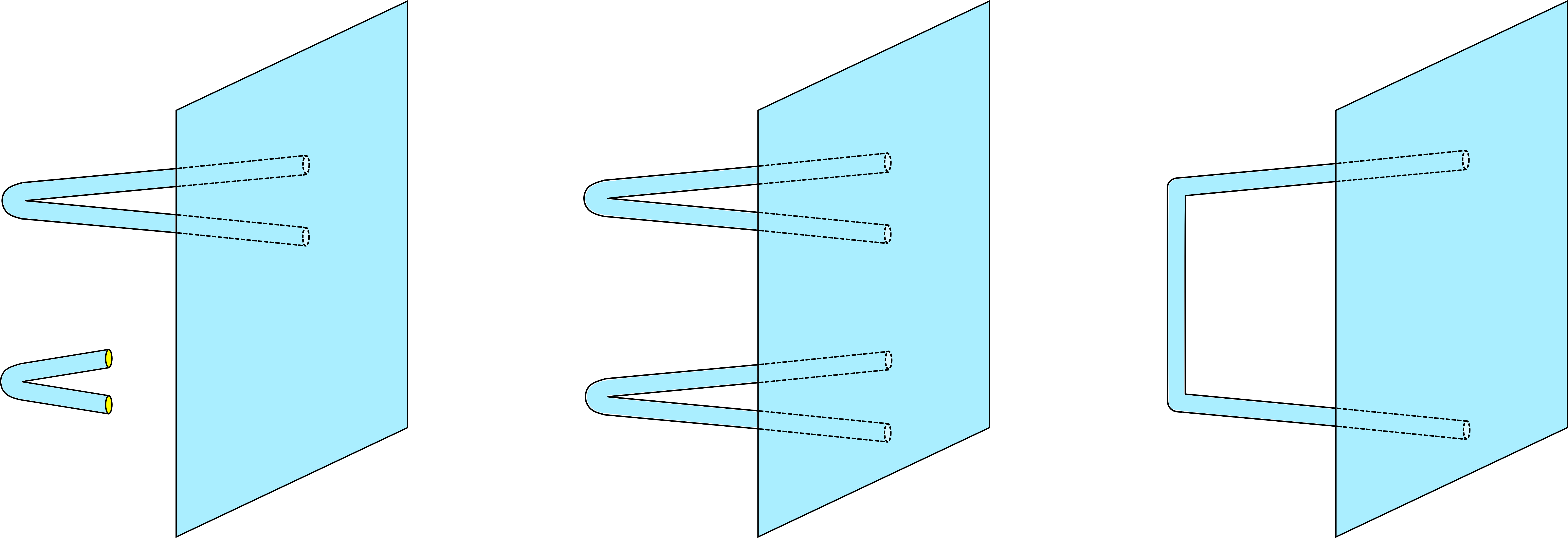
For example in Figure 3 we illustrate examples of the anti-thimbles of the saddle point

	$\displaystyle g_{13}=1,\quad g_{24}=-1,\quad g_{14}=(-1)^{3/4},\quad g_{23}=(-1)^{1/4},$		(191)
	$\displaystyle\sigma_{13}=\text{i},\quad\sigma_{24}=-\text{i},\quad\sigma_{14}=(-1)^{3/4},\quad\sigma_{23}=-(-1)^{1/4}\,,$		(192)

that do not intersect with the original integration contour, namely the real axis. This means the contribution of this saddle should not be included to the integral.

Examples of anti-thimbles of another saddle point

	$\displaystyle g_{13}=-(-1)^{1/4},\quad g_{24}=(-1)^{3/4},\quad g_{14}=-1,\quad g_{23}=-1,$		(193)
	$\displaystyle\sigma_{13}=(-1)^{1/4},\quad\sigma_{23}=(-1)^{3/4},\quad\sigma_{14}=-\text{i},\quad\sigma_{23}=-\text{i}\,,$		(194)

is shown in Figure 4. Again they do not intersect with the real axis so the contribution from this saddle should not be included either.

We can run this analysis over all the nontrivial saddles and find none of them contribute to the integral. As a result, the path integral can be approximated entirely by the trivial saddle.

$\bullet$ When $x=-y$ , there are also nontrivial saddle points and a similar analysis of Lefschetz thimbles demonstrate that they do not contribute to the integral.

Actually, there is a quicker way to arrive at the same conclusion. We find that the on-shell actions corresponding to these saddle points are

\displaystyle\left(\frac{\sigma^{2}}{2}\right)^{\frac{N}{3}}e^{-N\pm\frac{3}{2}2^{\frac{1}{3}}Ne^{\frac{2\text{i}m\pi}{3}}\sigma^{\frac{4}{3}}},\quad m=0,\pm 1,\quad\sigma\rightarrow\infty\ .

(195)

However these saddle points should be saddle points of the entire multi-dimensional integral including the integral over $\sigma$ . As a result this saddle should also satisfy the fall-off condition of the $\sigma$ integral, otherwise they will not contribute to the $\sigma$ integral. Therefore we should only consider the decaying saddle points namely

\displaystyle\left(\frac{\sigma^{2}}{2}\right)^{\frac{N}{3}}e^{-N+\frac{3}{2}2^{\frac{1}{3}}Ne^{\pm\frac{2\text{i}\pi}{3}}\sigma^{\frac{4}{3}}},\quad\left(\frac{\sigma^{2}}{2}\right)^{\frac{N}{3}}e^{-N-\frac{3}{2}2^{\frac{1}{3}}N\sigma^{\frac{4}{3}}}\ .

(196)

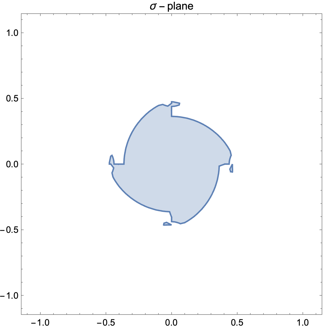
We plot the region where these non-trivial saddle dominates over the trivial saddle in Figure 5, and it is easy to observe from the figure that the wormhole saddle (317) of $\langle z^{2}\rangle$ , located at $|\sigma|=1$ , is in the region where the trivial saddle dominates.

Another family of solutions to the equation of motion (180) has $x=0$ or $y=0$ . On shell actions on these saddles behave as

\displaystyle\sigma^{\frac{2N}{3}}e^{-N+\frac{3}{2}Ne^{\pm\frac{2\text{i}\pi}{3}}\sigma^{\frac{4}{3}}},\quad\sigma^{\frac{2N}{3}}e^{-N-\frac{3}{2}N\sigma^{\frac{4}{3}}}\,,

(197)

whose dominant regions are similar to Figure 5 and they are sub-leading comparing with the trivial saddle.

Putting all the result together we confirm that the trivial saddle point dominate in the $g_{ab}$ and $\sigma_{ab}$ integral and the wormhole saddle (317) is self-averaging.

3.2.3 The unaveraged $z^{2}$ : the linked half-wormhole saddles

The trivial saddle point discussed in the previous section gives vanishing contribution at $\sigma\sim 0$ , so we expect other saddle points dominate the path integral here. In Saad:2021rcu they are referred to as the (linked) half-wormhole saddles. Here we provide some further details of the saddle contribute at $\sigma\sim 0$ and show that it agrees with the exact result in (170), ie

\displaystyle\langle\Phi(0)^{2}\rangle_{\text{ext}}\sim 2qe^{-\frac{3}{2}N}\ .

(198)

We can apply the same analysis, except that now we evaluate at $\sigma\sim 0$ , as in the previous section. As expected, the trivial saddle gives

\displaystyle e^{N\log(\sigma)}\sim 0\ .

(199)

The subleading non-trivial saddles (196) and (197) discussed in the previous section has on-shell values

\displaystyle\frac{e^{-\frac{3}{2}N}}{2^{N/2}},\quad e^{-\frac{3}{2}N}\ ,

(200)

respectively when $\sigma=0$ . So (197) dominates. Adding them up precisely gives the exact solution (198)

\displaystyle 2qe^{-\frac{3}{2}N}\,,

(201)

The general lesson is that the linked half wormhole saddle points are always in the integral, and furthermore they are also always saddles. It’s only that they are, for most of the time, hidden behind the leading saddles. They can only be exposed in regions where the leading saddle decreases faster, namely the $\sigma\sim 0$ region in this case.

4 SYK at one time point: $\langle J_{a}\rangle\neq 0$

In the following, we will generalize the study of half-wormhole along several directions. The main question we want to address is how the distribution of the random coupling affects the wormhole and half-wormhole saddles.

First let us consider the case where the random coupling is drawn from a general Gaussian distribution ${\cal N}(u,t^{2})$ ⁸⁸8When we write $J_{A}$ , we have in mind that the index set $A$ is automatically sorted, and all $J$ ’s with other permutations of $A$ picks up signs accordingly.

\displaystyle\langle J_{A}\rangle=J_{A}^{0}=u,\quad\langle J_{A}^{2}\rangle-\langle J_{A}\rangle^{2}=\tau^{2}\frac{(q-1)!}{N^{q-1}}\equiv t^{2}\,,

(202)

in particular, the mean value of the random coupling could be non-vanishing.

The ensemble averaged quantities can be computed directly by first averaging over the couplings and then integrating out the fermions

$\displaystyle\langle z\rangle$	$\displaystyle=$	$\displaystyle\text{PF}(J^{0})\,,$	(203)
$\displaystyle\langle z^{2}\rangle$	$\displaystyle=$	$\displaystyle\int d^{2N}\psi\exp\left(\text{i}^{q}t^{2}\sum_{A}\psi_{A}^{L}\psi_{A}^{R}+\text{i}^{q/2}J_{A}^{0}(\psi_{A}^{L}+\psi_{A}^{R})\right)$	(204)
	$\displaystyle=$	$\displaystyle\sum^{\prime}_{A,B}\text{sgn}(A)\text{sgn}(B)\left(J_{A_{1}}^{0}J_{B_{1}}^{0}+\delta_{A_{1}B_{1}}t^{2})\right)\dots\left(J_{A_{p}}^{0}J_{B_{p}}^{0}+\delta_{A_{p}B_{p}}t^{2})\right)\ .$	(205)

4.1 Half-wormhole saddle in $z$

Since $\langle z\rangle\neq 0$ , we expect a disk saddle point in the path integral presentation of $z$ that gives the contribution of $\langle z\rangle$ . Moreover, like linked half-wormhole contribution to $z^{2}$ in the model with $u=0$ , it is possible that there are also single half-wormhole saddles contributing to $z$ , ⁹⁹9This single half-wormhole saddle is related to the half-wormhole saddle of JT gravity introduced in Blommaert:2021fob . as shown in Figure. 6. We will show in the following that such saddles indeed exist and together with their contribute $\Theta_{1}$ the following approximation is good

\displaystyle z\approx\langle z\rangle+\Theta_{1}\ .

(206)

Let us clarify the notation we use in this paper, we call the non-self-averaged component in $z$ as “single half-wormhole” or simply “half-wormhole”, and we refer to the non-self-averaged saddle in $z^{2}$ as “linked half-wormhole”.

To demonstrate (206) explicitly, recall that the partition function is given by

\displaystyle z=\int\text{d}^{N}\psi\exp\left(\text{i}^{q/2}\sum J_{i_{1}\dots i_{q}}\psi_{i_{1}\dots i_{q}}\right)\ .

(207)

The ensemble averaged quantity $\langle z\rangle$ does not vanish

\displaystyle\langle z\rangle=\int\text{d}^{N}\psi\exp(\text{i}^{q/2}\sum J^{(0)}_{i_{1}\dots i_{q}}\psi_{i_{1}\dots i_{q}})=u^{p}\frac{(pq/2)!}{p!((q/2)!)^{p}}\equiv m_{p}u^{p}\,,\quad pq=N\ .

(208)

In the following we present a heuristic but simple proof of this result. A more rigorous but technical proof is presented in Appendix G. For simplicity let us first consider the $q=4$ case

\displaystyle\langle z\rangle=\int d^{N}\psi\,e^{-u\sum_{A}\psi_{A}},\quad A=\{a_{1}<\dots<a_{4}\}\ .

(209)

We introduce the collective variable $G$

\displaystyle G=\frac{1}{N}\sum_{1\leq i<j\leq N}\psi_{i}\psi_{j},\quad G^{2}=\frac{2!}{N^{2}}\sum_{A}\psi_{A}\,,

(210)

then $\langle z\rangle$ can be rewritten as

\displaystyle\langle z\rangle=\int_{\mathbb{R}}\text{d}G\int_{\text{i}\mathbb{R}}\frac{d\Sigma}{2\pi\text{i}/N}\text{d}^{N}\psi\,e^{-\frac{u}{2}N^{2}G^{2}}e^{-\Sigma(NG-\sum_{i<j}\psi_{i}\psi_{j})}\ .

(211)

Now we can integrate the out the fermions to get

\displaystyle\int d^{N}\psi\,e^{\Sigma\sum_{i<j}\psi_{i}\psi_{j}}=(\Sigma)^{N/2}m_{p}\,|_{(q=2)}=\Sigma^{N/2}\ .

(212)

Then (211) becomes

	$\displaystyle\langle z\rangle_{q=4}$	$\displaystyle=$	$\displaystyle\int_{\mathbb{R}}\text{d}G\int_{\text{i}\mathbb{R}}\frac{d\Sigma}{2\pi\text{i}/N}\Sigma^{N/2}e^{-\frac{uN^{2}G^{2}}{2}}e^{-N\Sigma G}\,$		(213)
		$\displaystyle=$	$\displaystyle N^{-N/2}(\partial_{G})^{N/2}e^{-\frac{uN^{2}G^{2}}{2}}\,\|_{G=0}\,=\left(\frac{u}{2}\right)^{N/4}\frac{(N/2)!}{(N/4)!}=m_{p}u^{p}\|_{q=4}\,.$		(213)

For general $q$ , the proof is similar with the modification

\displaystyle\sum_{A}\psi_{A}=\frac{N^{q/2}}{(q/2)!}G^{q/2}\,.

(214)

In summary, we have generalized the $G,\Sigma$ trick and derived an effective action to compute $\langle z\rangle$ :

\displaystyle\langle z\rangle=\int_{\mathbb{R}}\text{d}G\int_{\text{i}\mathbb{R}}\frac{d\Sigma}{2\pi\text{i}/N}\Sigma^{N/2}e^{u\text{i}^{q/2}\frac{N^{q/2}}{(q/2)!}G^{q/2}}e^{-N\Sigma G}\,.

(215)

It would be convenient to rotate the integral contour as

\displaystyle\Sigma\rightarrow\text{i}e^{-\text{i}\frac{2\pi}{q}}\sigma,\quad G\rightarrow e^{\text{i}\frac{2\pi}{q}}g

(216)

such that we obtain a “standard” action:

\displaystyle\langle z\rangle=\int_{\mathbb{R}}\frac{dgd\sigma}{2\pi/N}\exp\left\{\frac{N}{2}\left(\log(\text{i}e^{-\frac{2\pi\text{i}}{q}}\sigma)-2\text{i}\sigma g-\frac{2\mu}{q}g^{q/2}\right)\right\},

(217)

where we define

\displaystyle\mu\equiv\text{i}^{q/2}u\frac{2{N}^{q/2-1}}{(q/2-1)!},\quad\leftrightarrow\quad u=(-\text{i})^{q/2}\mu\frac{(q/2-1)!}{2N^{q/2-1}}.

(218)

Rescaling $\mu$ to 1, the saddle point equations are then

\displaystyle\frac{1}{\sigma}-2\text{i}g=0,\quad-2\text{i}\sigma-\mu g^{q/2-1}=0,\quad\rightarrow\quad\mu g^{q/2}=-1\ .

(219)

Comparing (217) with (172) it is easy to find that to reproduce the exact result (208) we have to added the contributions from all the $q/2$ saddles.

Having found the suitable saddle contributions to the averaged partition function $\langle z\rangle$ , we proceed to analyze the difference between the non-averaged quantity and the mean value $z-\langle z\rangle$ . We start with inserting the identity

\displaystyle 1=\int_{-\infty}^{\infty}dG_{h}\int_{-\text{i}\infty}^{\text{i}\infty}\frac{Nd\Sigma_{h}}{2\pi\text{i}}e^{-\Sigma_{h}(NG_{h}-\sum_{i<j}\psi_{i}\psi_{j})+\frac{N\mu}{q}\left(G_{h}^{q/2}-\left(\frac{1}{N}\sum_{i<j}\psi_{i}\psi_{j}\right)^{q/2}\right)}\,,

into the non-averaged partition function $z$ . To make the integral well defined, we again rotate the contour by $\Sigma_{h}=\text{i}e^{-2\text{i}\pi/q}\sigma_{h},G_{h}=e^{2\text{i}\pi/q}g_{h}$ , then $z$ can be cast into the form

\displaystyle z=\int_{-\infty}^{\infty}\frac{N\text{d}\sigma_{h}}{2\pi}\Psi(\sigma_{h})\hat{\Theta}(\sigma_{h})\,,

(221)

where the first factor is similar to (164)

\displaystyle\Psi(\sigma_{h})=\int_{\mathbb{R}}\frac{\text{d}g_{h}}{2\pi/N}\exp[N(-\text{i}\sigma_{h}g_{h}-\frac{\mu}{q}g_{h}^{q/2})]\,,

(222)

and the second factor is

\displaystyle\hat{\Theta}(\sigma_{h})=\int\text{d}^{N}\psi\exp[\text{i}e^{-\frac{2\text{i}\pi}{q}}\sigma_{h}\sum_{i<j}\psi_{i}\psi_{j}+\text{i}^{q/2}J_{A}\psi_{A}-\text{i}^{q/2}u\sum_{A}\psi_{A}]\ .

(223)

Averaging over the coupling, we get back to the computation in (217) where $\sigma_{h}=\frac{1}{2i}\left(\mu^{-2/q}e^{4\pi i(n+\frac{1}{2})/q}\right)$ . We expect a separate saddle point to appear in this integral which leads to the difference $z-\langle z\rangle$ . The $\Psi(\sigma_{h})$ is peaked at $\sigma_{h}=0$ , so we look for dominant contributions around $\sigma_{h}\approx 0$ , which is

\displaystyle\Theta_{1}=\hat{\Theta}(0)=\text{Pf}(J-J^{0})=\sum^{\prime}_{A}\text{sgn}(A)(J_{A_{1}}-J_{A_{1}}^{0})\dots(J_{A_{p}}-J_{A_{p}}^{0})\ .

(224)

It is clear that its average vanishes $\langle\Theta_{1}\rangle=0$ . Then we propose the approximation

\displaystyle z\approx\langle z\rangle+\Theta_{1}\ .

(225)

which is (206). According to the power of $J^{0}_{A}=u$ , we can further expand

\displaystyle\Theta_{1}

\displaystyle=\sum_{k=0}^{p}\Theta_{1}^{(k)}u^{k}\ .

(226)

To verify this approximation, we define the error function

\displaystyle\text{Error}=z-\langle z\rangle-\Theta_{1}\ .

(227)

A direct calculation gives

\displaystyle\langle\text{Error}^{2}\rangle=\langle z^{2}\rangle-\langle z\rangle^{2}+\langle\Theta^{2}\rangle-2\langle z\Theta\rangle

(228)

The quantities $\langle z^{2}\rangle,\langle\Theta^{2}\rangle,\langle z\Theta\rangle$ can be computed with the Feynman diagrams as shown in Fig. 7.

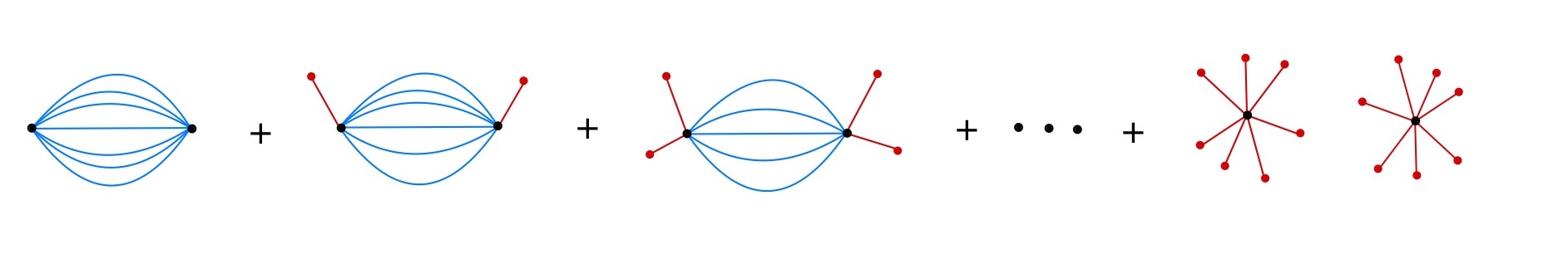
Recall that value of $\langle z\rangle$ is given by the star diagram that is one connected component of the last term in Fig. 7

\displaystyle\langle z\rangle=\frac{(pq/2)!}{p!((q/2)!)^{p}}\mu^{p}\equiv m_{p}\mu^{p}\,,

(229)

The value of $\langle z^{2}\rangle$ can be computed either from summing over the diagrams,

\displaystyle\langle z^{2}\rangle=\sum_{k=0}^{p}c_{k}m_{p-k}^{2}t^{2k}u^{2p-2k}\equiv\sum_{k}z_{2}^{(k)}\,,

(230)

where

\displaystyle c_{k}=\frac{1}{k!}{N\choose q}{N-q\choose q}\dots N-(k-1)q\choose q=\frac{N!}{k!(q!)^{k}(N-kq)!}\,,

(231)

or by introducing the collective variables

\displaystyle G_{LR}=\frac{1}{N}\sum_{i}\psi_{i}^{L}\psi_{i}^{R},\quad G_{L}=\frac{1}{N}\sum_{i<j}\psi_{i}^{L}\psi_{j}^{L},\quad G_{R}=\frac{1}{N}\sum_{i<j}\psi_{i}^{R}\psi_{j}^{R}\,,

(232)

and doing the path integral

$\displaystyle\langle z^{2}\rangle$	$\displaystyle=$	$\displaystyle\int_{R}\text{d}^{3}G_{i}\int_{\text{i}\mathbb{R}}d^{3}\Sigma_{i}\,e^{\frac{N}{q}(\tau^{2}G_{LR}^{q}+\mu G_{L}^{q/2}+\mu G_{R}^{q/2})-N(\Sigma_{i}G_{i})}\int\text{d}^{2N}\psi e^{\frac{1}{2}{\Psi}M{\Psi}},$
	$\displaystyle=$	$\displaystyle\int_{R}\text{d}^{3}G_{i}\int_{\text{i}\mathbb{R}}d^{3}\Sigma_{i}\,e^{\frac{N}{q}(\tau^{2}G_{LR}^{q}+\mu G_{L}^{q/2}+\mu G_{R}^{q/2})-N(\Sigma_{i}G_{i})}\sqrt{\text{det}[\Sigma_{L}\Sigma_{R}A^{2}+\Sigma_{LR}^{2}]}$
	$\displaystyle=$	$\displaystyle\int_{R}\text{d}^{3}G_{i}\int_{\text{i}\mathbb{R}}d^{3}\Sigma_{i}\,e^{\frac{N}{q}(\tau^{2}G_{LR}^{q}+\mu G_{L}^{q/2}+\mu G_{R}^{q/2})-N(\Sigma_{i}G_{i})}\text{det}[\text{i}\sqrt{\Sigma_{L}\Sigma_{R}}A+\Sigma_{LR}]$
	$\displaystyle=$	$\displaystyle\int_{R}\text{d}^{3}G_{i}\int_{\text{i}\mathbb{R}}d^{3}\Sigma_{i}\,e^{\frac{N}{q}(\tau^{2}G_{LR}^{q}+\mu G_{L}^{q/2}+\mu G_{R}^{q/2})-N(\Sigma_{i}G_{i})}\frac{1}{2}\left((\Sigma_{LR}+\text{i}\sqrt{\Sigma_{L}\Sigma_{R}})^{N}+(\Sigma_{LR}-\text{i}\sqrt{\Sigma_{L}\Sigma_{R}})^{N}\right)$
	$\displaystyle=$	$\displaystyle\int_{R}\text{d}^{3}G_{i}\int_{\text{i}\mathbb{R}}d^{3}\Sigma_{i}\,\sum_{m=0}^{N/2}{N\choose 2m}(\Sigma_{LR})^{2m}(\text{i}^{2}\Sigma_{L}\Sigma_{R})^{\frac{N}{2}-m}e^{\frac{N}{q}(\tau^{2}G_{LR}^{q}+\mu G_{L}^{q/2}+\mu G_{R}^{q/2})}e^{-N(\Sigma_{i}G_{i})}\,,$

where we have defined

	$\displaystyle\Psi=\left(\psi_{1}^{L},\dots,\psi_{N}^{L},\psi_{1}^{R},\dots,\psi_{N}^{R}\right),\quad M=\begin{pmatrix}\Sigma_{L}A&\Sigma_{LR}I_{N}\\ -\Sigma_{LR}I_{N}&\Sigma_{R}A\\ \end{pmatrix},$		(234)
	$\displaystyle A=-A^{T},\quad A_{ij}=1,\quad\forall i<j.$		(235)

Using the same tricks as (213), (4.1) can be evaluated exactly as

$\displaystyle\langle z^{2}\rangle$	$\displaystyle=$	$\displaystyle N^{-N}\sum_{k=0}^{p}{N\choose kq}(\partial_{G_{LR}})^{kq}(\text{i}^{2}\partial_{G_{L}}\partial_{G_{R}})^{\frac{N-kq}{2}}e^{\frac{N}{q}(\tau^{2}G_{LR}^{q}+\mu G_{L}^{q/2}+\mu G_{R}^{q/2})}\|_{G_{i}=0}$	(236)
	$\displaystyle=$	$\displaystyle N^{-N}\sum_{k=0}^{p}\text{i}^{N-kq}{N\choose kq}\frac{(kq)!}{k!}\left(\frac{N\tau^{2}}{q}\right)^{k}\left[\frac{(\frac{q(p-k)}{2})!}{(p-k)!}\right]^{2}\left(\frac{N\mu}{q}\right)^{2p-2k}$	(237)
	$\displaystyle=$	$\displaystyle\sum_{k=0}^{p}c_{k}m_{p-k}^{2}t^{2k}u^{2p-2k},$	(238)

which agrees with (230) as it should be.

Furthermore, from this result we find $z_{2}^{(0)}=\langle z\rangle^{2}$ which is given by the last diagram in Fig. 7 and $z_{2}^{(p)}=\langle z^{2}\rangle_{\mu=0}$ which is given by the first diagram in Fig. 7. The expression of $\Theta_{1}$ (224) implies that $\langle\Theta_{1}^{2}\rangle=\langle\Theta_{1}z\rangle=z_{2}^{(p)}$ , therefore we find

\displaystyle\langle\text{Error}^{2}\rangle=\sum_{k=1}^{p-1}c_{k}m_{p-k}^{2}t^{2k}u^{2p-2k}\equiv\sum_{k=1}^{p-1}z_{2}^{(k)}\,,

(239)

where $m_{p}$ is defined in (208). In the large- $N$ limit, some of the terms in the summation (230) dominate. If $z_{2}^{(p)}$ or $z_{2}^{(0)}$ dominates then the error is small.

However the dominant term is not always given by a fixed $z_{2}^{(k)}$ . A simple argument is the following. To find the dominant term we can compute the ratio¹⁰¹⁰10Recall that $p=N/q$ .

	$\displaystyle r_{k}=\frac{z_{2}^{(k)}}{z_{2}^{(k-1)}}=\frac{t^{2}(-k+p+1)(-4k+4p+1)(-4k+4p+3)}{3u^{2}(2k(p-k)+k)}\,,$		(240)
	$\displaystyle r_{p}=\frac{t^{2}}{pu^{2}},\quad r_{1}\sim\frac{p^{2}t^{2}}{u^{2}}\,,$		(241)

here for simplicity we have chosen $q=4$ . First we notice that $r_{k}$ decreases with respect to $k$ . Therefore if $r_{1}\leq 1$ i.e.

\displaystyle\frac{u}{t}\geq{p}\,,

(242)

then the dominant term will be $z_{2}^{(0)}$ . It means that all the wormhole saddles are suppressed. However if $r_{p}\geq 1$ i.e.

\displaystyle\frac{u}{t}\leq\frac{1}{\sqrt{p}}

(243)

then the dominant term will be $z_{2}^{(p)}$ , in other words the effect of $\mu$ can be neglected. For other cases with

\displaystyle\frac{1}{\sqrt{p}}<\frac{u}{t}<p,

(244)

by fine tuning the value of $u/t$ , every diagram in Fig. (7) is possible to be dominant. For the choices (202) and (218) which lead to reasonable large $N$ behavior we have

\displaystyle\frac{u}{t}\sim\frac{\mu}{\tau}\frac{(q/2-1)!}{\sqrt{(q-1)!}}N^{\frac{1}{2}}\sim\sqrt{p},

(245)

which exactly lies in the (244). It also implies there should be other saddles contributing to (223).

On the other hand, the can derive the saddle point equations

	$\displaystyle G_{L(R)}^{-1+\frac{q}{2}}=\frac{2}{\mu}\Sigma_{L(R)},\quad G_{LR}^{-1+q}=\frac{1}{\tau^{2}}\Sigma_{LR},$		(246)
	$\displaystyle G_{L(R)}=\frac{\text{i}\Sigma_{R(L)}}{2\sqrt{\Sigma_{L}\Sigma_{R}}}\frac{f_{+}^{n-1}-f_{-}^{n-1}}{f_{+}^{n}+f_{-}^{n}},\quad G_{LR}=\frac{f_{+}^{n-1}+f_{-}^{n-1}}{f_{+}^{n}+f_{-}^{n}}\,,$		(247)

where $f_{\pm}=\Sigma_{LR}\pm\text{i}\sqrt{\Sigma_{L}\Sigma_{R}}$ . Again for simplicity we will choose $\tau^{2}=\mu=1$ . There are always two types of trivial solutions

	$\displaystyle\text{wormhole solution}:\quad G_{L}=G_{R}=0,\quad G_{LR}=e^{\frac{2\text{i}m\pi}{q}},$		(248)
	$\displaystyle\text{disconnect solution}:\quad G_{LR}=0,\quad G_{L}=e^{\frac{4\text{i}m_{L}\pi}{q}},\quad G_{R}=e^{\frac{4\text{i}m_{R}\pi}{q}}$		(249)

with on-shell action

	$\displaystyle\text{wormhole solution}:\quad\langle z^{2}\rangle_{\text{wh}}=e^{-N(1-\frac{1}{q})}e^{\frac{2\text{i}m\pi N}{q}}$		(250)
	$\displaystyle\text{disconnect solution}:\quad\langle z^{2}\rangle_{\text{dis}}={2^{-N}}e^{-N(1-\frac{2}{q})}{e^{\frac{4\text{i}m\pi N}{q}}}.$		(251)

Note that the ratio of these two contribution is

\displaystyle\frac{\langle z^{2}\rangle_{\text{wh}}}{\langle z^{2}\rangle_{\text{dis}}}=\left(2e^{-1/q}\right)^{N},

(252)

so when $q\geq 2$ it is the wormhole saddle dominates. The general analytic solution is hard to obtain. However in the large $N$ limit we expect that only $f_{+}$ or $f_{-}$ will survive. Assuming $f^{N}_{-}\rightarrow 0,N\rightarrow\infty$ , (247) get dramatically simplified

\displaystyle G_{L(R)}=\frac{\Sigma_{R(L)}}{-2\text{i}\sqrt{\Sigma_{R}\Sigma_{L}}}\frac{1}{\Sigma_{LR}+\text{i}\sqrt{\Sigma_{L}\Sigma_{R}}},\quad G_{LR}=\frac{1}{\Sigma_{LR}+\text{i}\sqrt{\Sigma_{L}\Sigma_{R}}},

(253)

from which we obtain

\displaystyle G_{LR}^{q}+G_{R}^{q/2}+G_{L}^{q/2}=1,\quad G_{R}^{q/2}=G_{L}^{q/2}.

(254)

For the case of $q=4$ , (246) and (253) can be solved explicitly and it contributes the on-shell action

\displaystyle\langle z^{2}\rangle_{\text{non-trivial}+}\approx e^{-0.63N}e^{\frac{2m\text{i}\pi N}{4}}>\langle z^{2}\rangle_{\text{wh}}=e^{-0.75N}e^{\frac{2m\text{i}\pi N}{4}}.

(255)

We also checked that for these solutions $\lim_{N\rightarrow\infty}f_{-}^{N}=0$ . Similar saddles can also be found for the case of $f_{+}^{N}=0$ . Therefore we conclude that in the large $N$ limit the dominate saddles are the non-trivial ones.

In the regime of (244), the ansatz (224) of half-wormhole saddle is not adequate. We have to consider the contribution from the $\sigma_{h}$ fluctuation to $\Theta$ . This can be done by expanding $\hat{\Theta}(\sigma_{h})$ with respect $\sigma_{h}$ , substituting into $z$ and integrating over $\sigma_{h}$ . Equivalently this can be done by expanding the exact value of $z$

	$\displaystyle z$	$\displaystyle=$	$\displaystyle\text{PF}(J_{A})=\text{PF}(u+J_{A}-J_{A}^{0})$		(256)
		$\displaystyle=$	$\displaystyle\sum^{\prime}_{A}\text{sgn}(A)(u+J_{A_{1}}-J_{A_{1}}^{0})\dots(u+J_{A_{p}}-J_{A_{p}}^{0})\equiv\sum_{n=0}^{p}\Theta^{(n)}\,,$		(256)

with respect to $u$ . For examples

	$\displaystyle\Theta^{(p-1)}=\sum_{A}^{\prime}\text{sgn}(A)(J_{A_{1}}-J_{A_{1}}^{0})\dots J_{A_{i}}^{0}\dots(J_{A_{p}}-J_{A_{p}}^{0})\,,$		(257)
	$\displaystyle\Theta^{(0)}=\langle z\rangle\,,\quad\Theta^{(p)}=\Theta.$		(258)

Then from the Feynman diagrams it is not hard to find in Fig. 7 that

\displaystyle\langle{\Theta^{(k)}}{\Theta^{(k)}}\rangle=\langle\Theta^{(k)}z\rangle=z_{2}^{(k)}.

(259)

So if $z_{2}^{(k)}$ is the dominant term, we can choose the half-wormhole saddle to be $\Theta^{(k)}$ . Or we can think of that for each wormhole saddle $z_{2}^{(k)}$ there is a corresponding half-wormhole saddle $\Theta^{(k)}$ such that

\displaystyle z\approx\langle z\rangle+\Theta^{(k)}.

(260)

We will present a further analysis on this model somewhere else.

4.2 Linked half-wormhole saddles in $z^{2}$

In this section we study the linked half-wormhole contribution to $z^{2}$ , and, in particular, we would like to understand the relation with the single half-wormhole saddles in $z$ ,

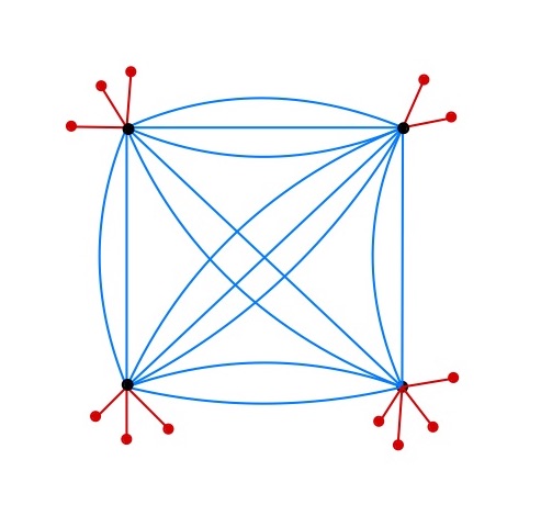
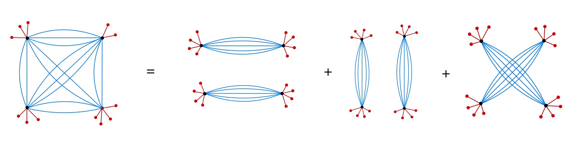
To get a general picture, we first compute $\langle z^{4}\rangle$ from the Feynman diagrams shown in Fig.8. In general it is a cumbersome combinatorial problem but in the large $N$ limit we know that it should be factorized into disconnected diagrams as

\displaystyle\langle z^{4}\rangle\approx 3{z_{2}^{(k)}}^{2}\,,\qquad\langle z^{2}\rangle\approx z_{2}^{(k)}\,,

(261)

which is shown in Fig.9 and here we have assumed that $z_{2}^{(k)}$ is the dominant wormhole saddles.

This means there are more refined structures of the nontrivial saddles in $z^{2}$ , comparing with the general discussion in Saad:2021rcu . Inspired by our analysis of the single half-wormhole for $z$ , we insert another two copies of identities (4.1) in $z^{2}$

	$\displaystyle z^{2}=\int\text{d}\sigma_{w}\text{d}\sigma_{h_{L}}\text{d}\sigma_{h_{R}}\Psi(\sigma_{w},\sigma_{h_{L}},\sigma_{h_{L}})\hat{\Lambda}(\sigma_{w},\sigma_{h_{L}},\sigma_{h_{L}})\,,$		(262)
	$\displaystyle\Psi(\sigma_{w},\sigma_{h_{L}},\sigma_{h_{L}})=\Psi(\sigma_{w})\Psi(\sigma_{h_{L}})\Psi(\sigma_{h_{R}})\,,$		(263)
	$\displaystyle\hat{\Lambda}(\sigma_{w},\sigma_{h_{L}},\sigma_{h_{L}})=\int\text{d}^{2N}\psi\exp[\text{i}e^{-\frac{2\text{i}\pi}{q}}\sigma_{h_{L}}\sum_{i<j}\psi^{L}_{ij}+\text{i}e^{-\frac{2\text{i}\pi}{q}}\sigma_{h_{R}}\sum_{i<j}\psi^{R}_{ij}+\text{i}e^{\frac{\text{i}\pi}{q}}\sigma_{w}\psi_{i}^{L}\psi_{i}^{R}$
	$\displaystyle\qquad\qquad\qquad\qquad+\text{i}^{q/2}J_{A}(\psi_{A}^{L}+\psi_{A}^{R})-\text{i}^{q/2}u\sum_{A}(\psi_{A}^{L}+\psi_{A}^{R})-\text{i}^{q}t^{2}\psi_{A}^{L}\psi_{A}^{R}],$		(264)

where we have introduced three pairs of $G,\Sigma$ variables

\displaystyle G_{w}=\frac{1}{N}\psi_{i}^{L}\psi_{i}^{R},\quad G_{h_{L}}=\frac{1}{N}\sum_{i<j}\psi^{L}_{ij},\quad G_{h_{R}}=\frac{1}{N}\sum_{i<j}\psi^{R}_{ij},

(265)

and rotated the contour as before. As before, the function $\Psi$ is highly peaked around $\Psi(0,0,0)$ so we expect that there is a half-wormhole saddle point

\displaystyle\Lambda=\hat{\Lambda}(0,0,0)

\displaystyle=\sum^{\prime}_{A,B}\text{sgn}(A)\text{sgn}(B)\prod_{k=1}^{p}\left((J_{A_{k}}-J_{A_{k}}^{0})(J_{B_{k}}-J_{B_{k}}^{0})-\delta_{A_{k}B_{k}}t^{2}\right)\,,

(266)

whose average manifestly vanishes $\langle\Lambda\rangle=0$ and it further satisfies $\langle\Lambda^{2}\rangle=2{z_{2}^{(p)}}^{2}$ .

However because of the large $N$ behavior (261), again we have to consider the fluctuations of $\sigma_{h}$ . It is achieved by expand $\hat{\Lambda}(0,\sigma_{h_{L}},\sigma_{h_{R}})$ with respect to $\sigma_{h_{L(R)}}$ or equivalently by expanding

\displaystyle\sum^{\prime}_{A,B}\text{sgn}(A)\text{sgn}(B)\prod_{k=1}^{p}\left((u+J_{A_{k}}-J_{A_{k}}^{0})(u+J_{B_{k}}-J_{B_{k}}^{0})-\delta_{A_{k}B_{k}}t^{2}\right)\equiv\sum_{n=0}^{p}\Lambda^{(k)}.

(267)

Some examples are

	$\displaystyle\Lambda^{(p-1)}=\sum_{i}\sum^{\prime}_{A,B}\text{sgn}(A)\text{sgn}(B)\left((J_{A_{1}}-J_{A_{1}}^{0})(J_{B_{1}}-J_{B_{1}}^{0})-\delta_{A_{1}B_{1}}t^{2}\right)\dots$
	$\displaystyle J_{A_{i}}^{0}J_{B_{i}}^{0}\dots\left((J_{A_{p}}-J_{A_{p}}^{0})(J_{B_{p}}-J_{B_{p}}^{0})-\delta_{A_{p}B_{p}}t^{2}\right),\quad\Lambda^{(0)}=\langle z\rangle^{2},\quad\Lambda^{(p)}=\Lambda\ .$

Then similarly one can find that

\displaystyle\langle\Lambda^{(k)}\Lambda^{(k)}\rangle=\langle z\Lambda^{(k)}\rangle=2{z_{2}^{(k)}}^{2}

(268)

so that when $z_{2}^{(k)}$ is the dominant wormhole saddle in the large $N$ limit the

\displaystyle z^{2}\approx\langle z^{2}\rangle+\Lambda^{(k)}\approx z_{2}^{(k)}+\Lambda^{(k)}\,,

(269)

is a good approximation.

5 SYK at one time point: $\langle J_{a}\rangle=0,\quad\langle J_{a}^{4}\rangle_{c}\neq 0$

Another class of interesting distributions of the random coupling is non-Gaussian. In this section we consider a special subset of them that have vanishing mean values, namely

\displaystyle\langle J_{A}\rangle=0\,,\qquad\langle J_{A}^{2}\rangle=t^{2}\,,\qquad\langle J_{A}^{4}\rangle=v^{4}+3\langle J_{A}^{2}\rangle^{2}\ .

(270)

It is easy to compute that the partition function of the 0d SYK model with such random couplings are

\displaystyle\langle z\rangle=0,\quad\langle z^{2}\rangle=\frac{N!}{p!(q!)^{p}}t^{2},\ .

(271)

The higher moments of $J_{A}$ in (6) contributes nontrivially to $\langle z^{4}\rangle$

\displaystyle\langle z^{4}\rangle

\displaystyle=

\displaystyle\sum_{A,B,C,D}^{\prime}\text{sgn}(A)\text{sgn}(B)\text{sgn}(C)\text{sgn}(D)\langle J_{A_{1}}J_{B_{1}}J_{C_{1}}J_{D_{1}}\dots J_{A_{p}}J_{B_{p}}J_{C_{p}}J_{D_{p}}\rangle\,,

(272)

which can be expanded

	$\displaystyle\langle z^{4}\rangle=\sum_{k=0}^{p}c_{k}n_{N-qk}v^{4k}t^{4(p-k)}\equiv\sum_{k}z_{4}^{(k)},$
	$\displaystyle n_{N}=\frac{N!}{(q!)^{2N/q}}\sum_{\begin{subarray}{c}n_{1}+n_{2}+n_{3}=N/q\\ n_{i}\geq 0\end{subarray}}\frac{(qn_{1})!(qn_{2})!(qn_{3})!}{(n_{1}!n_{2}!n_{3}!)^{2}},$
	$\displaystyle c_{k}n_{N-qk}=\frac{N!}{k!(q!)^{2p-k}}\sum_{\begin{subarray}{c}n_{1}+n_{2}+n_{3}=N/q-k\\ n_{i}\geq 0\end{subarray}}\frac{(qn_{1})!(qn_{2})!(qn_{3})!}{(n_{1}!n_{2}!n_{3}!)^{2}}$		(273)

where $c_{k}$ is the number of ways to choose $k$ $q$ -subsets out of $N$ and $n_{N}$ is the multiplicities coming from the different Wick contractions, i.e.

\displaystyle\langle z^{4}\rangle_{v=0}=n_{N}t^{4p}.

(274)

To find the dominant term in the large $N$ limit let us define the ratio

	$\displaystyle\tilde{r}_{k}=\frac{z_{4}^{(k)}}{z_{4}^{(k-1)}}\sim\frac{v^{4}}{t^{4}}\frac{1-k+p}{k}\frac{4!(4p-kp)!}{(4p-4k+4)!},$		(275)
	$\displaystyle\tilde{r}_{1}\sim\frac{v^{4}}{t^{4}}\frac{1}{p^{2}},\quad\tilde{r}_{p}\sim\frac{\upsilon^{4}}{t^{4}}\frac{1}{p}\,,$		(276)

where we have taken $q=4$ for simplicity. By taking the derivative with respect to $k$ we find that $\tilde{r}_{k}$ will initially decrease and then increase with increasing $k$ so $\tilde{r}_{p}$ is the maximal value. If $\tilde{r}_{p}\leq 1$ i.e.

\displaystyle\frac{v^{4}}{t^{4}}\leq p\,,

(277)

then the dominant term will be $z_{4}^{(0)}$ therefore the contributions of higher moments can be ignored in this limit. Recall that the half-wormhole saddle of $z^{2}$ when $\langle J_{A}\rangle=0$ can be written as

\displaystyle\Phi=\sum^{\prime}_{A,B}\text{sgn}(A)\text{sgn}(B)\left(J_{A_{1}}J_{B_{1}}-\delta_{A_{1}B_{1}}t^{2}\right)\dots\left(J_{A_{p}}J_{B_{p}}-\delta_{A_{p}B_{p}}t^{2}\right)\,,

(278)

such that

\displaystyle\langle\Phi^{2}\rangle\approx\langle\Phi z^{2}\rangle\approx 2\langle z^{2}\rangle^{2},

(279)

and

	$\displaystyle\langle\text{Error}^{2}\rangle$	$\displaystyle=$	$\displaystyle\langle z^{4}\rangle-\langle z^{2}\rangle^{2}+\langle\Phi^{2}\rangle-2\langle z^{2}\Phi^{2}\rangle$		(280)
		$\displaystyle\approx$	$\displaystyle 3\langle z^{2}\rangle^{2}-\langle z^{2}\rangle^{2}+2\langle z^{2}\rangle^{2}-4\langle z^{2}\rangle^{2}=0,$		(280)

in the leading order of $N$ as before. However if $\tilde{r}_{p}>1$ , then it will be possible that $z_{4}^{(p)}$ is the leading term whose corresponding Feynman diagram is shown in Fig.10.

Therefore there will be no half-wormhole saddle anymore since the (two-mouth) wormhole saddles are not dominant.

One can consider more general distribution with all the cumulants to be non-vanishing. The analysis and the results will be similar. If $v$ is very large then it is the four-way wormhole saddle that dominate. It is therefore possible to introduce a new ”four-linked-wormhole” saddle as we show in next section. However, if $v$ is relatively small it is still the two-mouth wormhole (with some legs as shown in Fig.7) that dominates. We will present a more thorough analysis of these points separately.

6 SYK at one time point: $\langle J_{a}\rangle=\langle J_{a}^{2}\rangle=\langle J_{a}^{3}\rangle=0$

In this section, we consider a special model where we could focus on the “multi-linked” wormhole saddle points. In this model the random coupling only have non-vanishing $4^{\text{th}}$ cumulant

\displaystyle\langle J_{a}\rangle=\langle J_{a}^{2}\rangle=\langle J_{a}^{3}\rangle=0,\quad\langle J_{a}^{4}\rangle=v^{4}\ .

(281)

Such a distribution could also be considered as an extremal limit of other distributions.

6.1 Averaged quantities: $\langle z^{4}\rangle$ and $\langle z^{8}\rangle$

Due to our special choice (281) the first non-vanishing averaged quantity is

	$\displaystyle\langle z^{4}\rangle$	$\displaystyle=$	$\displaystyle\int\text{d}^{4N}\psi\exp\left(v^{4}\sum_{A_{1}<\dots<A_{q}}\psi_{A_{1}}^{1}\psi_{A_{1}}^{2}\psi_{A_{1}}^{3}\psi_{A_{1}}^{4}\dots\psi_{A_{q}}^{1}\psi_{A_{q}}^{2}\psi_{A_{q}}^{3}\psi_{A_{q}}^{4}\right)$		(282)
		$\displaystyle=$	$\displaystyle\int\text{d}^{4N}\psi\exp\left(\frac{v^{4}}{q!}(\sum_{i}^{N}\psi_{i}^{1}\psi_{i}^{2}\psi_{i}^{3}\psi_{i}^{4})^{q}\right)\,.$		(282)

Then we can introduce the $G,\Sigma$ trick

$\displaystyle\langle z^{4}\rangle$	$\displaystyle=$	$\displaystyle\int\text{d}^{4N}\psi\int\text{d}G\,\delta(G_{4}-\sum_{i}^{N}\psi_{i}^{1}\psi_{i}^{2}\psi_{i}^{3}\psi_{i}^{4})\exp\left(\frac{v^{4}}{q!}G_{4}^{q}\right)$	(283)
	$\displaystyle=$	$\displaystyle\int\text{d}^{4N}\psi\int\text{d}G\frac{\text{d}\Sigma}{2\pi\text{i}}\exp\left(-\Sigma(G_{4}-\sum_{i}^{N}\psi_{i}^{1}\psi_{i}^{2}\psi_{i}^{3}\psi_{i}^{4})\right)\exp\left(\frac{v^{4}}{q!}G_{4}^{q}\right)$
	$\displaystyle=$	$\displaystyle\int\text{d}G\int\frac{\text{d}\Sigma}{2\pi\text{i}}\exp\left(N\log\Sigma-\Sigma G_{4}+\frac{v^{4}}{q!}G^{q}\right)$
	$\displaystyle=$	$\displaystyle(\partial_{G_{4}})^{N}\exp\left(\frac{\upsilon^{4}}{q!}G_{4}^{q}\right)\,\|_{G_{4}=0}=\left(\frac{v^{4}}{q!}\right)^{N/q}\frac{N!}{(N/q)!}=v^{4p}\frac{N!}{p!(q!)^{p}}\,.$

Alternatively, we can obtain this result by integrating out the fermions first to get the hyperpfaffin, taking the $4^{\text{th}}$ power, and then do the average

\displaystyle\langle z^{4}\rangle=\sum_{ABCD}\text{sgn}(A,B,C,D)\langle J_{A_{1}}J_{B_{1}}J_{C_{1}}J_{D_{1}}\dots J_{A_{p}}J_{B_{p}}J_{C_{p}}J_{D_{p}}\rangle=v^{4p}\sum_{A}\,1=v^{4p}\frac{N!}{p!(q!)^{p}}\,.

(284)

The computation of $\langle z^{8}\rangle$ is more involved

\displaystyle\langle z^{8}\rangle=\int\text{d}^{8N}\psi\exp\left(\frac{v^{4}}{q!}(\sum_{i}^{N}\psi_{i}^{a}\psi_{i}^{b}\psi_{i}^{c}\psi_{i}^{d})^{q}\right)\,,

(285)

where

\displaystyle(a,b,c,d)\in\{1\leq a<b<c<d\leq 8\}\ .

(286)

In the following we use the collective index $A^{\prime}$ to label the $4$ -element subset. Then we introduce antisymmetric tensors $G_{abcd}=G_{A^{\prime}}$ and $\Sigma_{abcd}=\Sigma_{A^{\prime}}$ as the collective field variables such that (284) can be expressed as

$\displaystyle\langle z^{8}\rangle$	$\displaystyle=$	$\displaystyle\int\frac{\text{d}G_{A^{\prime}}\text{d}\Sigma_{A^{\prime}}}{(2\pi\text{i})^{70}}(\text{PF}(\Sigma_{A^{\prime}}))^{N}\exp\left(-\sum_{A^{\prime}}[\Sigma_{A^{\prime}}G_{A^{\prime}}+\frac{v^{4}}{q!}G_{A^{\prime}}^{q}]\right)$	(287)
	$\displaystyle=$	$\displaystyle\left(\sum^{\prime}_{A^{\prime}_{1}<A^{\prime}_{2}}\text{sgn}(A^{\prime})\partial_{G_{A^{\prime}_{1}}}\partial_{G_{A^{\prime}_{2}}}\right)^{N}\exp\left(\frac{v^{4}}{q!}G_{A^{\prime}}^{q}\right)\|_{G_{A^{\prime}}=0}$
	$\displaystyle\approx$	$\displaystyle\left(\frac{v^{4}}{q!}\right)^{\frac{2N}{q}}\frac{N!^{2}}{p!^{2}}\frac{1}{2}{8\choose 4}=35\left(\frac{v^{4}}{q!}\right)^{\frac{2N}{q}}\frac{N!^{2}}{p!^{2}}\,,$

where in the last line we have taken the large $N$ limit. In this limit we have

\displaystyle\langle z^{8}\rangle\approx 35\langle z^{4}\rangle^{2}\ .

(288)

6.2 The un-averaged $z^{4}$

Following similar ideas as in the previous sections, we insert a suitable identity to the expression of $z^{4}$

\displaystyle z^{4}

\displaystyle=

\displaystyle\int\text{d}^{4N}\psi\exp\left(\text{i}^{q/2}\sum_{A,i}J_{A}\psi_{A}^{i}\right)\int\text{d}G_{4}\delta(G_{4}-\sum_{i}^{N}\prod_{a=1}^{4}\psi_{i}^{a})\exp\left(\frac{v^{4}}{q!}[G_{4}^{q}-(\sum_{i}^{N}\prod_{a=1}^{4}\psi_{i}^{a})^{q}]\right)\,

Rotating the contour as before we can rewrite $z^{4}$ as

\displaystyle z^{4}=\int\text{d}\sigma\Psi(\sigma)\hat{\Gamma}(\sigma)\,,

(290)

where $\Psi(\sigma)$ is same as (164) and the second factor is

\displaystyle\hat{\Gamma}(\sigma)=\int\text{d}^{4N}\psi\exp\left(\text{i}e^{-\frac{\text{i}\pi}{q}}\sigma\prod_{a}\psi^{a}_{i}+\text{i}^{q/2}\sum_{A,a}J_{A}\psi^{a}_{A}-v^{4}\sum_{A}\prod_{a}\psi_{A}^{a}\right).

(291)

Therefore we expect the half-wormhole saddle is given by

\displaystyle\Gamma=\hat{\Gamma}(0)

\displaystyle=

\displaystyle\sum_{ABCD}\text{sgn}(A,B,C,D)\prod_{k=1}^{p}(J_{A_{k}}J_{B_{k}}J_{C_{k}}J_{D_{k}}-\delta_{A_{k}}^{B_{k}}\delta_{C_{k}}^{B_{k}}\delta_{C_{k}}^{D_{k}}v^{4})\,,

(292)

which satisfies

	$\displaystyle\langle\Gamma\rangle=0\,,\qquad\langle\Gamma^{2}\rangle=\langle\Gamma z^{4}\rangle\approx 34\langle z^{4}\rangle^{2}\,,$		(293)
	$\displaystyle\langle(z^{4}-\langle z^{4}\rangle-\Gamma)^{2}\rangle=\langle z^{8}\rangle-\langle z^{4}\rangle^{2}+\langle\Gamma^{2}\rangle-2\langle\Gamma z^{4}\rangle\approx 0\,.$		(294)

We find clearly that the contribution from this four-linked-wormhole saddle is not equal to the square of (two-linked) half-wormhole saddle. Even though we derive it in the 0-SYK toy model, it should exist in other SYK-like theory as long as the $G,\Sigma$ trick can be applied. We will present some more details about these more general discussions somewhere else.

7 SYK at one time point: Poisson distribution

Up to now we have only considered random couplings with continuous probability distributions. It is also interesting to consider random couplings that take discrete values such as the Poisson distribution.

In fact the Poisson distribution, whose PDF and moments are given by (596) and (597), can be regarded as an opposite extremum to what we have considered above in the sense that all the cumulants are equal $\langle J^{n}\rangle_{c}=N\lambda$ , $\forall n$ . From the gravity point of view, it means that all the wormholes with different number of boundaries have the same amplitude. Ensemble theory or theories with random coupling with Poisson distribution have been studied in Marolf:2020xie ; Peng:2020rno ; Peng:2021vhs . If we view the index $i$ of $\psi^{i}$ as the label of different time points, then the effect of ensemble average is to introduce (“non-local”) interaction between different time points. In particular, starting with action (154) we can compute the first few moments¹¹¹¹11Here we have rescaled $q\rightarrow 2q$ , $N\rightarrow 2N$ .

$\displaystyle\langle z\rangle$	$\displaystyle=\int\text{d}^{2N}\psi\,e^{N\text{i}^{q}\lambda\sum_{A}\psi^{1}_{A}},$	(295)
$\displaystyle\langle z^{2}\rangle$	$\displaystyle=\int\text{d}^{4N}\psi\,e^{N\text{i}^{q}\lambda\sum_{A}(\psi_{A}^{1}+\psi_{A}^{2})}e^{N\text{i}^{2q}\lambda\sum_{A}\psi_{A}^{1}\psi_{A}^{2}},$	(296)
$\displaystyle\langle z^{3}\rangle$	$\displaystyle=\int\text{d}^{6N}\psi\,e^{N\text{i}^{q}\lambda\sum_{A}(\psi_{A}^{1}+\psi_{A}^{2}+\psi_{A}^{3})}e^{N\text{i}^{2q}\lambda\sum_{A}(\psi_{A}^{1}\psi_{A}^{2}+\psi_{A}^{1}\psi_{A}^{3}+\psi_{A}^{2}\psi_{A}^{3})}e^{N\text{i}^{3q}\lambda\sum_{A}\psi_{A}^{1}\psi_{A}^{2}\psi_{A}^{3}}\ .$	(297)

For a generic $k$ , we find

\displaystyle\langle z^{k}\rangle=\int\text{d}^{2kN}\psi e^{\lambda\sum_{A}\sum_{n=1}^{k}\frac{1}{n!}(\text{i}^{q}\sum^{k}_{i=1}(\psi_{A}^{i}))^{n}}\ .

(298)

Formally we can define

\displaystyle{\cal Z}(\lambda)\equiv\langle z^{\infty}\rangle=\int\text{d}\psi\exp\left\{N\lambda\sum_{A}(e^{\text{i}^{q}\sum_{i=1}\psi_{A}^{i}}-1)\right\}\,.

(299)

We can compute these moments by integrating out the fermions directly

\displaystyle\langle z^{n}\rangle=\langle\text{Pf}(J_{A})^{n}\rangle\ .

(300)

However the ensemble average of $\text{PF}(J_{A})^{n}$ is very complicated. Alternatively, if we only care about the large $N$ behavior we can use the $G,\Sigma$ trick and do a saddle point approximation. For example, the $G,\Sigma$ expression of $\langle z\rangle$ is similar to (215)

\displaystyle\langle z\rangle=\int d\Sigma dG(-\text{i})^{N}\Sigma^{N}e^{N\text{i}^{{q}}\lambda\frac{G^{{q}}}{{q}!}}e^{\text{i}N\Sigma G}.

(301)

The saddle point equations are

\displaystyle\Sigma G=\text{i},\quad\frac{\lambda}{(q-1)!}(\text{i}G)^{q}=1\,,

(302)

whose solutions are

\displaystyle\text{i}G=\left(\frac{(q-1)!}{\lambda}\right)^{1/q}e^{\frac{2m\pi\text{i}}{q}},\quad m=1,\dots,q\,.

(303)

It has been argued in Saad:2021rcu these $q$ saddle points should be added together to reproduce the correct large $N$ behavior in a very similar calculation. We expect the same to apply in the current situation¹²¹²12Here we have dropped the normalization factor $\text{i}^{N}$ .

\displaystyle\langle z\rangle_{\text{Disk}}=e^{-N(1-\frac{1}{q})}\left(\frac{N^{q}\lambda}{(q-1)!}\right)^{p}\sum_{m}e^{\frac{2m\pi\text{i}}{q}}=qe^{-N(1-\frac{1}{q})}\left(\frac{N^{q}\lambda}{(q-1)!}\right)^{p},

(304)

where $p=N/q$ as before. Adding the 1-loop factor $1/\sqrt{q}$ we end up with the correct large- $N$ behavior

\displaystyle\langle z\rangle_{\text{Disk}+1\text{ loop}}=\frac{1}{\sqrt{q}}e^{-N(1-\frac{1}{q})}\left(\frac{N^{q}\lambda}{(q-1)!}\right)^{p}.

(305)

Other moments can be computed similarly. For example, to compute $\langle z^{2}\rangle$ , we need to introduce three collective variables

\displaystyle G_{1}=\sum_{i<j}\text{i}\psi_{i}^{1}\psi_{j}^{1},\quad G_{2}=\sum_{i<j}\text{i}\psi_{i}^{2}\psi_{j}^{2},\quad G_{12}=\sum_{i}\psi_{i}^{1}\psi_{i}^{2}

(306)

such that

\displaystyle\text{i}^{q}\sum_{A}\psi_{A}^{1}=\frac{G_{1}^{q}}{q!},\quad\text{i}^{q}\sum_{A}\psi_{A}^{2}=\frac{G_{2}^{q}}{q!},\quad\text{i}^{2q}\sum_{A}\psi_{A}^{1}\psi_{A}^{2}=\frac{G_{12}^{2q}}{(2q)!}.

(307)

Imposing these relations with the help of a set of Lagrangian multiplier fields $\Sigma_{1}$ , $\Sigma_{2}$ and $\Sigma_{12}$ , the $\langle z^{2}\rangle$ can be expressed as

$\displaystyle\langle z^{2}\rangle$	$\displaystyle=$	$\displaystyle\int[\text{d}^{3}G_{i}d^{3}\Sigma_{i}]e^{N\frac{\lambda}{q!}(G_{1}^{q}+G_{2}^{q}+\frac{q!}{(2q)!}G_{12}^{2q})}e^{\text{i}N\sum_{i}(\Sigma_{i}G_{i})}\int\text{d}^{2N}\psi e^{\frac{1}{2}{\Psi}M{\Psi}},$	(308)
	$\displaystyle=$	$\displaystyle\int[\text{d}^{3}G_{i}d^{3}\Sigma_{i}]\sqrt{\text{det}[\Sigma_{1}\Sigma_{2}A^{2}-\Sigma_{12}^{2}I_{2N}]}e^{\frac{N\lambda}{q!}(G_{1}^{q}+G_{2}^{q}+\frac{q!}{(2q)!}G_{12}^{2q})}e^{\text{i}N\sum_{i}(\Sigma_{i}G_{i})}$	(309)
	$\displaystyle=$	$\displaystyle\int[\text{d}^{3}G_{i}d^{3}\Sigma_{i}]\text{i}^{2N}\text{det}[\sqrt{\Sigma_{1}\Sigma_{2}}A+\Sigma_{12}I_{N}]e^{N\frac{\lambda}{q!}(G_{1}^{q}+G_{2}^{q}+\frac{q!}{(2q)!}G_{12}^{2q})}e^{\text{i}N\sum_{i}(\Sigma_{i}G_{i})}$
	$\displaystyle=$	$\displaystyle\int[\text{d}^{3}G_{i}d^{3}\Sigma_{i}]\frac{\text{i}^{2N}}{2}\left((\Sigma_{12}+\sqrt{\Sigma_{1}\Sigma_{2}})^{2N}+(\Sigma_{12}-\sqrt{\Sigma_{1}\Sigma_{2}})^{2N}\right)e^{N\frac{N\lambda}{q!}(G_{1}^{q}+G_{2}^{q}+\frac{q!}{(2q)!}G_{12}^{2q})}e^{N\text{i}\sum_{i}(\Sigma_{i}G_{i})}$
	$\displaystyle=$	$\displaystyle\int[\text{d}^{3}G_{i}d^{3}\Sigma_{i}]\text{i}^{2N}\sum_{k=1}^{N}{2N\choose 2k}\Sigma_{12}^{2N-2k}(\Sigma_{1}\Sigma_{2})^{k}e^{N\frac{\lambda}{q!}(G_{1}^{q}+G_{2}^{q}+\frac{q!}{(2q)!}G_{12}^{2q})}e^{N\text{i}\sum_{i}(\Sigma_{i}G_{i})}$	(311)

where we have defined

	$\displaystyle\Psi=\left(\psi_{1}^{1},\dots,\psi_{2N}^{1},\psi_{1}^{2},\dots,\psi_{2N}^{2}\right),\quad M=\begin{pmatrix}\Sigma_{1}A&-\text{i}\Sigma_{12}I_{2N}\\ \text{i}\Sigma_{12}I_{2N}&\Sigma_{2}A\\ \end{pmatrix},$		(312)
	$\displaystyle A=-A^{T},\quad A_{ij}=1,\quad\forall i<j.$		(313)

The saddle point equations lead to

	$\displaystyle\text{i}\Sigma_{i}+\frac{\lambda}{(q-1)!}G_{i}^{q-1}=0,\quad i=1,2,$		(314)
	$\displaystyle\text{i}\Sigma_{12}+\frac{\lambda}{(2q-1)!}G_{12}^{2q-1}=0\,,\quad\sum_{i}\Sigma_{i}G_{i}=2\text{i}\ .$		(315)

This set of equations have multiple solutions. For example, the wormhole saddle is

	$\displaystyle G_{1}=G_{2}=\Sigma_{1}=\Sigma_{2}=0,\quad G_{12}=\left(\frac{2(2q-1)!}{\lambda}\right)^{1/2q}e^{\frac{2m\pi\text{i}}{2q}},$		(316)
	$\displaystyle\langle z^{2}\rangle_{WH+1\text{loop}}=\frac{1}{\sqrt{2q}}e^{-2N(1-\frac{1}{2q})}\left(\frac{(2N)^{2q}\lambda}{2(2q-1)!}\right)^{p}$		(317)

and the disconnected saddle is

	$\displaystyle G_{12}=\Sigma_{12}=0,\quad G_{1}=G_{2}=\left(\frac{(q-1)!}{\lambda}\right)^{1/q},$		(318)
	$\displaystyle\langle z^{2}\rangle_{disc+1\text{loop}}=\frac{1}{q}e^{-2N(1-\frac{1}{q})}\left(\frac{N^{q}\lambda}{(q-1)!}\right)^{2p}=\langle z\rangle_{\text{Disk}+1\text{loop}}^{2}.$		(319)

The ratio of these two saddles is

\displaystyle\frac{\langle z^{2}\rangle_{WH+1\text{loop}}}{\langle z^{2}\rangle_{disc+1\text{loop}}}=\sqrt{\frac{q}{2}}\left(\frac{q!^{2}2^{2q}}{e\lambda q(2q)!}\right)^{p}\,.

(320)

In the large $N$ or $p=N/q$ limit, the wormhole saddle can dominate only when $\lambda<\frac{q!^{2}2^{2q}}{e\lambda q(2q)!}\left(\frac{q}{2}\right)^{\frac{1}{2p}}$ which is consistent with our previous results.

Then a natural question is that in this limit how about other n-boundary wormhole saddles? In the following let us focus on a particular $n$ -linked-wormhole saddles. When $n=2k$ is even, the situation is similar to the one in section 6:

	$\displaystyle\langle z^{2k}\rangle_{\text{connected}}$	$\displaystyle=$	$\displaystyle\int d^{4kN}\psi\text{d}G\frac{\text{d}\Sigma}{2\pi}\exp\left(\text{i}N\Sigma\left(G-\sum_{i}^{2N}\prod_{a=1}^{2k}\psi_{i}^{a}\right)\right)\exp\left(N\frac{\lambda}{(2q)!}G^{2q}\right)$		(321)
		$\displaystyle=$	$\displaystyle\int\text{d}G\frac{\text{d}\Sigma}{2\pi}(\text{i}\Sigma)^{2N}\exp\left(\frac{N\lambda}{{(2q)}!}G^{2q}+\text{i}N\Sigma G\right)\,,$		(322)

where the collective variable $G$ is

\displaystyle G=\sum_{i}^{2N}\prod_{a=1}^{2k}\psi_{i}^{a}\ .

(323)

The expression (322) is of the same form as (301) so the saddle point approximation is

\displaystyle\langle z^{2k}\rangle_{2k-WH+1\text{loop}}=\langle z^{2}\rangle_{2-WH+1\text{loop}}=\frac{1}{\sqrt{2q}}e^{-2N(1-\frac{1}{2q})}\left(\frac{(2N)^{2q}\lambda}{2(2q-1)!}\right)^{p}.

(324)

When $n=2k+1$ is odd, the situation is similar to the one of $n=1$ :

	$\displaystyle\langle z^{2k+1}\rangle_{\text{connected}}$	$\displaystyle=$	$\displaystyle\int d^{(4k+2)N}\psi\text{d}G\frac{\text{d}\Sigma}{2\pi}\exp\left(\text{i}N\Sigma(G-\sum_{i<j}^{2N}\prod_{a=1}^{2k+1}\psi_{i}^{a}\prod_{a=1}^{2k+1}\psi_{j}^{a}\right)\exp\left(\frac{N\lambda}{q!}G^{q}\right)$		(325)
		$\displaystyle=$	$\displaystyle\int\text{d}G\frac{\text{d}\Sigma}{2\pi}(\text{i}\Sigma)^{2N}\exp\left(\frac{N\lambda}{{q}!}G^{q}+\text{i}N\Sigma G\right),$		(325)

where the collective variable $G$ is obviously defined as

\displaystyle G=\sum_{i<j}^{2N}\prod_{a=1}^{2k+1}\psi_{i}^{a}\prod_{a=1}^{2k+1}\psi_{j}^{a},

(326)

therefore the saddle point approximation is

\displaystyle\langle z^{2k+1}\rangle_{2k+1-HW+1\text{loop}}=\langle z\rangle_{\text{Disk}+1\text{loop}}=\frac{1}{\sqrt{q}}e^{-N(1-\frac{1}{q})}\left(\frac{N^{q}\lambda}{(q-1)!}\right)^{p}\ .

(327)

These higher $n$ -linked-wormholes should be compared with the corresponding powers of the disk solution, and furthermore since $\langle z^{2}\rangle_{2-WH+1\text{loop}}\gg 1$ , we conclude that all these multiple-linked-wormholes are suppressed. In other words, the ensemble of $z$ can be approximated by a Gaussian when the ratio (320) is of order 1.

8 The Brownian SYK model

In this section, we study the wormhole and half-wormholes saddles in the Brownian SYK model Saad:2018bqo . In the Brownian SYK model, the couplings are only correlated at the same instant of time so that after integrating over the coupling we end up with a local effective action¹³¹³13See Appendix (F) for general discussion on averaged model.. The quantity that is analogous to the partition function but with some information of real time evolution is

\displaystyle U(T)=\mathbf{T}e^{-\text{i}\int_{0}^{T}dtH(t)}\ .

(328)

To check the nature of its fluctuations that is not caused by the phase factor, we consider the norm square of its trace

\displaystyle\left|{\rm Tr}\,U(T)\right|^{2}\ .

(329)

This quantity is manifest real in the sense the complex conjugate maps ${\rm Tr}\,U(T)$ to ${\rm Tr}\,U(T)^{*}$ . The trace is over the Hilbert space, which has a path integral interpretation

\displaystyle{\rm Tr}\,U(T)

\displaystyle=\int\mathcal{D}\psi_{a}\exp\left\{-\text{i}\int_{0}^{T}dt\left[-\frac{\text{i}}{2}\psi_{a}\partial_{t}\psi_{a}+J_{a_{1}\ldots a_{q}}(t)\text{i}^{\frac{q}{2}}\psi_{a_{1}\ldots a_{q}}\right]\right\}\,,

(330)

where the Lagrangian density is manifestly real.

To compute (329), we introduce two replicas of fermions; $\psi^{(L)}$ constitute the fermions in $H$ of $U$ and $\psi^{(R)}$ in $U^{*}$ . Therefore the complex conjugate should map between $\psi^{(L)}$ and $\psi^{(R)}$ . One conventional way to define $\psi^{(R)}$ from $\psi^{(L)}$ is

\displaystyle\psi^{(R)}_{a}=\left(\psi^{(L)}_{a}\right)^{*}\ .

(331)

Then the complex conjugation of (330) is

\displaystyle{\rm Tr}\,U(T)^{*}

\displaystyle=\int\mathcal{D}\psi_{a}^{(R)}\exp\left\{-\text{i}\int_{0}^{T}dt\left[\frac{\text{i}}{2}\psi^{(R)}_{a}\partial_{t}\psi^{(R)}_{a}-J_{a_{1}\ldots a_{q}}(t)\text{i}^{\frac{q}{2}}\psi^{(R)}_{a_{1}\ldots a_{q}}\right]\right\}\,,

(332)

We can further do a field redefinition $\psi^{(R)}\to\text{i}\psi^{(R)}$ so that the kinetic term has the “right” sign¹⁴¹⁴14Here we choose to absorb an extra $i^{N}$ phase factor into the definition of the path integral measure. There might be $N\bmod 4$ effects that we will discuss separately.

\displaystyle{\rm Tr}\,U(T)^{*}

\displaystyle=\int\mathcal{D}\psi_{a}^{(R)}e^{-\text{i}\int_{0}^{T}dt\left[-\frac{\text{i}}{2}\psi^{(R)}_{a}\partial_{t}\psi^{(R)}_{a}-J_{a_{1}\ldots a_{q}}(t)(-\text{i})^{\frac{q}{2}}\psi^{(R)}_{a_{1}\ldots a_{q}}\right]}\,,

(333)

Combining (330), with $\psi_{a}$ replaced by $\psi_{a}^{(L)}$ , and (333), the quantity we would like to compute is

\displaystyle|\operatorname{Tr}U(T)|^{2}=\int\mathcal{D}\psi_{a}^{(L)}\mathcal{D}\psi_{a}^{(R)}e^{\text{i}\int_{0}^{T}dt\left[\frac{\text{i}}{2}\psi_{a}^{(j)}\partial_{t}\psi_{a}^{(j)}-J_{a_{1}\ldots a_{q}}(t)\left(\text{i}^{\frac{q}{2}}\psi_{a_{1}\ldots a_{q}}^{(L)}-(-\text{i})^{\frac{q}{2}}\psi_{a_{1}\ldots a_{q}}^{(R)}\right)\right]}\ .

(334)

A side remark is that the complex conjugation is closely related to time reversal symmetry $\mathcal{T}$ , and also because $[\mathcal{T},H]=0$ , we expect ${\rm Tr}\,U(T)^{*}={\rm Tr}\,U(-T)$ . Indeed, we find

	$\displaystyle{\rm Tr}\,U(-T)=\int\mathcal{D}\psi_{a}^{(R)}\exp\left\{-\text{i}\int_{0}^{-T}dt\left[-\frac{\text{i}}{2}\psi^{(R)}_{a}\partial_{t}\psi^{(R)}_{a}+J_{a_{1}\ldots a_{q}}(t)\text{i}^{\frac{q}{2}}\psi^{(R)}_{a_{1}\ldots a_{q}}\right]\right\}$		(335)
	$\displaystyle=\int\mathcal{D}\psi_{a}^{(R)}\exp\left\{\text{i}\int_{-T}^{0}dt\left[-\frac{\text{i}}{2}\psi^{(R)}_{a}\partial_{t}\psi^{(R)}_{a}+J_{a_{1}\ldots a_{q}}(t)\text{i}^{\frac{q}{2}}\psi^{(R)}_{a_{1}\ldots a_{q}}\right]\right\}$		(336)
	$\displaystyle=\int\mathcal{D}\psi_{a}^{(R)}\exp\left\{\text{i}\int_{0}^{T}dt\left[-\frac{\text{i}}{2}\psi^{(R)}_{a}\partial_{t}\psi^{(R)}_{a}+J_{a_{1}\ldots a_{q}}(t)\text{i}^{\frac{q}{2}}\psi^{(R)}_{a_{1}\ldots a_{q}}\right]\right\}={\rm Tr}\,U(T)^{*}\,,$		(337)

where we simply use $\psi^{(R)}$ to represent a different set of fermions that will be integrated over in the path integral; in particular, we do not think of them as the complex conjugate of the $\psi^{(L)}$ . In the last line we assume the system to be invariant under time translation, and the last equality is clear from (332). Therefore the quantity we are interested can also be written as ${\rm Tr}\,U(T){\rm Tr}\,U(-T)$ .

Note that the random couplings satisfy

\displaystyle\langle J_{A}\rangle=0,\quad\langle J_{A}(t)J_{B}(t^{\prime})\rangle=\delta(t-t^{\prime})\delta_{AB}{\cal J}^{2},\quad{\cal J}^{2}=2J\frac{(q-1)!}{N^{q-1}},

(338)

and the our normalization of one-dimensional Majorana fermions is

\displaystyle\{\psi_{i},\psi_{j}\}=\delta_{ij}\ .

(339)

To simplify our notation, we simply denote $\left|{\rm Tr}\,U(T)\right|^{2}$ by $\langle|z|^{2}\rangle$ in the rest computation.

8.1 $\langle|z|^{2}\rangle$ in the Brownian SYK model: accurate evaluation

As argued in Saad:2018bqo , we focus on the time independent configurations. Therefore we can directly integrate out the fermions and averaging over the random coupling according to (338). In the large $N$ limit and for even $q$ this leads to

\displaystyle\langle|z|^{2}\rangle

\displaystyle=\int_{\mathbb{R}}\mathcal{D}G_{LR}\int_{i\mathbb{R}}\frac{\mathcal{D}\Sigma_{LR}}{2\pi i/(TN)}e^{N\left[\log\left(2\cos\frac{T\Sigma_{LR}}{2}\right)-\frac{2JT}{q2^{q}}+i^{q}\frac{2JT}{q}G^{q}_{LR}-2\frac{T}{2}\Sigma_{LR}G_{LR}\right]}\ .

(340)

The integration measure is normalized such that if we first to the $G$ integral then the $\Sigma$ integral, we get the result of free fermions $\langle|z|^{2}\rangle|_{J=0}=2^{N}$ . Notice that the $G_{ij}$ function defined above is real under the complex conjugation (331). Making use of the identity

\displaystyle\int_{\text{i}\mathbb{R}}\frac{d\Sigma}{2\pi i/(TN)}e^{-NT\Sigma(G-x)}=\delta(G-x)

(341)

we get

\displaystyle\langle|z|^{2}\rangle=e^{-\frac{JNT}{q2^{q-1}}}\sum_{k=0}^{N}{N\choose k}e^{\frac{JTN}{q2^{q-1}}(\frac{2k}{N}-1)^{q}}\equiv c_{e}\,.

(342)

In the large- $N$ ( and also large- $NT$ ) limit, the dominant contribution are determined from two factors: the combinatoric factor and the exponential. At early time $T\ll 0$ , contributions from the different exponential factors are roughly the same, so the dominant term is determined from the largest term in the combinatoric factor

\displaystyle{N\choose N/2}=\frac{N!}{\left((N/2)!\right)^{2}}\sim 2^{N}\sqrt{\frac{2}{\pi N}}\,,

(343)

which leads to the contribution

\displaystyle c_{s}=\sqrt{\frac{2}{\pi N}}2^{N}e^{-\frac{JTN}{q2^{q-1}}}\ .

(344)

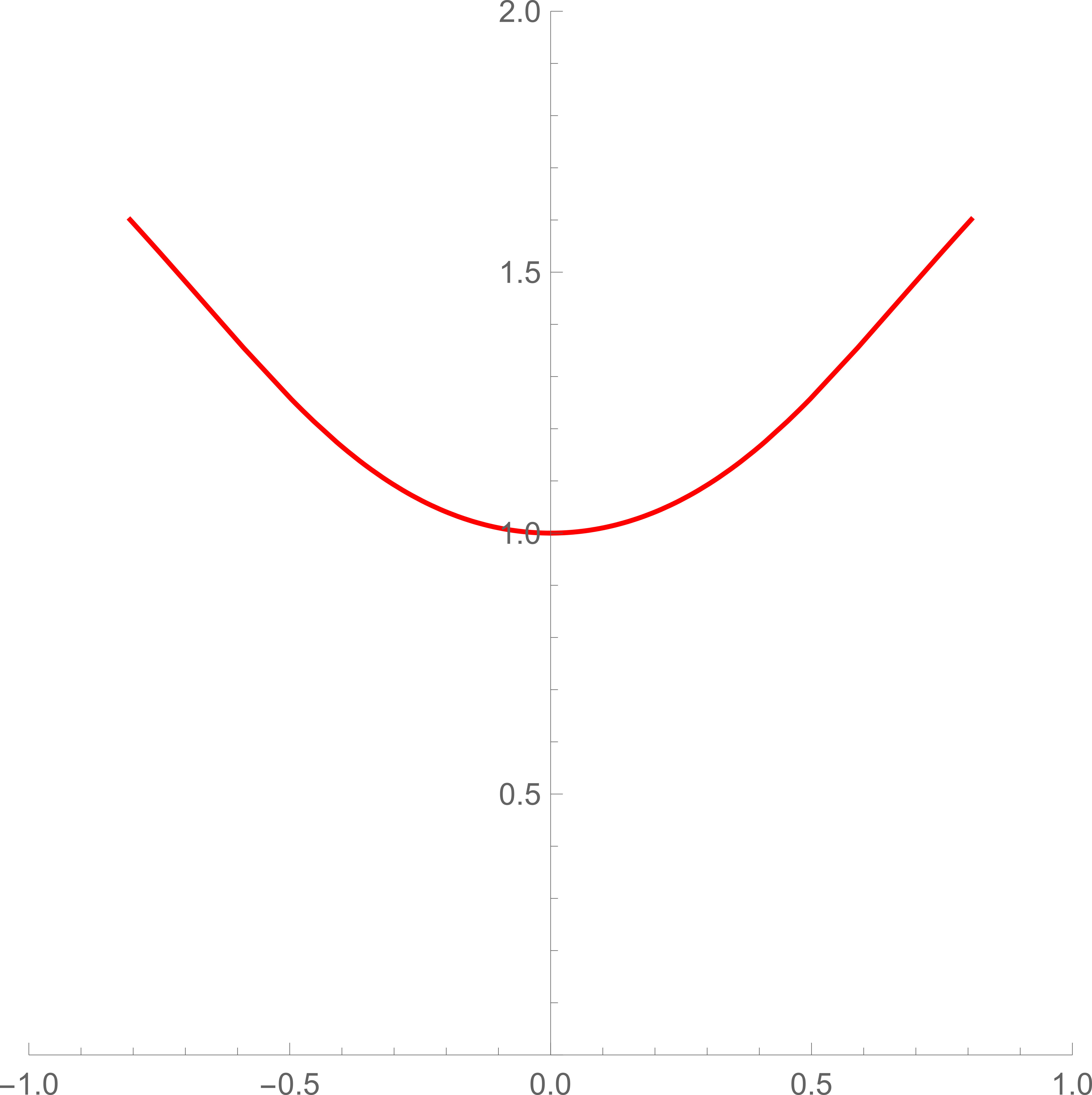
At late time, the different exponential factors dominant over the combinatoric factors, so the dominant contribution is from the maximal exponential factor, which is at $k=0,N$ with contributions to the sum being

\displaystyle c_{l}=2\ .

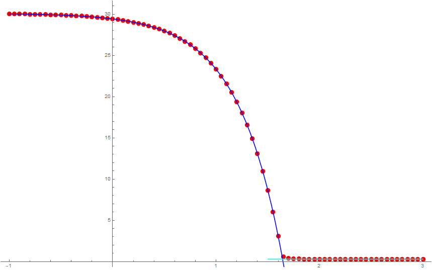
(345)

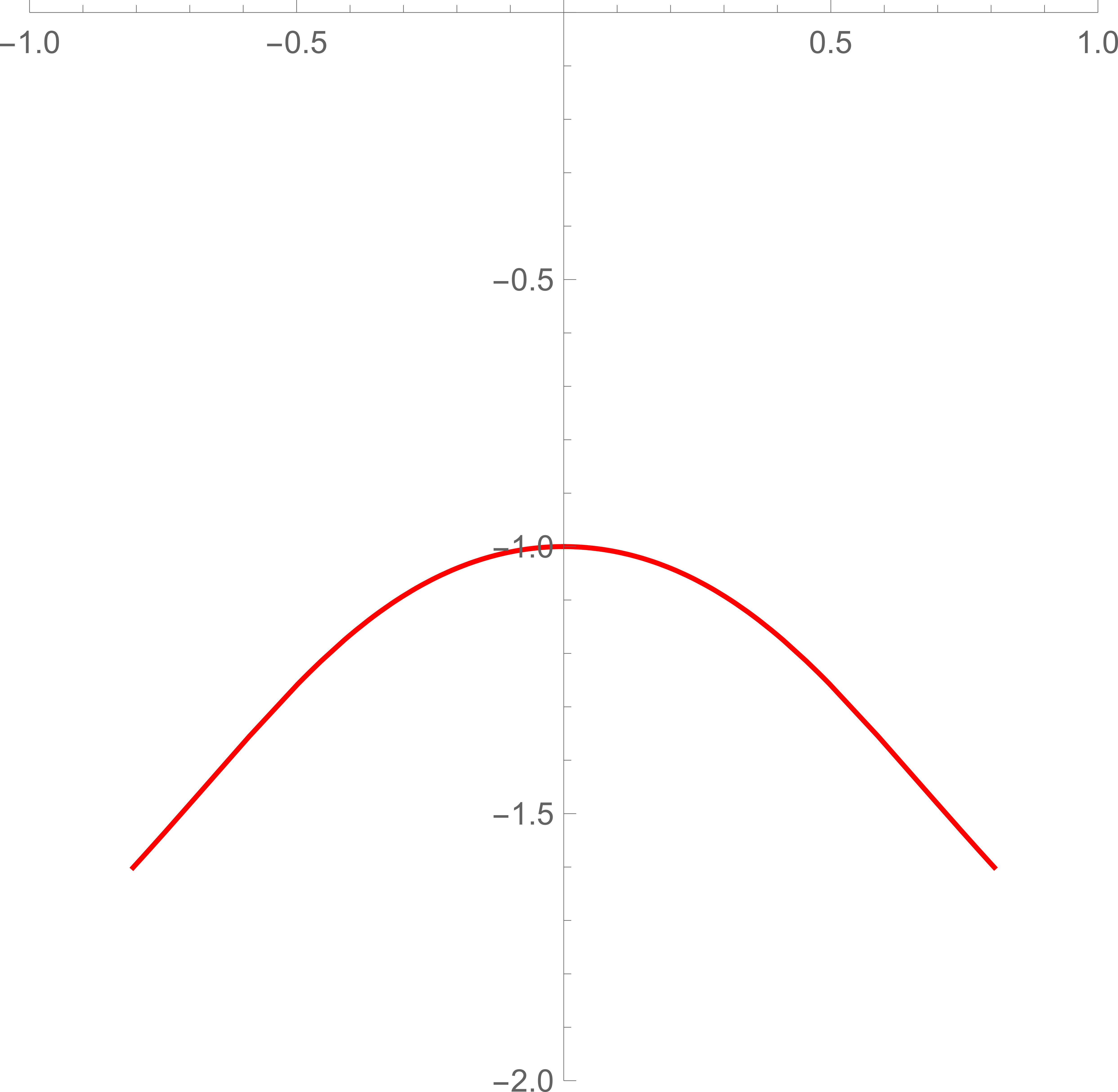
The behavior of $\langle|z|^{2}\rangle$ is shown in Figure. 11 where the early time exponential decay and the late time constant behavior is manifest.

8.2 $\langle|z|^{2}\rangle$ in the Brownian SYK model: large- $N$ saddle point evaluation

In the following, we perform a saddle point analysis to reproduce these distinct behaviors. We deform the integration contour together with a change of variable

\displaystyle G=\text{i}e^{\frac{\text{i}\pi}{q}}g,\quad\Sigma=e^{-\frac{\text{i}\pi}{q}}\sigma\ .

(346)

The action then reduces to

\displaystyle\langle|z|^{2}\rangle

\displaystyle=\int\mathcal{D}g\int\frac{\mathcal{D}\sigma_{LR}}{2\pi i/(TN)}e^{N\left[\log\left(2\cos\frac{Te^{-i\frac{\pi}{q}}\sigma}{2}\right)-\frac{2JT}{q2^{q}}-\frac{2JT}{q}g^{q}-Ti\sigma g\right]}\ .

(347)

The equation of motion of the $\sigma$ field leads to

\displaystyle g=\frac{\text{i}}{2}e^{-\frac{\text{i}\pi}{q}}\tan(\frac{T\sigma}{2}e^{-\frac{\text{i}\pi}{q}})\,,

(348)

while the equation of motion of $g$ is

\displaystyle\text{i}g\sigma+2Jg^{q}=0.

(349)

The two equations indicate a condition that $g$ should satisfy

\displaystyle g+\frac{1}{2}e^{-\frac{\text{i}\pi}{q}}\tanh({JT}g^{q-1}e^{-\frac{\text{i}\pi}{q}})=0\ .

(350)

Solutions to this equation are in general irrational. In the following we solve it with different approximations.

8.2.1 Saddle point solution: the $q=1$ case

Formally, we can consider the $q=1$ case where the saddle point solution can be found explicitly. In particular, when $q=1$ , the saddle point equation (350) reduces to

\displaystyle g=-\frac{1}{2}\tanh\left({TJ}\right)\,,\qquad\sigma=\text{i}J\ .

(351)

The on-shell action (with the 1-loop correction) is then

\displaystyle\langle|z|^{2}\rangle

\displaystyle=e^{{-\frac{2JTN}{2}}}\left(e^{-{JT}}+e^{{JT}}\right)^{N}\,.

(352)

On the other hand, when $q=1$ , the summation expression (342) can be evaluated explicitly to

\displaystyle\langle|z|^{2}\rangle=e^{{-{2JTN}{}}}\left(e^{-{JT}}+e^{{JT}}\right)^{N}\ .

(353)

The exact result agrees with the above saddle point result.

8.2.2 Saddle point solution: $q>1$ at short time $T\sigma\ll 1$

In the saddle point approach, the effective action in the short time limit can be expanded into

\displaystyle S_{\text{2}}=N\left(2T\left(-\frac{Jg^{q}}{q}-\frac{ig\sigma}{2}\right)-\frac{1}{8}e^{-\frac{2i\pi}{q}}\sigma^{2}T^{2}-\frac{e^{-\frac{4i\pi}{q}}\sigma^{4}T^{4}}{192}+\mathcal{O}(T^{5})\right)\,,

(354)

where

\displaystyle S_{\text{2}}=S-N\log(2)+NT\frac{2J}{q2^{q}}\,,

(355)

is the part of the action that depends on the dynamical fields, in other words, the constant piece in $S$ has been factored out to define $S_{2}$ . Notice that although we have $T\ll 1$ in this limit, we still want the saddle point approximation to be good, this means we want $NT\gg 1$ .

Before going to the details, we first discuss the region where this is a valid perturbative analysis. In the above expansion, the only $g$ dependence is in the $\left(-\frac{\text{i}\sigma g}{2}-\frac{J}{q}g^{q}\right)$ term, which means the set of saddle point equations always contain the following equation

\displaystyle 2\text{i}Jg^{q-1}=\sigma\ .

(356)

This relation means the saddle point contribution to the on shell action has the general form

\displaystyle S_{\text{2}}=N\left(\frac{2\left(-\frac{i}{2}\right)^{\frac{q}{q-1}}(q-1)TJ^{\frac{1}{1-q}}\tilde{\sigma}^{\frac{q}{q-1}}}{q}-\frac{1}{8}e^{-\frac{2i\pi}{q}}\sigma^{2}T^{2}-\frac{e^{-\frac{4i\pi}{q}}\sigma^{4}T^{4}}{192}+\mathcal{O}(T^{3})\right)\ .

(357)

Next, we would like to make sure our expansion of the $\log$ term is valid, this requires

\displaystyle T\sigma<1\ .

(358)

The remaining terms could switch dominance depending on the value of $\sigma$ in the saddle point solution.

	short time:	$\displaystyle T\sigma^{\frac{q}{q-1}}>T^{2}\sigma^{2}>T^{4}\sigma^{4}\,,\quad\Leftrightarrow\quad 0<\sigma<T^{\frac{q-1}{2-q}}\,,$		(359)
	intermediate time:	$\displaystyle T^{2}\sigma^{2}>T\sigma^{\frac{q}{q-1}}>T^{4}\sigma^{4}\,,\quad\Leftrightarrow\quad T^{\frac{q-1}{2-q}}<\sigma<T^{\frac{3(-1+q)}{4-3q}}\ .$		(360)

In all these cases the saddle point equation (350) reduces to the approximate form

\displaystyle g=\text{i}e^{-\frac{2\text{i}\pi}{q}}\sigma T\,,\quad\sigma=\text{i}g^{q-1}J\,.

(361)

$\bullet$ Short time

In this case, the dominant term in the action is

\displaystyle S_{\text{2}}=2NT\left(-\frac{Jg^{q}}{q}-\frac{g\sigma}{2}\right)\approx 2N\left(-\frac{\left((-1)^{\frac{1}{q-1}}(q-1)\right)TJ^{\frac{1}{1-q}}\sigma^{\frac{q}{q-1}}}{q2^{\frac{q}{q-1}}}\right)\ .

(362)

The $\sigma T$ term in the saddle point equation (361) can be dropped and the only solution is

\displaystyle g=0\,,\qquad\sigma=0\,,

(363)

This gives the following saddle contribution to the on-shell action

\displaystyle{NT}\exp\left\{N\left[\log\left(2\right)-\frac{2JT}{q2^{q}}\right]\right\}=2^{N}e^{-\frac{JTN}{q2^{q-1}}}NT\ .

(364)

Next we need to consider the quadratic fluctuations around this saddle

\displaystyle g\to g+\delta g\,,\qquad\sigma\to\sigma+\delta\sigma\ .

(365)

This gives the 1-loop factor

\displaystyle\frac{1}{NT}\,,

(366)

Therefore this saddle point approximation gives

\displaystyle\langle|z|^{2}\rangle_{s+1\text{loop}}

\displaystyle=\exp\left\{N\left[\log\left(2\right)-\frac{JT}{q2^{q}}\right]\right\}=2^{N}e^{-\frac{JTN}{q2^{q-1}}}\ .

(367)

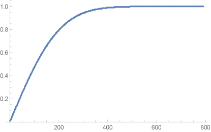
We next want to compare this saddle point approximation with the exact result (342). It is clear that in the small $T$ region the dominant saddle should be (344). However, it is also clear that the $k\sim\frac{N}{2}$ terms in the sum should also give comparable contributions. Indeed, if we compare the result (344) with (367), we find

\displaystyle\langle|z|^{2}\rangle_{s+1\text{loop}}=\sqrt{\frac{\pi N}{2}}c_{s}\ .

(368)

On the other hand, as we can check numerically,

\displaystyle c_{e}=\sqrt{\frac{\pi N}{2}}c_{s}\ ,\quad\text{when}\quad J\sim 1,\quad T\ll 1\ .

(369)

An example of this numerical check is shown in Figure. 12. Or we can understand this approximation as the following. When $J$ is of order 1 the exponent $e^{TN(1-\frac{2k}{N})^{q}}\leq e^{TN}$ . So if $T\sim\frac{1}{N}$ this exponent is always of order $1$ so that (342) can be approximated by $e^{-\frac{JNT}{q2^{q-1}}}\sum_{k}{N\choose k}=e^{-\frac{JNT}{q2^{q-1}}}2^{N}$ . Actually $T\sim 1/N$ is only a sufficient condition for (369) to hold; as can be observed from the numerical data $T$ can be much larger than $1/N$ .

Therefore, indeed we find our saddle point approximation agrees very well with the exact result.

$\bullet$ Intermediate time

In this region both the $\sigma^{2}$ and $\sigma^{\frac{q}{q-1}}$ terms in the action are roughly of the same order, so we need to solve the approximated saddle point equation (361). There are two solutions

\displaystyle\sigma=0\,,\qquad g=0\,,

(370)

and

\displaystyle g=\left(-e^{2\pi\text{i}m-\frac{2\text{i}\pi}{q}}\frac{JT}{2}\right)^{\frac{1}{2-q}}\,,\quad\sigma=2\text{i}Jg^{q-1}\ .

(371)

and both saddles should in principle be taken into account. Notice that the expression seems to blow up at $T\to 0$ , but we have fixed the range to be $\sim T_{0}$ so the expression remains finite. The saddle point contribution from the non-trivial solution (371) is proportional to

\displaystyle(NT)2^{N}e^{-\frac{2JNT}{q2^{q}}}\exp\left(\left(\frac{1}{2}-\frac{1}{q}\right)g^{q}\right)\,,

(372)

The loop correction around each of the saddle is

\displaystyle\frac{1}{NT\sqrt{q-2}}\ .

(373)

The full contribution is

\displaystyle 2^{N}e^{-\frac{2JNT}{q2^{q}}}\frac{1}{\sqrt{q-2}}\exp\left(N\frac{2-q}{2q}e^{\frac{2qm\text{i}\pi}{2-q}}\left(\frac{JT}{2}\right)^{\frac{2}{2-q}}\right)

(374)

However, it is easy to check numerically that the contributions to the on-shell action from these saddles (374) never dominate when $q>2$ . Therefore the trivial saddle point always has larger contribution and dominate the path integral in this range of time.

8.2.3 Long time $T\sigma\gg 1$

At long time, we can replace the $\cosh$ function by an exponential function. There are two choices, which leads to two different solutions

	$\displaystyle\log\left(2\cos(\frac{T\sigma}{2}e^{-\frac{\text{i}\pi}{q}})\right)$	$\displaystyle\sim\frac{\text{i}}{2}Te^{-\frac{\text{i}\pi}{q}}\sigma\,,\qquad\Re(\text{i}e^{-\text{i}\frac{\pi}{q}}\sigma)>0$		(375)
	$\displaystyle\log\left(2\cos(\frac{T\sigma}{2}e^{-\frac{\text{i}\pi}{q}})\right)$	$\displaystyle\sim-\frac{\text{i}}{2}Te^{-\frac{\text{i}\pi}{q}}\sigma\,,\qquad\Re(\text{i}e^{-\text{i}\frac{\pi}{q}}\sigma)<0\ .$		(376)

The solution of the saddle point equation in this case is time independent,

\displaystyle g=\pm\frac{1}{2}e^{-\frac{\text{i}\pi}{q}}\,,\sigma=2\text{i}Jg^{q-1}\ .

(377)

For even $q$ the on-shell actions of these saddles, including the 1-loop corrections, are also time independent

\displaystyle\langle|z|^{2}\rangle_{\text{WH}+1\text{1oop}}=2\times 1=2\,,

(378)

where the factor of 2 comes from adding up the contributions from the two saddles (377) and the result reproduces (345). In addition, the contribution from the trivial saddle vanishes at late time, so the non-trivial saddles (375) and (376) dominate. Since $g\neq 0$ , these saddle points are identified with wormhole saddles.

8.3 $\langle|z|^{4}\rangle$ in the Brownian SYK model

One of our goal in this section is to find possible half-wormhole saddles and study their relation to the wormhole saddle. To achieve this, it is helpful to first consider $|z|^{4}\equiv z_{1}z_{2}z_{3}z_{4}$ :

\displaystyle\int\mathcal{D}^{4N}\psi e^{\text{i}\int_{0}^{T}dt\left[\frac{\text{i}}{2}\psi_{a}^{(i)}\partial_{t}\psi_{a}^{(i)}-J_{a_{1}\ldots a_{q}}(t)\left(\text{i}^{\frac{q}{2}}\psi_{a_{1}\ldots a_{q}}^{(1)}-(-\text{i})^{\frac{q}{2}}\psi_{a_{1}\ldots a_{q}}^{(2)}+\text{i}^{\frac{q}{2}}\psi_{a_{1}\ldots a_{q}}^{(3)}-(-\text{i})^{\frac{q}{2}}\psi_{a_{1}\ldots a_{q}}^{(4)}\right)\right]}\,.

(379)

We first compute the ensemble averaged version $\langle z_{1}z_{2}z_{3}z_{4}\rangle$ :

$\displaystyle\langle\|z\|^{4}\rangle$	$\displaystyle=$	$\displaystyle\int{\cal D}^{4N}\psi\,e^{\int_{0}^{T}dt\left[-\frac{1}{2}\psi_{a}^{(i)}\partial_{t}\psi_{a}^{(i)}-\frac{{\cal J}^{2}}{2}\left(\text{i}^{\frac{q}{2}}\psi_{a_{1}\ldots a_{q}}^{(1)}-(-\text{i})^{\frac{q}{2}}\psi_{a_{1}\ldots a_{q}}^{(2)}+\text{i}^{\frac{q}{2}}\psi_{a_{1}\ldots a_{q}}^{(3)}-(-\text{i})^{\frac{q}{2}}\psi_{a_{1}\ldots a_{q}}^{(4)}\right)^{2}\right]}$	(380)
	$\displaystyle=$	$\displaystyle\int{\cal D}^{4N}\psi[\prod_{a<b}{\cal D}G_{ab}\frac{{\cal D}\Sigma_{ab}}{2\pi\text{i}/N}]\exp\left\{\int_{0}^{T}\text{d}t\left[-\frac{1}{2}\psi_{a}^{(i)}\partial_{t}\psi_{a}^{(i)}-\frac{4JNT}{q2^{q}}+\right.\right.$
		$\displaystyle\qquad\left.\left.2\sum_{a<b}\left(\frac{JN}{q}s_{ab}G_{ab}^{q}-N\frac{\Sigma_{ab}}{2}G_{ab}+\sum_{i}\frac{\Sigma_{ab}}{2}\psi_{i}^{a}\psi_{i}^{b}\right)\right]\right\}$

where $s_{12}=s_{14}=s_{23}=s_{34}=\text{i}^{q},\quad s_{13}=s_{24}=-1$ and the other orders of $(a,b)$ have been absorbed into the factor of 2. We again focus on the time-independent saddle points, and the integration over fermions gives

	$\displaystyle\int\text{d}^{4N}\psi\exp\left(\sum_{a<b}\Sigma_{ab}\psi_{i}^{a}\psi_{i}^{b}\right)$		(381)
	$\displaystyle\quad=2^{N}\left[\cos\left(\frac{1}{2}\sqrt{(\Sigma_{14}-\Sigma_{23})^{2}+(\Sigma_{13}+\Sigma_{24})^{2}+(\Sigma_{12}-\Sigma_{34})^{2}}\right)\right.$
	$\displaystyle\qquad\left.+\cos\left(\frac{1}{2}\sqrt{(\Sigma_{14}+\Sigma_{23})^{2}+(\Sigma_{13}-\Sigma_{24})^{2}+(\Sigma_{12}+\Sigma_{34})^{2}}\right)\right]^{N}\,,$		(382)

thus

	$\displaystyle\langle\|z\|^{4}\rangle$	$\displaystyle=\int[\prod_{a<b}{\cal D}G_{ab}\frac{{\cal D}\Sigma_{ab}}{2\pi\text{i}/(NT)}]e^{-\frac{4JNT}{q2^{q}}}\exp\left(S_{\text{eff}}\right)\,,$		(383)
	$\displaystyle S_{\text{eff}}$	$\displaystyle=2NT\sum_{a<b}\left(\frac{J}{q}s_{ab}G_{ab}^{q}-\frac{\Sigma_{ab}}{2}G_{ab}\right)+N\log(e^{\text{i}Tf_{+}}+e^{-\text{i}Tf_{+}}+e^{\text{i}Tf_{-}}+e^{-\text{i}Tf_{-}})\,,$		(384)

with

\displaystyle f_{\pm}=\frac{1}{2}\sqrt{(\Sigma_{14}\pm\Sigma_{23})^{2}+(\Sigma_{13}\mp\Sigma_{24})^{2}+(\Sigma_{12}\pm\Sigma_{34})^{2}}\ .

(385)

8.3.1 Exact evaluation

Similar to the exact calculation of $\langle|z|^{2}\rangle$ we can integrate $\Sigma_{AB}$ first to obtain

	$\displaystyle\langle\|z\|^{4}\rangle$	$\displaystyle=$	$\displaystyle e^{-\frac{4JNT}{q2^{q}}}\left(e^{\frac{\text{i}\hat{f}_{+}}{N}}+e^{-\frac{\text{i}\hat{f}_{+}}{N}}+e^{\frac{\text{i}\hat{f}_{-}}{N}}+e^{-\frac{\text{i}\hat{f}_{-}}{N}}\right)^{N}e^{\frac{2NTJ}{q}\sum_{a<b}s_{ab}G_{ab}^{q}}\,\Big{\|}_{G_{ab}=0}\,$		(386)
		$\displaystyle=$	$\displaystyle e^{-\frac{4JNT}{q2^{q}}}\sum_{0\leq n_{i}\leq N,\sum_{i}n_{i}=N}e^{\frac{\text{i}(n_{1}-n_{2})}{N}\hat{f}_{+}}e^{\frac{\text{i}(n_{3}-n_{4})}{N}\hat{f}_{-}}e^{\frac{2NTJ}{q}\sum_{a<b}s_{ab}G_{ab}^{q}}\,\Big{\|}_{G_{ab}=0}\,,$		(387)

where we have introduced the differential operators

\displaystyle\hat{f}_{\pm}=\frac{1}{2}\sqrt{(\partial_{G_{14}}\pm\partial_{G_{23}})^{2}+(\partial_{G_{13}}\mp\partial_{G_{24}})^{2}+(\partial_{G_{12}}\pm\partial_{G_{34}})^{2}}.

(388)

Expanding the exponentials into Taylor series and keeping only the non-vanishing terms we get

	$\displaystyle e^{\frac{\text{i}(n_{1}-n_{2})}{N}\hat{f}_{+}}e^{\frac{\text{i}(n_{3}-n_{4})}{N}\hat{f}_{-}}e^{\frac{2NTJ}{q}\sum_{a<b}s_{ab}G_{ab}^{q}}\,\Big{\|}_{G_{ab}=0},$
	$\displaystyle=\sum_{n=0}^{\infty}\sum_{m=0}^{\infty}\left(\frac{\text{i}(n_{1}-n_{2})}{N}\right)^{mq}\left(\frac{\text{i}(n_{3}-n_{4})}{N}\right)^{nq}\frac{\hat{f}_{+}^{mq}\hat{f}_{-}^{nq}}{(mq)!(nq)!}e^{\frac{2NTJ}{q}\sum_{a<b}s_{ab}G_{ab}^{q}}\,\Big{\|}_{G_{ab}=0}\,,$		(389)

with

	$\displaystyle\hat{f}_{+}^{mq}\hat{f}_{-}^{nq}$	$\displaystyle=\frac{1}{2^{(n+m)q}}\sum_{\begin{subarray}{c}0\leq k^{+}_{i}\leq m,\sum k_{i}^{+}=m\\ 0\leq k^{-}_{i}\leq n,\sum k^{-}_{i}=n\end{subarray}}\left((\partial_{G_{14}}+\partial_{G_{23}})^{k_{1}^{+}q}(\partial_{G_{14}}-\partial_{G_{23}})^{k_{1}^{-}q}\right.$
		$\displaystyle\times\left.(\partial_{G_{13}}-\partial_{G_{24}})^{k_{2}^{+}q}(\partial_{G_{13}}+\partial_{G_{24}})^{k_{2}^{-}q}(\partial_{G_{12}}+\partial_{G_{34}})^{k_{3}^{+}q}(\partial_{G_{12}}-\partial_{G_{34}})^{k_{3}^{-}q}\right)\,.$		(390)

For each pair of differential operators in (390) the contribution can be obtained for example as

	$\displaystyle(\partial_{G_{14}}+\partial_{G_{23}})^{k_{1}^{+}q}(\partial_{G_{14}}-\partial_{G_{23}})^{k_{1}^{-}q}e^{-\frac{2NTJ}{q}(G_{14}^{q}+G_{23}^{q})}\Big{\|}_{G_{ab}=0}$
	$\displaystyle=\sum_{l^{+}_{1}=0,l^{-}_{1}=0}^{k_{1}^{+},k_{1}^{-}}{k_{1}^{+}q\choose l_{1}^{+}q}{k_{1}^{-}q\choose l_{1}^{-}q}\partial_{G_{14}}^{(l_{1}^{+}+l_{1}^{-})q}\partial_{G_{23}}^{(k_{1}^{+}+k_{1}^{-}-l_{1}^{+}-l_{1}^{-})q}e^{\text{i}^{q}\frac{2NTJ}{q}(G_{14}^{q}+G_{23}^{q})}\Big{\|}_{G_{ab}=0}$		(391)
	$\displaystyle=\left(\text{i}^{q}\frac{2NJT}{q}\right)^{(k_{1}^{+}+k_{1}^{-})q}\sum_{l^{+}_{1}=0,l^{-}_{1}=0}^{k_{1}^{+},k_{1}^{-}}{k_{1}^{+}q\choose l_{1}^{+}q}{k_{1}^{-}q\choose l_{1}^{-}q}\frac{[(l_{1}^{+}+l_{1}^{-})q]![(k_{1}^{+}+k_{1}^{-}-l_{1}^{+}-l_{1}^{-})q]!}{(l_{1}^{+}+l_{1}^{-})!(k_{1}^{+}+k_{1}^{-}-l_{1}^{+}-l_{1}^{-})!}$
	$\displaystyle\equiv\left(\text{i}^{q}\frac{2NJT}{q}\right)^{(k_{1}^{+}+k_{1}^{-})q}\Delta(k_{1}^{+},k_{1}^{-}).$		(392)

Thus the full expression of (386) is

	$\displaystyle\langle\|z\|^{4}\rangle=e^{-\frac{4JNT}{q2^{q}}}\sum_{\begin{subarray}{c}0\leq n_{i}\leq N,\\ \sum_{i}n_{i}=N\end{subarray}}\sum_{n=0}^{\infty}\sum_{m=0}^{\infty}\sum_{\begin{subarray}{c}0\leq k^{+}_{i}\leq m,\sum k_{i}^{+}=m\\ 0\leq k^{-}_{i}\leq n,\sum k^{-}_{i}=n\end{subarray}}\sum_{l^{+}_{i}=0,l^{-}_{i}=0}^{k_{i}^{+},k_{i}^{-}}\frac{(\frac{\text{i}n_{12}}{N})^{mq}}{(mq)!2^{mq}}\frac{(\frac{\text{i}n_{34}}{N})^{nq}}{(nq)!2^{nq}}$
	$\displaystyle\quad\left(\text{i}^{q}\frac{2NJT}{q}\right)^{(k_{1}^{+}+k_{1}^{-}+k_{3}^{+}+k_{3}^{-})q}\left(-\frac{2NJT}{q}\right)^{(k_{2}^{+}+k_{2}^{-})q}\prod_{i=1}^{3}\Delta(k_{i}^{+},k_{i}^{-})\,,$		(393)

where $n_{12}=n_{1}-n_{2}$ and $n_{34}=n_{3}-n_{4}$ . This is very complicated expression but at large T and large $N$ , the leading contributions come from the cases when $n_{i}=N$ and $n_{j}=0,j\neq i$ . For each of these cases, we show in Appendix (D) that it contributes 2 when $q=4m$ and 3 when $q=4m+2$ . So in total, $\langle z_{4}\rangle_{T\rightarrow\infty}$ approaches to 8 when $q=4m$ and 12 when $q=4m+2$ .

Next we turn to the saddle point analysis and try to match the results.

8.3.2 Saddle point analysis

To make the integral (384) convergent, we do the following change of variables and deform the original integral contour so that the integral over $g_{ab}$ and $\sigma_{ab}$ are along the real lines

	$\displaystyle G_{12}=\text{i}e^{\frac{\text{i}\pi}{q}}g_{12},\quad G_{23}=\text{i}e^{\frac{\text{i}\pi}{q}}g_{23},\quad G_{14}=\text{i}e^{\frac{\text{i}\pi}{q}}g_{14},\quad G_{34}=\text{i}e^{\frac{\text{i}\pi}{q}}g_{34},$		(394)
	$\displaystyle\Sigma_{12}=e^{-\frac{\text{i}\pi}{q}}\sigma_{12},\quad\Sigma_{23}=e^{-\frac{\text{i}\pi}{q}}\sigma_{23},\quad\Sigma_{14}=e^{-\frac{\text{i}\pi}{q}}\sigma_{14},\quad\Sigma_{34}=e^{-\frac{\text{i}\pi}{q}}\sigma_{34},$		(395)
	$\displaystyle G_{13}=g_{13},\quad G_{24}=g_{24},\quad\Sigma_{13}=\text{i}\sigma_{13},\quad\Sigma_{24}=\text{i}\sigma_{24}\ .$		(396)

The effective action then becomes

\displaystyle S=2NT\sum_{ab}\left(-\frac{J}{q}g_{ab}^{q}-\text{i}\frac{\sigma_{ab}}{2}g_{ab}\right)+N\log(e^{\text{i}Tf_{+}}+e^{-\text{i}Tf_{+}}+e^{\text{i}Tf_{-}}+e^{-\text{i}Tf_{-}})\ .

(397)

Let us again focus on the large $T$ limit. In this limit, we expect only one of the four exponentials $e^{\pm\text{i}Tf_{\pm}}$ dominates the integral. To be explicit, let us assume the dominant one to be

\displaystyle e^{\text{i}a\frac{T}{2}\sqrt{(\Sigma_{14}+b\Sigma_{23})^{2}+(\Sigma_{13}-b\Sigma_{24})^{2}+(\Sigma_{12}+b\Sigma_{34})^{2}}}=e^{\text{i}a\frac{T}{2}\sqrt{e^{-\frac{2\text{i}\pi}{q}}(\sigma_{14}+b\sigma_{23})^{2}-(\sigma_{13}-b\sigma_{24})^{2}+e^{-\frac{2\text{i}\pi}{q}}(\sigma_{12}+b\sigma_{34})^{2}}}\,,

(398)

where $a,b$ can be $\pm 1$ . The saddle point equations leads to

\displaystyle g_{34}=bg_{12},\quad g_{24}=-bg_{13},\quad g_{23}=bg_{14},\quad\sigma_{ab}=2\text{i}Jg^{q-1}_{ab},\quad g_{12}^{2}e^{\frac{2\text{i}\pi}{q}}+g_{14}^{2}e^{\frac{2\text{i}\pi}{q}}-g_{13}^{2}=1\ .

(399)

There is always a trivial saddle solution

\displaystyle g_{ab}=\sigma_{ab}=0,\quad\langle|z|^{4}\rangle_{\text{trivial}}=2^{2N}e^{-\frac{JNT}{q2^{q-2}}}\,,

(400)

which corresponds to the disconnected topology.

There is in addition a large number of non-trivial saddle solutions. ones with largest contributions to the on-shell actions, including the 1-loop corrections, are

	$\displaystyle g_{12}=bg_{34}=a\frac{1}{2}e^{-\frac{\text{i}\pi}{q}},\quad g_{13}=g_{14}=g_{23}=g_{24}=0,\quad\langle\|z\|^{4}\rangle_{12}=1,$		(401)
	$\displaystyle g_{13}=-bg_{24}=a\frac{\text{i}}{2},\quad g_{12}=g_{14}=g_{23}=g_{34}=0,\quad\langle\|z\|^{4}\rangle_{13}=e^{-\frac{2(1+(\text{i})^{q})NJT}{q}},$		(402)
	$\displaystyle g_{14}=bg_{23}=a\frac{1}{2}e^{-\frac{\text{i}\pi}{q}},\quad g_{13}=g_{12}=g_{34}=g_{24}=0,\quad\langle\|z\|^{4}\rangle_{14}=1\,,$		(403)

where the last equation in each line is the on-shell action of the corresponding solution. Apparently (401) and (403) correspond to the wormhole saddles appearing in $\langle|z|^{2}\rangle$ and (402) correspond to the possible wormhole saddle appearing in $\langle z^{2}\rangle$ . Therefore we find that in the late time

\displaystyle\langle z^{4}\rangle_{WH}=\begin{cases}3\langle z^{2}\rangle^{2}_{WH}&q=4k+2,\\ 2\langle z^{2}\rangle^{2}_{WH}&q=4k.\end{cases}

(404)

Notice that for $a=\pm 1$ the real parts of $e^{iTf_{p}}$ and $e^{-iTf_{p}}$ are the same, so it is not possible that only the $a=1$ term dominate; what happens is that when the $e^{iaTf_{p}}$ dominates, the $e^{-iaTf_{p}}$ term also dominates and the resulting path integral result is just twice of the above results (401)-(403). Further taking into account that $b$ can be $\pm 1$ we find that total saddle point contributions are 8 when $q=4k$ and 12 when $q=4k+2$ as we found in the exact evaluation.

The interesting $q\bmod 4$ relation is consistent with the time reversal symmetry.

8.4 $z^{2}$ at fixed coupling in the Brownian SYK model

In the following we consider the non-average expression (334), which we recall here

\displaystyle|\operatorname{Tr}U(T)|^{2}=\int\mathcal{D}\psi_{a}^{(L)}\mathcal{D}\psi_{a}^{(R)}e^{\text{i}\int_{0}^{T}dt\left[\frac{\text{i}}{2}\psi_{a}^{(j)}\partial_{t}\psi_{a}^{(j)}-J_{a_{1}\ldots a_{q}}(t)\left(\text{i}^{\frac{q}{2}}\psi_{a_{1}\ldots a_{q}}^{(L)}-(-\text{i})^{\frac{q}{2}}\psi_{a_{1}\ldots a_{q}}^{(R)}\right)\right]}\ .

(405)

We can again introduce

\displaystyle 1=\int_{\mathbb{R}}\mathcal{D}G_{LR}\int_{\text{i}\mathbb{R}}\frac{\mathcal{D}\Sigma_{LR}}{2\times 2\pi\text{i}/N}e^{-\int\text{d}tdt^{\prime}{\frac{\Sigma_{LR}(t,t^{\prime})}{2}}\left(NG_{LR}(t,t^{\prime})-\sum_{a}\psi^{L}_{a}(t)\psi^{R}_{a}(t^{\prime})\right)}e^{f_{LR}\left(NG_{LR}\right)-f_{LR}\left(\sum_{a}\psi^{L}_{a}\psi^{R}_{a}\right)}\ .

(406)

The quantity we would like to compute is

$\displaystyle\|\operatorname{Tr}U(T)\|^{2}$	$\displaystyle=\int_{\mathbb{R}}\mathcal{D}G_{LR}\int_{\text{i}\mathbb{R}}\frac{\mathcal{D}\Sigma_{LR}}{2\times 2\pi\text{i}/N}\int\mathcal{D}\psi_{a}^{(L)}\mathcal{D}\psi_{a}^{(R)}$	(407)
	$\displaystyle\times\exp\left\{\text{i}\int_{0}^{T}dt\left[\frac{\text{i}}{2}\psi_{a}^{(j)}\partial_{t}\psi_{a}^{(j)}-J_{a_{1}\ldots a_{q}}(t)\left(\text{i}^{\frac{q}{2}}\psi_{a_{1}\ldots a_{q}}^{(L)}-(-\text{i})^{\frac{q}{2}}\psi_{a_{1}\ldots a_{q}}^{(R)}\right)\right]\right\}$	(408)
	$\displaystyle\times e^{-\int\text{d}t\text{d}t^{\prime}{\frac{\Sigma_{LR}(t,t^{\prime})}{2}}\left(NG_{LR}(t,t^{\prime})-\sum_{a}\psi^{L}_{a}(t)\psi^{R}_{a}(t^{\prime})\right)}e^{f_{LR}\left(NG_{LR}\right)-f_{LR}\left(\sum_{a}\psi^{L}_{a}\psi^{R}_{a}\right)}\ .$	(409)

We further rewrite

\displaystyle|\operatorname{Tr}U(T)|^{2}=\int_{\mathbb{R}}\frac{\mathcal{D}\Sigma_{LR}}{2\pi/N}\Phi(\Sigma_{LR})\Psi(\Sigma_{LR})\ .

(410)

The $\psi_{a}$ independent part reads

\displaystyle\Psi(\Sigma_{LR})=\int_{\mathbb{R}}\mathcal{D}G_{LR}e^{-\int\text{d}t\text{d}t^{\prime}N{\frac{\Sigma_{LR}(t,t^{\prime})}{2}}G_{LR}(t,t^{\prime})}e^{f_{LR}\left(NG_{LR}\right)}\,,

(411)

where

\displaystyle f_{LR}(NG_{LR})=\frac{2J}{N^{q-1}q}(-1)^{\frac{q}{2}}\left(NG_{LR,ii}\right)^{q}\ .

(412)

The $\psi_{a}$ dependent part is

	$\displaystyle\Phi(\Sigma_{LR})=$	$\displaystyle\int\mathcal{D}\psi_{a}^{(L)}\mathcal{D}\psi_{a}^{(R)}e^{\frac{1}{2}\int\text{d}t\text{d}t^{\prime}\Sigma_{LR}(t,t^{\prime})\left(\psi^{L}_{a}(t)\psi^{R}_{a}(t^{\prime})\right)-f_{LR}(\sum_{a}\psi^{L}_{a}\psi^{R}_{a})}$		(413)
		$\displaystyle\times\exp\left\{\text{i}\int_{0}^{T}dt\left[\frac{\text{i}}{2}\psi_{a}^{(j)}\partial_{t}\psi_{a}^{(j)}-J_{a_{1}\ldots a_{q}}(t)\left(\text{i}^{\frac{q}{2}}\psi_{a_{1}\ldots a_{q}}^{(L)}-(-\text{i})^{\frac{q}{2}}\psi_{a_{1}\ldots a_{q}}^{(R)}\right)\right]\right\}\ .$		(414)

For the integral over $G_{LR}$ to converge, we rotate the contour so that

\displaystyle\Sigma_{LR}=e^{-\text{i}\frac{\pi}{q}}\sigma\,,\quad G_{LR}=\text{i}e^{\text{i}\frac{\pi}{q}}g\ .

(415)

If we now compute the average of $\Phi(\sigma)$ , we get

$\displaystyle\langle\Phi(\sigma)\rangle$	$\displaystyle=\int\mathcal{D}\psi_{a}^{(L)}\mathcal{D}\psi_{a}^{(R)}e^{\frac{1}{2}\int\text{d}t\text{d}t^{\prime}\Sigma_{LR}(t,t^{\prime})\left(\psi^{L}_{a}(t)\psi^{R}_{a}(t^{\prime})\right)-f_{LR}(\sum_{a}\psi^{L}_{a}\psi^{R}_{a})}$	(416)
	$\displaystyle\times\exp\left\{\int_{0}^{T}\text{d}t\left[\frac{-1}{2}\psi_{a}^{(j)}\partial_{t}\psi_{a}^{(j)}-\frac{{\cal J}^{2}}{2}\left(\text{i}^{\frac{q}{2}}\psi_{a_{1}\ldots a_{q}}^{(L)}-(-\text{i})^{\frac{q}{2}}\psi_{a_{1}\ldots a_{q}}^{(R)}\right)^{2}\right]\right\}$	(417)
	$\displaystyle=\int\mathcal{D}\psi_{a}^{(L)}\mathcal{D}\psi_{a}^{(R)}e^{\frac{1}{2}\int dtdt^{\prime}\Sigma_{LR}(t,t^{\prime})\left(\psi^{L}_{a}(t)\psi^{R}_{a}(t^{\prime})\right)}e^{-\int_{0}^{T}dt\left[\frac{1}{2}\psi_{a}^{(j)}\partial_{t}\psi_{a}^{(j)}+\frac{{\cal J}^{2}}{2^{q}}{N\choose q}\right]}\ .$	(418)

Integrating over the fermions, we get

	$\displaystyle\langle\Phi(\sigma)\rangle$	$\displaystyle=\exp\left\{-\frac{{\cal J}^{2}}{2^{q}}T{N\choose q}+N\log\left[2\cos({\frac{T\sigma e^{-\frac{\text{i}\pi}{q}}}{4}})\right]\right\}$		(419)
		$\displaystyle\sim\exp\left\{-\frac{2JTN}{q2^{q}}+N\log\left[2\cos({\frac{T\sigma e^{-\frac{\text{i}\pi}{q}}}{4}})\right]\right\}\,,$		(420)

where in the last line we substitute (338) and adopt the leading large- $N$ approximation. For example, at $\Sigma=0$ ,

\displaystyle\langle\Phi(0)\rangle

\displaystyle\sim 2^{N}e^{-\frac{2JTN}{q2^{q}}}\,,

(421)

and at $T=0$ ,

\displaystyle\langle\Phi(0)\rangle

\displaystyle\sim 2^{N}\,,

(422)

which is independent of $J$ and $q$ .

We still want to find the region in the $\sigma$ plane where $\Phi$ is self-averaging. So next we compute the square

$\displaystyle\Phi(\sigma)^{2}=$	$\displaystyle\int\mathcal{D}\psi_{a}^{(L,1)}\mathcal{D}\psi_{a}^{(R,1)}\mathcal{D}\psi_{a}^{(L,2)}\mathcal{D}\psi_{a}^{(R,2)}\exp\left\{\frac{1}{2}\int\text{d}t\Sigma_{LR}(t,t^{\prime})\left(\psi^{L,1}_{a}\psi^{R,1}_{a}+\psi^{L,2}_{a}\psi^{R,2}_{a}\right)\right.$
	$\displaystyle-f_{LR}(\sum_{a}\psi^{L,1}_{a}\psi^{R,1}_{a})-f_{LR}(\sum_{a}\psi^{L,2}_{a}\psi^{R,2}_{a})-\int_{0}^{T}\text{d}t\left(\frac{1}{2}\psi_{a}^{(j,1)}\partial_{t}\psi_{a}^{(j,1)}+\frac{1}{2}\psi_{a}^{(j,2)}\partial_{t}\psi_{a}^{(j,2)}\right)$
	$\displaystyle\left.-\text{i}\int_{0}^{T}\text{d}t\text{d}t^{\prime}J_{a_{1}\ldots a_{q}}(t)\left(\text{i}^{\frac{q}{2}}\psi_{a_{1}\ldots a_{q}}^{(L,1)}-(-\text{i})^{\frac{q}{2}}\psi_{a_{1}\ldots a_{q}}^{(R,1)}+\text{i}^{\frac{q}{2}}\psi_{a_{1}\ldots a_{q}}^{(L,2)}-(-\text{i})^{\frac{q}{2}}\psi_{a_{1}\ldots a_{q}}^{(R,2)}\right)\right\}\ .$	(423)

Its average over the random coupling is

$\displaystyle\langle\Phi(\sigma)^{2}\rangle$	$\displaystyle=\int\mathcal{D}\psi_{a}^{(L,1)}\mathcal{D}\psi_{a}^{(R,1)}\mathcal{D}\psi_{a}^{(L,2)}\mathcal{D}\psi_{a}^{(R,2)}\exp\left\{\frac{1}{2}\int\text{d}t\Sigma_{LR}(t,t^{\prime})\left(\psi^{L,1}_{a}\psi^{R,1}_{a}+\psi^{L,2}_{a}\psi^{R,2}_{a}\right)\right.$
	$\displaystyle-f_{LR}(\sum_{a}\psi^{L,1}_{a}\psi^{R,1}_{a})-f_{LR}(\sum_{a}\psi^{L,2}_{a}\psi^{R,2}_{a})-\int_{0}^{T}\text{d}t\left(\frac{1}{2}\psi_{a}^{(j,1)}\partial_{t}\psi_{a}^{(j,1)}+\frac{1}{2}\psi_{a}^{(j,2)}\partial_{t}\psi_{a}^{(j,2)}\right)$
	$\displaystyle\left.-\frac{{\cal J}^{2}}{2}\left(\text{i}^{\frac{q}{2}}\psi_{a_{1}\ldots a_{q}}^{(L,1)}-(-\text{i})^{\frac{q}{2}}\psi_{a_{1}\ldots a_{q}}^{(R,1)}+\text{i}^{\frac{q}{2}}\psi_{a_{1}\ldots a_{q}}^{(L,2)}-(-\text{i})^{\frac{q}{2}}\psi_{a_{1}\ldots a_{q}}^{(R,2)}\right)^{2}\right\}\ .$	(424)

Expanding out the square, and introducing the extra $G$ , $\Sigma$ variables for the quantities between the two copies, we get

$\displaystyle\langle\Phi(\sigma)^{2}\rangle$	$\displaystyle=\int{\cal D}G_{ab}\frac{{\cal D}\Sigma_{ab}}{2\pi\text{i}/N}\mathcal{D}\psi_{a}^{(L,1)}\mathcal{D}\psi_{a}^{(R,1)}\mathcal{D}\psi_{a}^{(L,2)}\mathcal{D}\psi_{a}^{(R,2)}\exp\left\{\frac{1}{2}\int\text{d}t\Sigma_{LR}(t,t^{\prime})\left(\psi^{L,1}_{a}\psi^{R,1}_{a}+\psi^{L,2}_{a}\psi^{R,2}_{a}\right)\right.$
	$\displaystyle-f_{LR}(\sum_{a}\psi^{L,1}_{a}\psi^{R,1}_{a})-f_{LR}(\sum_{a}\psi^{L,2}_{a}\psi^{R,2}_{a})-\int_{0}^{T}\text{d}t\left(\frac{1}{2}\psi_{a}^{(j,1)}\partial_{t}\psi_{a}^{(j,1)}+\frac{1}{2}\psi_{a}^{(j,2)}\partial_{t}\psi_{a}^{(j,2)}\right)$
	$\displaystyle+\int\text{d}t\left(\Sigma_{13}\psi^{(L,1)}_{A}\psi^{(L,2)}_{A}+\Sigma_{23}\psi^{(R,1)}_{A}\psi^{(L,2)}_{A}+\Sigma_{14}\psi^{(L,1)}_{A}\psi^{(R,2)}_{A}+\Sigma_{24}\psi^{(R,1)}_{A}\psi^{(R,2)}_{A}\right)$
	$\displaystyle-N\int\text{d}t\left(\Sigma_{13}G_{13}+\Sigma_{14}G_{14}+\Sigma_{23}G_{23}+\Sigma_{24}G_{24}\right)$
	$\displaystyle\left.+\int_{0}^{T}\text{d}t\left[-\frac{2{\cal J}^{2}}{2^{q}}{N\choose q}-\frac{2JN}{q}\left(G_{LL,12}^{q}+G_{RR,12}^{q}\right)\right.\right.$
	$\displaystyle+\left.\left.\frac{2JN}{q}\text{i}^{q}\left(G_{LR,11}^{q}+G_{LR,22}^{q}+G_{LR,12}^{q}+G_{LR,21}^{q}\right)\right]\right\}\ .$	(425)

Notice that in the first line the fermion bilinears are all in the same copy; these terms come from the $\Phi$ itself. In the second line, we added in a few other terms that couple the fermions between the two copies. Then we choose the $f_{LR}$ to cancel the $G_{LR,11}^{q}$ and $G_{LR,22}^{q}$ terms in the square, namely

\displaystyle f_{LR}(\sum_{a}\psi^{L}_{a}\psi^{R}_{a})=\frac{2JN}{q}(-1)^{\frac{q}{2}}G_{LR,ii}^{q}\,,

(426)

so that the above result simplifies to

$\displaystyle\langle\Phi(\sigma)^{2}\rangle$	$\displaystyle=\int\int{\cal D}G_{ab}\frac{{\cal D}\Sigma_{ab}}{4\pi\text{i}/N}\mathcal{D}\psi_{a}^{(L,1)}\mathcal{D}\psi_{a}^{(R,1)}\mathcal{D}\psi_{a}^{(L,2)}\mathcal{D}\psi_{a}^{(R,2)}\exp\left\{\frac{1}{2}\int\text{d}t\Sigma_{LR}(t,t^{\prime})\left(\psi^{L,1}_{a}\psi^{R,1}_{a}+\psi^{L,2}_{a}\psi^{R,2}_{a}\right)\right.$
	$\displaystyle-\int_{0}^{T}\text{d}t\left(\frac{1}{2}\psi_{a}^{(j,1)}\partial_{t}\psi_{a}^{(j,1)}+\frac{1}{2}\psi_{a}^{(j,2)}\partial_{t}\psi_{a}^{(j,2)}\right)$
	$\displaystyle+\frac{1}{2}\int\text{d}t\left(\Sigma_{13}\psi^{(L,1)}_{A}\psi^{(L,2)}_{A}+\Sigma_{23}\psi^{(R,1)}_{A}\psi^{(L,2)}_{A}+\Sigma_{14}\psi^{(L,1)}_{A}\psi^{(R,2)}_{A}+\Sigma_{24}\psi^{(R,1)}_{A}\psi^{(R,2)}_{A}\right)$
	$\displaystyle-\frac{N}{2}\int\text{d}t\left(\Sigma_{13}G_{13}+\Sigma_{14}G_{14}+\Sigma_{23}G_{23}+\Sigma_{24}G_{24}\right)$
	$\displaystyle+\int_{0}^{T}\text{d}t\left[-\frac{2{\cal J}^{2}}{2^{q}}{N\choose q}-\frac{2JN}{q}\left(G_{LL,12}^{q}+G_{RR,12}^{q}\right)+\frac{2JN}{q}\text{i}^{q}\left(G_{LR,12}^{q}+G_{RL,12}^{q}\right)\right]\ .$	(427)

Integrating out the fermions with the help of the relation (382), shortening the labels according to $(L,1)\to 1$ , $(R,1)\to 2$ , $(L,2)\to 3$ , $(R,2)\to 4$ , and using the fact that $\Sigma_{12}=\Sigma_{34}=\Sigma_{LR}$ by construction, we get

$\displaystyle\langle\Phi(\sigma)^{2}\rangle$	$\displaystyle=\int\frac{\text{d}G_{AB}\text{d}\Sigma_{AB}}{4\pi\text{i}/(NT)}\exp\left\{N\left[\log\left(2\cos\left(\frac{T}{4}\sqrt{(\Sigma_{14}-\Sigma_{23})^{2}+(\Sigma_{13}+\Sigma_{24})^{2}}\right)\right)\right.\right.$
	$\displaystyle\left.+2\cos\left(\frac{T}{4}\sqrt{(\Sigma_{14}+\Sigma_{23})^{2}+(\Sigma_{13}-\Sigma_{24})^{2}+4\Sigma^{2}}\right)\right]-\frac{NT}{2}\sum_{AB}\Sigma_{AB}G_{AB}$
	$\displaystyle\left.-\frac{2{\cal J}^{2}}{2^{q}}T{N\choose q}-\frac{2JNT}{q}\left(G_{13}^{q}+G_{24}^{q}\right)+\frac{2JNT}{q}\text{i}^{q}\left(G_{14}^{q}+G_{23}^{q}\right)\right\}\,,$	(428)

where again we have focused on the time-independent saddles.

8.4.1 Exact computation

We can first evaluate the integral explicitly. The calculation is similar to the one of $\langle|z|^{4}\rangle$

	$\displaystyle\langle\Phi(\sigma)^{2}\rangle$	$\displaystyle=e^{-\frac{4JNT}{q2^{q}}}\left(e^{\frac{\text{i}\hat{f^{\prime}}_{+}}{N}}+e^{-\frac{\text{i}\hat{f^{\prime}}_{+}}{N}}+e^{\frac{\text{i}\hat{f^{\prime}}_{-}}{N}}+e^{-\frac{\text{i}\hat{f^{\prime}}_{-}}{N}}\right)^{N}e^{\frac{2NTJ}{q}\sum s_{AB}G_{AB}^{q}}\,\Big{\|}_{G_{AB}=0}\,$		(429)
		$\displaystyle=e^{-\frac{4JNT}{q2^{q}}}\sum_{0\leq n_{i}\leq N,\sum_{i}n_{i}=N}e^{\frac{\text{i}(n_{1}-n_{2})}{N}\hat{f^{\prime}}_{+}}e^{\frac{\text{i}(n_{3}-n_{4})}{N}\hat{f^{\prime}}_{-}}e^{\frac{2NTJ}{q}\sum s_{AB}G_{AB}^{q}}\,\Big{\|}_{G_{AB}=0}\,,$		(430)

where $s_{14}=s_{23}=\text{i}^{q},s_{13}=s_{24}=-1$ and we have introduced the differential operators

	$\displaystyle\hat{f^{\prime}}_{+}=\frac{1}{2}\sqrt{(\partial_{G_{14}}+\partial_{G_{23}})^{2}+(\partial_{G_{13}}-\partial_{G_{24}})^{2}+4T^{2}\Sigma^{2}},$		(431)
	$\displaystyle\hat{f^{\prime}}_{-}=\frac{1}{2}\sqrt{(\partial_{G_{14}}-\partial_{G_{23}})^{2}+(\partial_{G_{13}}+\partial_{G_{24}})^{2}},$		(432)

Following a similar calculation as in section (386), we get

	$\displaystyle\langle\Phi(\sigma)^{2}\rangle=e^{-\frac{4JNT}{q2^{q}}}\sum_{\begin{subarray}{c}0\leq n_{i}\leq N,\\ \sum_{i}n_{i}=N\end{subarray}}\sum_{n=0}^{\infty}\sum_{m=0}^{\infty}\sum_{\begin{subarray}{c}0\leq k^{+}_{1},k^{+}_{2},k_{3}\leq m,\\ 0\leq k^{-}_{1},k^{-}_{2}\leq n\\ \sum k_{1}^{+}+k_{2}^{+}+k_{3}=m\\ \sum k^{-}_{i}=n\end{subarray}}\sum_{l^{+}_{i}=0,l^{-}_{i}=0}^{k_{i}^{+},k_{i}^{-}}\frac{(\frac{\text{i}n_{12}}{N})^{mq}}{(mq)!2^{mq}}\frac{(\frac{\text{i}n_{34}}{N})^{nq}}{(nq)!2^{nq}}$
	$\displaystyle\quad\left(\text{i}^{q}\frac{2NJT}{q}\right)^{(k_{1}^{+}+k_{1}^{-})q}\left(-\frac{2NJT}{q}\right)^{(k_{2}^{+}+k_{2}^{-})q}(2Te^{-\frac{\pi}{q}}\sigma)^{k_{3}}\prod_{i=1}^{2}\Delta(k_{i}^{+},k_{i}^{-})\,,$		(433)

where $n_{12}=n_{1}-n_{2}$ and $n_{34}=n_{3}-n_{4}$ . In the large $T$ limit, as we show in the exact computation of $\langle z^{4}\rangle$ , the leading contributions are the summation of the contribution obtained by keeping only one exponential differential operator in (429). The operator $e^{\pm\frac{\text{i}\hat{f^{\prime}}_{-}}{N}}$ contributes 1 when $q=4m$ and 2 when $q=4m+2$ . The result of operator $e^{\pm\frac{\text{i}\hat{f^{\prime}}_{+}}{N}}$ will be a monomial of $\sigma$ while its expression is not very illuminating so we omit here.

8.4.2 Saddle point computation

We deform the contour so that the integral converge. In the current case, the contours are rotated as

\displaystyle G_{13}=g_{13}\,,\quad G_{24}=g_{24}\,,\quad\Sigma_{13}=i\sigma_{13}\,,\quad\Sigma_{24}=i\sigma_{24}

(434)

and

\displaystyle G_{14}=\text{i}e^{\text{i}\frac{\pi}{q}}g_{14}\,,\quad G_{23}=\text{i}e^{\text{i}\frac{\pi}{q}}g_{23}\,,\quad\Sigma_{14}=e^{-\text{i}\frac{\pi}{q}}\sigma_{14}\,,\quad\Sigma_{23}=e^{-\text{i}\frac{\pi}{q}}\sigma_{23}\,,

(435)

so that the effective action for computing $\langle\Phi(\sigma)^{2}\rangle$ is ¹⁵¹⁵15To get rid of the factor $1/2$ we have scaled the variables as $\sigma_{AB}\rightarrow 2\sigma_{AB}$ .

\displaystyle S=-\frac{4NTJ}{q2^{q}}-2NT\sum_{ab}\left(\frac{J}{q}g_{ab}^{q}+\frac{\text{i}}{2}\sigma_{ab}g_{ab}\right)+N\log(2\cos(Tf^{\prime}_{+})+2\cos(Tf^{\prime}_{-})),

where we have defined

	$\displaystyle f^{\prime}_{+}=\frac{1}{2}\sqrt{e^{-\frac{2\text{i}\pi}{q}}(\sigma_{14}+\sigma_{23})^{2}-(\sigma_{13}-\sigma_{24})^{2}+e^{-\frac{2\text{i}\pi}{q}}4\sigma^{2}},$		(437)
	$\displaystyle f^{\prime}_{-}=\frac{1}{2}\sqrt{e^{-\frac{2\text{i}\pi}{q}}(\sigma_{14}-\sigma_{23})^{2}-(\sigma_{13}+\sigma_{24})^{2}}.$		(438)

The equation of motion of $g_{AB}$ gives universally

\displaystyle-\text{i}\sigma_{ab}=2Jg_{ab}^{q-1},\quad(ab)=(13),(24),(14),(23)\ .

(439)

As discussed in the previous $\langle|z|^{2}\rangle$ computation, the equation of motion of $\sigma_{ab}$ depends on the value of time $T$ .

Very short time

When time $T$ is very short, the cosine function can be approximated by a constant. Then the only saddle point is

\displaystyle g_{ab}=0\,,\qquad\sigma_{ab}=0\ .

(440)

The on-shell action, including a 1-loop determinant $\frac{1}{(TN)^{4}}$ , around this saddle point is

\displaystyle\langle\Phi(\sigma)^{2}\rangle=\left(2\cos\left(Te^{-\frac{\text{i}\pi}{q}}\sigma\right)\right)^{N}e^{-\frac{4JTN}{q2^{q}}}=\left(2\cos\left(T\Sigma\right)\right)^{N}e^{-\frac{4JTN}{q2^{q}}}\ .

(441)

The results agree with $\langle\Phi\rangle^{2}$ as can be seen from (420). Notice that the trivial saddle (440) remains a saddle point for a large range of $T$ , and the on-shell action around this saddle point, ie (441), is true within this large range.

In summary, we have shown that at very short time the trivial saddles dominate the $\langle\Phi^{2}\rangle$ which approximately equals to $\langle\Phi\rangle^{2}$ , we conclude that at short time the trivial saddle dominates and $\Phi(\sigma)$ is self-averaging.

Short time

When the time is larger, the determinant term in the action cannot be approximated by a constant, and thus we expand it to the second order of $T$ . The saddle point equation for $\sigma_{ab}$ is now

	$\displaystyle\sigma_{13}T=4\text{i}g_{13}\,,\qquad\sigma_{24}T=4\text{i}g_{24}$		(442)
	$\displaystyle\sigma_{14}T=-4\text{i}e^{\frac{2\pi\text{i}}{q}}g_{14}\,,\qquad\sigma_{23}T=-4\text{i}e^{\frac{2\pi\text{i}}{q}}g_{23}\ .$		(443)

Combining with (439), we get the non-trivial saddle solutions

\displaystyle\frac{2}{JT}=g_{13}^{q-2}=g_{24}^{q-2}=-e^{-\frac{2\text{i}\pi}{q}}g_{23}^{q-2}=-e^{-\frac{2\text{i}\pi}{q}}g_{14}^{q-2}

(444)

Each solution gives a contribution to $\langle\Phi(\sigma)^{2}\rangle$ as

\displaystyle 2^{2N}e^{-\frac{2JTN}{q2^{q-1}}-Ne^{-\frac{2\text{i}\pi}{q}}\sigma^{2}T^{2}/4}e^{4N\frac{q-2}{2q}(JT/2)^{\frac{2}{2-q}}(e^{\frac{4m_{1}\pi\text{i}}{2-q}}+e^{\frac{4m_{2}\pi\text{i}}{2-q}})}e^{-4N\frac{q-2}{2q}(JT/2)^{\frac{2}{2-q}}(e^{\frac{4m_{3}\pi\text{i}}{2-q}}+e^{\frac{4m_{4}\pi\text{i}}{2-q}})}\,,

(445)

where $m_{i}$ are integers. It is cumbersome in the following to discuss the most generic case with arbitrary $q$ , we therefore focus on the $q=4$ case. Then the above contribution uces to

\displaystyle 2^{2N}e^{-\frac{2JTN}{q2^{q-1}}+\text{i}N\sigma^{2}T^{2}/4}\ .

(446)

Recall that in the end we need to perform the integral (410), as we argued in last section we have to deform the contour to a steepest contour such that the (446) vanishes at infinity. It means that this saddle point behaves like

\displaystyle 2^{2N}e^{-\frac{2JTN}{q2^{q-1}}-N|\text{Im}(\sigma^{2})T^{2}/4}\ .

(447)

so it is sub-dominant comparing with the trivial saddle. Therefore in the regime of time, $\Phi$ is still self-averaging.

Long time

At very long time we rewrite the $\log$ term as

\displaystyle\log\left(e^{\text{i}Tf^{\prime}_{+}}+e^{-\text{i}Tf^{\prime}_{+}}+e^{\text{i}Tf^{\prime}_{-}}+e^{\text{i}Tf^{\prime}_{-}}\right)\,.

(448)

When $T$ is sufficiently large, only one term in the above expression is dominant in the $\log$ function, there are thus two different cases to be discussed; either the term that is independent of $\sigma$ or the term that depend on $\sigma$ . When the $\sigma$ independent term dominates, the saddle point contribution is independent on $\sigma$ , which is not related to either the wormhole or half-wormhole contribution that we are interested in. Therefore it is tentative to consider the case where the $\sigma$ dependent term dominates

\displaystyle\log\left(e^{\text{i}Tf^{\prime}_{+}}+e^{-\text{i}Tf^{\prime}_{+}}+e^{\text{i}Tf^{\prime}_{-}}+e^{\text{i}Tf^{\prime}_{-}}\right)\approx{\frac{\text{i}aT}{2}\sqrt{e^{-\frac{2\text{i}\pi}{q}}(\sigma_{14}+\sigma_{23})^{2}-(\sigma_{13}-\sigma_{24})^{2}+e^{-\frac{2\text{i}\pi}{q}}4\sigma^{2}}},

where $a=\pm 1$ . The saddle point equations are

	$\displaystyle 2g_{13}+\frac{\text{i}ag_{13}^{q-1}}{\sqrt{g_{13}^{2q-2}-e^{-\frac{2\text{i}\pi}{q}}g_{14}^{2q-2}+e^{-\frac{2\text{i}\pi}{q}}\tilde{\sigma}^{2}}}=0,$		(449)
	$\displaystyle 2g_{14}-\frac{\text{i}ae^{-\frac{2\text{i}\pi}{q}}g_{14}^{q-1}}{\sqrt{g_{13}^{2q-2}-e^{-\frac{2\text{i}\pi}{q}}g_{14}^{2q-2}+e^{-\frac{2\text{i}\pi}{q}}\tilde{\sigma}^{2}}}=0,$		(450)
	$\displaystyle g_{14}=g_{23}\,,\quad g_{24}=-g_{13}\,,\quad\sigma_{14}=\sigma_{23}\,,\quad\sigma_{24}=-\sigma_{13}\ .$		(451)

where $\tilde{\sigma}^{2}=\sigma^{2}/J^{2}$ and the equation of motion (439) has been used. Solutions of this set of equations are complicated in general, here we only provide the solutions for $q=4$ . First let us consider the non-trivial solutions $g_{ab}\neq 0$ . There is a set of 8 solutions

	$\displaystyle g_{13}=\pm e^{\frac{\text{i}\pi}{8}}\sqrt{\frac{\tilde{\sigma}}{a}}\,,\quad g_{14}=\pm e^{\frac{7\text{i}\pi}{8}}\sqrt{\frac{\tilde{\sigma}}{a}}\,,\quad g_{13}=\pm e^{\frac{\text{i}\pi}{8}}\sqrt{\frac{\tilde{\sigma}}{a}}\,,\quad g_{14}=\mp e^{\frac{7\text{i}\pi}{8}}\sqrt{\frac{\tilde{\sigma}}{a}},$		(452)
	$\displaystyle g_{13}=\pm e^{\frac{5\text{i}\pi}{8}}\sqrt{\frac{\tilde{\sigma}}{a}}\,,\quad g_{14}=\pm e^{\frac{3\text{i}\pi}{8}}\sqrt{\frac{\tilde{\sigma}}{a}}\,,\quad g_{13}=\pm e^{\frac{5\text{i}\pi}{8}}\sqrt{\frac{\tilde{\sigma}}{a}}\,,\quad g_{14}=\mp e^{\frac{3\text{i}\pi}{8}}\sqrt{\frac{\tilde{\sigma}}{a}}\,,$		(453)

where all the unlisted variables are given by (451). The first four solutions lead to the same on-shell action

\displaystyle\frac{1}{2}e^{\text{i}aTN\sqrt{e^{-\frac{2\text{i}\pi}{q}}\sigma^{2}}}e^{-\frac{4JTN}{q2^{q}}}\,,

(454)

while the last four saddles lead to another on-shell action

\displaystyle\frac{1}{4}e^{\text{i}aTN\sqrt{e^{-\frac{2\text{i}\pi}{q}}\sigma^{2}}}e^{-\frac{4JTN}{q2^{q}}}\ .

(455)

Comparing with the contribution from the trivial saddles

\displaystyle\langle\Phi^{2}\rangle=\left(2\cos\left(Te^{-\frac{\text{i}\pi}{q}}\sigma\right)\right)^{N}e^{-\frac{2JTN}{q}}\sim e^{\pm\text{i}TN\sqrt{e^{-\frac{2\text{i}\pi}{q}}\sigma^{2}}}e^{-\frac{4JTN}{2^{q}q}}\,,

(456)

we find that all of them are comparable with the trivial saddle. We have seen this phenomenon in the 0-dimensional SYK model. We expect these non-trivial saddles to not contribute to the path integral, which could be checked in the Lefschetz thimble analysis.

In the end let us consider the special non-trivial solution with $g_{23}=0=g_{14}$ . Focusing on the case of $a=1$ , the saddle point which has the proper fall-off behavior at infinite of $\sigma$ is

\displaystyle\exp\left(-\frac{3}{2}NT\sigma^{\frac{4}{3}}\right),\quad\sigma\rightarrow\infty.

(457)

Then we plot the region where this non-trivial saddle dominates over the trivial saddle in Fig. 13.

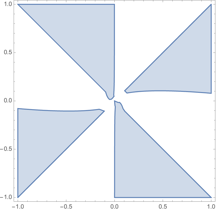
It turns out that wormhole saddle $\sigma_{wh}=\pm\frac{1}{2}\text{i}e^{\frac{\text{i}\pi}{4}}$ is not in this region. For example at $J=1/2$ , $\text{Re}(\langle\Phi^{2}(\sigma_{wh})\rangle_{\text{non-trivial}}-\langle\Phi^{2}(\sigma_{wh})\rangle_{\text{trivial}})=-0.23$ . It suggests that like the 0-dimensional model, the wormhole saddle of $\langle|z|^{2}\rangle$ are within the self-averaging region of the $\sigma$ plane.

8.5 Half-wormholes

With all the results in the previous sections, we expect that the integral (410) can be approximated by

$\displaystyle\|z\|^{2}$	$\displaystyle\approx$	$\displaystyle\int_{\mathbb{R}-0}\frac{\text{d}\sigma}{2\pi}\Psi(\sigma)\Phi(\sigma)+\left(\text{ half-wormholes at }\sigma=0\right),$	(458)
	$\displaystyle=$	$\displaystyle\int_{\mathbb{R}-0}\frac{\text{d}\sigma}{2\pi}\Psi(\sigma)\langle\Phi(\sigma)\rangle+\left(\text{ half-wormholes at }\sigma=0\right),$	(459)
	$\displaystyle=$	$\displaystyle\langle\|z\|^{2}\rangle+\Phi(0)\,,$	(460)

at late time. First we notice that in the late time

\displaystyle\langle\Phi(0)\rangle=2^{N}e^{-\frac{4JTN}{q2^{q}}}\rightarrow 0

(461)

therefore at least (460) is consistent. To confirm (460) we need to compute $\langle\Phi(0)^{2}\rangle$ , $\langle\Phi(0)|z|\rangle$ and the error:

\displaystyle\text{Error}=\langle(|z|^{2}-\langle|z|^{2}\rangle-\Phi(0))^{2}\rangle=\langle|z|^{4}\rangle-\langle|z|^{2}\rangle^{2}+\langle\Phi(0)^{2}\rangle-2\langle|z|^{2}\Phi(0)\rangle.

(462)

In the late time, each term in (462) is given by the non-trivial saddle points. It is clear that $\langle\Phi(0)^{2}\rangle$ , $\langle\Phi(0)|z|\rangle$ can be obtain from $\langle|z|^{4}\rangle$ by setting $g_{12}=0$ . Therefore we have

\displaystyle\text{Error}=\begin{cases}(3-1+2-4)\langle z^{2}\rangle^{2}_{WH}=0&q=4k+2,\\ (2-1+1-2)\langle z^{2}\rangle^{2}_{WH}=0&q=4k,\end{cases}

(463)

therefore (460) indeed is good in the large $T$ limit.

9 Modified Brownian SYK model

In this section, we study the wormhole and half-wormholes contributions in some modified (Brownian) SYK model.

9.1 Brownian SYK with non-vanishing mean value

Let us first consider to turn on the mean value of the random couplings:

\displaystyle\langle J_{A}\rangle=J_{A}^{(0)}=\mu,\quad\langle J_{A}(t)J_{B}(t^{\prime})\rangle=\delta(t-t^{\prime})(\delta_{AB}\tau^{2}+\mu^{2})\,,

(464)

and in this section we use the convention $\{\psi_{i},\psi_{j}\}=2h\delta_{i,j}$ .

Taking the disorder averaging of the coupling we obtain the averaged theory

	$\displaystyle\langle z(T)\rangle_{J}$	$\displaystyle=\int d^{N}\psi\,e^{-S_{a}}\,,$		(465)
	$\displaystyle S_{a}$	$\displaystyle=\frac{1}{2}\int_{0}^{T}dt\sum_{i}^{N}\psi_{i}\partial_{t}\psi_{i}-\text{i}^{q/2}\int dt\sum_{A}J_{A}^{(0)}\psi_{A}-\frac{\tau^{2}}{2}\int dt(\sum_{A}\psi_{A}^{2})$		(466)

We can convert the effective Hamiltonian of the averaged theory as a spin system

\displaystyle\langle z\rangle_{J}=\text{Tr}(e^{-T{\cal H}})\,,\quad{\cal H}=-\text{i}^{q/2}\sum_{A}J_{A}^{(0)}\psi_{A}-\frac{t^{2}}{2}\sum_{A}h^{q}=-\text{i}^{q/2}\sum_{A}J_{A}^{(0)}\psi_{A}-\frac{\tau^{2}}{2}{N\choose q}h^{q}\ .

(467)

When $\mu=0$ , the averaged partition function is given by

\displaystyle\langle z\rangle_{J}=e^{T\frac{\tau^{2}}{2}{N\choose q}h^{q}}\equiv 2^{N}e^{TE_{0}},\quad E_{0}=\frac{\tau^{2}}{2}{N\choose q}h^{q}\sim\frac{\tau^{2}}{2}N^{q}h^{q}\,.

(468)

When $\mu\neq 0$ , we have to evaluate the trace

\displaystyle\langle z\rangle_{J}=e^{TE_{0}}\text{Tr}(e^{T\text{i}^{q/2}\mu\sum_{A}\psi_{A}})=e^{TE_{0}}\int\text{d}^{N}\psi_{i}\exp(T\text{i}^{q/2}\sum_{i}\psi_{i})\ .

(469)

However there is no simple expression for $\langle z\rangle$ . We first consider the simplest case with $q=1$

\displaystyle I_{f}=\int\text{d}^{N}\psi_{i}\exp(a\sum_{i}\psi_{i})\ .

(470)

The idea is to transfer the Majorana fermions to Dirac fermions which have a well-defined rules of integrals. Assuming the total number of fermions is even $N=2K$ then we introduce $K$ Dirac fermions as

	$\displaystyle c_{i}=\frac{1}{2\sqrt{h}}(\psi_{2i-1}-\text{i}\psi_{2i}),\quad c_{i}^{\dagger}=\frac{1}{2\sqrt{h}}(\psi_{2i-1}+\text{i}\psi_{2i}),\quad i=1,\dots,K\,,$		(471)
	$\displaystyle\psi_{2i-1}=\sqrt{h}(c_{i}+c_{i}^{\dagger}),\quad\psi_{2i}=\text{i}\sqrt{h}(c_{i}-c_{i}^{\dagger})\,,$		(472)

which obey

\displaystyle\{c_{i},c_{j}\}

\displaystyle=

\displaystyle\{c_{i}^{\dagger},c_{j}^{\dagger}\}=0,\quad\{c_{i},c_{j}^{\dagger}\}=\delta_{ij}\,

(473)

The integration measure changes as

\displaystyle{\cal D}\psi_{2i}{\cal D}\psi_{2i-1}=2h{\cal D}c_{i}{\cal D}c_{i}^{\dagger}\,.

(475)

Thus the integral can be evaluated as

	$\displaystyle I_{1}$	$\displaystyle=$	$\displaystyle(2h)^{K}\int\prod_{i}{\cal D}c_{i}{\cal D}c_{i}^{\dagger}\exp\left(a\sum_{i}^{K}\sqrt{h}[(1+\text{i})c_{i}+(1-\text{i})c_{i}^{\dagger}]\right)$		(476)
		$\displaystyle=$	$\displaystyle(2h)^{K}(2\cosh(\sqrt{2}ah))^{K}=(2h)^{N}[\cosh(\sqrt{2}ah)]^{N/2}\,.$		(477)

Now we let us consider the case of $q=2$

\displaystyle I_{2}(a)=\int\text{d}^{N}\psi_{i}\exp(\frac{a}{2}\sum_{i\neq j}\psi_{i}A_{ij}\psi_{j}),\quad\text{with }\quad\left(A_{ij}=-A_{ij}=a,\quad i<j\right),

(478)

which looks like a Gaussian but we need to replace $\psi_{i}$ with $c_{i}$ :

	$\displaystyle I_{2}=(\sqrt{2h})^{N}\int\prod_{i}{\cal D}c_{i}{\cal D}c_{i}^{\dagger}\,e^{{\cal H}}$		(479)

	$\displaystyle\quad{\cal H}=\left(\text{i}ah(\sum_{i}^{K}[c_{i}^{\dagger}c_{i}-c_{i}c_{i}^{\dagger}]+2\sum_{i<j}[c_{i}c_{j}-c_{i}^{\dagger}c_{j}^{\dagger}])+2ah\sum_{i<j}[c_{i}^{\dagger}c_{j}+c_{i}c_{j}^{\dagger}]\right)$		(480)

To get an idea how to compute this integral let us consider a simple case of $N=4$ :

	$\displaystyle\psi_{1}=\sqrt{h}(c_{1}+c_{1}^{\dagger}),\psi_{2}=\text{i}\sqrt{h}(c_{1}-c_{1}^{\dagger}),\psi_{3}=\sqrt{h}(c_{2}+c_{2}^{\dagger}),\psi_{4}=\text{i}\sqrt{h}(c_{2}-c_{2}^{\dagger}),$		(481)
	$\displaystyle\sum_{i<j}\psi_{i}\psi_{j}=\text{i}h(c_{1}^{\dagger}c_{1}-c_{1}c_{1}^{\dagger}+c_{2}^{\dagger}c_{2}-c_{2}c_{2}^{\dagger}+2c_{1}c_{2}-2c_{1}^{\dagger}c_{2}^{\dagger})+2h(c_{1}^{\dagger}c_{2}+c_{1}c_{2}^{\dagger}).$		(482)

We have four different states $|\Psi_{i}\rangle$ :

\displaystyle|00\rangle,\quad c_{1}^{\dagger}|00\rangle,\quad c_{2}^{\dagger}|00\rangle,\quad c_{1}^{\dagger}c_{2}^{\dagger}|00\rangle.

(483)

So the operator $\sum_{i<j}\psi_{i}\psi_{j}$ can be written as a $4\times 4$ matrix :

\displaystyle\sum_{i<j}\psi_{i}\psi_{j}=\left(\begin{array}[]{cccc}-2\text{i}h&0&0&-2\text{i}h\\ 0&0&-2h&0\\ 0&2h&0&0\\ -2\text{i}h&0&0&2\text{i}h\\ \end{array}\right)

(488)

with 4 eigenvalues $\{\pm\text{i}2h,\pm\text{i}2\sqrt{2}h\}$ so path integral over $c_{i}$ and $c_{i}^{\dagger}$ can be computed as

\displaystyle\sum_{i}\langle\Psi_{i}|e^{a\sum_{i}\psi_{i}\psi_{j}}|\Psi_{i}\rangle=2\left(\cos(2ah)+\cos(2\sqrt{2}ah)\right)\,.

(489)

For example of $N=6$ , the corresponding matrix is

\displaystyle\sum_{i<j}\psi_{i}\psi_{j}=\left(\begin{array}[]{cccccccc}-3\text{i}h&0&0&0&-2\text{i}h&-2\text{i}h&-2\text{i}h&0\\ 0&-\text{i}h&2h&2h&0&0&0&-2\text{i}h\\ 0&-2h&-\text{i}h&2h&0&0&0&2\text{i}h\\ 0&-2h&-2h&-\text{i}h&0&0&0&-2\text{i}h\\ -2\text{i}h&0&0&0&\text{i}h&2h&-2h&0\\ -2\text{i}h&0&0&0&-2h&\text{i}h&2h&0\\ -2\text{i}h&0&0&0&2h&-2h&\text{i}h&0\\ 0&-2\text{i}h&2\text{i}h&-2\text{i}h&0&0&0&3\text{i}h\\ \end{array}\right)

(498)

which can be divided into two blocks. We get the eigenvalues by directly diagonalizing the matrix:

\displaystyle\pm 5\text{i}h,\quad\pm(2\sqrt{3}+1)\text{i}h,\quad\pm 3\text{i}h,\quad\pm(2\sqrt{3}-1)\text{i}h.

(499)

Similarly for general $N$ , we can write effective Hamiltonian defined in (479) as

\displaystyle{\cal H}=\sum_{i\leq j=1}^{k}\left(\alpha_{ij}c_{i}^{\dagger}c_{j}+\beta_{ij}c_{i}c_{j}^{\dagger}+\gamma_{ij}c_{i}^{\dagger}c_{j}^{\dagger}+\theta_{ij}c_{i}c_{j}\right),

(500)

with

	$\displaystyle\alpha_{ii}=\text{i}h,\quad\beta_{ii}=-\text{i}h,\quad\alpha_{ij}=2h,\quad\beta_{ij}=2h,$		(501)
	$\displaystyle\gamma_{ij}=-2\text{i}h,\quad\theta_{ij}=2\text{i}h,\quad\gamma_{ii}=0,\quad\theta_{ii}=0.$		(502)

This Hamiltonian is quadratic and famously can be diagonalized by the Bogoliubov and Valatin’s method Bogolyubov:1947zz ; Valatin:1958ja . Explicitly we can do the transformation by taking an operator basis for the Hamiltonian

\displaystyle H=c^{\dagger}Mc

(503)

where we have

\displaystyle c^{\dagger}=\left(c_{1}^{\dagger},c_{2}^{\dagger},\dots,c_{1},c_{2},\dots\right).

(504)

In the simple case with $N=4$ the matrix can be expressed as

\displaystyle M=\left(\begin{array}[]{cccc}\text{i}h&h&0&-\text{i}h\\ -h&\text{i}h&\text{i}h&0\\ 0&\text{i}h&-\text{i}h&h\\ -\text{i}h&0&-h&-\text{i}h\\ \end{array}\right),

(509)

we can directly take the diagonalization and get the eigenvalues

\displaystyle\text{i}(1+\sqrt{2})h,\quad-\text{i}(1+\sqrt{2})h,\quad-\text{i}(1-\sqrt{2})h,\quad-\text{i}(-1+\sqrt{2})h.

(510)

For simplicity we take the notation as

\displaystyle\lambda_{1}=\text{i}(\sqrt{2}+1)h,\quad\lambda_{2}=\text{i}(\sqrt{2}-1)h,

(511)

then the resulting effective Hamiltonian becomes

\displaystyle H=\lambda_{1}\left(d_{1}^{\dagger}d_{1}-d_{1}d_{1}^{\dagger}\right)+\lambda_{2}\left(d_{2}^{\dagger}d_{2}-d_{2}d_{2}^{\dagger}\right).

(512)

To evaluate the trace we still take the states as (483) therefore we have

\displaystyle\text{Tr}(e^{H})=e^{-a(\lambda_{1}+\lambda_{2})}+e^{a(\lambda_{1}-\lambda_{2})}+e^{a(-\lambda_{1}+\lambda_{2})}+e^{a(\lambda_{1}+\lambda_{2})},

(513)

so we can recover the result (489). For general $N$ the operator (500) can be expressed as a block matrix

\displaystyle M=\left(\begin{array}[]{cc}A+\text{i}hI_{N}&-\text{i}A\\ \text{i}A&A-\text{i}hI_{N}\end{array}\right),

(516)

with

\displaystyle A=\left(\begin{array}[]{cccc}0&h&h&\cdots\\ -h&0&h&\cdots\\ -h&-h&0&\cdots\\ \vdots&\vdots&\vdots&\ddots\end{array}\right)

(521)

The characteristic equation is

	$\displaystyle\det\left(A+(\text{i}h-\lambda))(A-(\text{i}h+\lambda)-H^{2}\right)$	$\displaystyle=$	$\displaystyle\det\left((h^{2}+\lambda^{2})I_{N}-2\lambda A\right)$		(522)
		$\displaystyle=$	$\displaystyle(\lambda+h)^{N}+(\lambda-h)^{N}=0\,.$		(523)

So the eigenvalues are

\displaystyle\lambda_{m}=\text{i}h\tan(\frac{m\pi}{2N}),\quad m=1,3,\dots,N-1\,.

(524)

then the Hamiltonian becomes

\displaystyle H=\sum_{i=1}^{N}\lambda_{i}(d_{i}^{\dagger}d_{i}-d_{i}d_{i}^{\dagger}).

(525)

and the trace will have the form

\displaystyle{\rm Tr}(e^{H})=\sum_{\sigma=\pm 1}e^{a\sum_{i=1}^{k}\sigma_{i}\lambda_{i}}=\sum_{\sigma}\prod_{i=1}^{k}e^{a\sigma_{i}\lambda_{i}}=\prod_{i=1}^{k}\sum_{\sigma}e^{a\sigma_{i}\lambda_{i}}=2^{k}\prod_{i=1}^{k}\cosh\left(a\lambda_{i}\right)\,,

(526)

Now let us consider the function

\displaystyle X_{n}=\sum_{1\leq i_{1}<\dots i_{n}\leq N}\psi_{i_{1}}\dots\psi_{i_{N}}.

(527)

We would like to argue that in the large $N$ limit, we have the approximation

\displaystyle n!X_{2n}\approx(X_{2})^{n},

(528)

as we find for the 0-dimensional theory. Note that unlike the situation of the 0-dimensional theory, $\{X_{n}\}$ do not form a basis for $X_{2}^{n}$ . For example, let us take $N=6$ , there is indeed the identity

\displaystyle X_{2}^{2}=-15+2!X_{4}

(529)

but we find that

	$\displaystyle X_{2}^{3}$	$\displaystyle=$	$\displaystyle 3!X_{6}+15X_{2}+12(\psi_{1}\psi_{2}+\psi_{1}\psi_{6}+\psi_{3}\psi_{4}+\psi_{4}\psi_{5}+\psi_{5}\psi_{6})$		(530)
			$\displaystyle\qquad-4(\psi_{1}\psi_{4}+\psi_{2}\psi_{4}+\psi_{3}\psi_{6}).$		(530)

Let us focus on the second last term in $X_{2}^{n}$

\displaystyle X_{2}^{n}\approx\dots c_{1}X_{2n-4}+n!X_{2n},\quad c_{1}=(n-2)!{n\choose 2}{N\choose 2}\,,

(531)

where $c_{1}$ is computed as follows. We need to pick 2 $X_{2}$ out of $n$ and contract them, and the $(n-2)$ $X_{2}$ ’s remain not contracted and gives $(n-1)!$ $X_{2n-4}$ . Notice that the subleading term is $X_{2n-4}$ instead of $X_{2n-2}$ , since if we contract one fermion in $X_{2}$ to get

\displaystyle\psi_{1}\psi_{2}\psi_{1}\psi_{3}\mapsto\psi_{3}\psi_{2}\,,

(532)

there is going to be another contraction that gives

\displaystyle\psi_{1}\psi_{3}\psi_{1}\psi_{2}\mapsto\psi_{2}\psi_{3}\ .

(533)

The two outcomes simply cancel with each other. The main conclusion of this computation is, given that $X_{2n}\sim N^{2n}$ , the subleading terms can be safely neglected and approximate $X_{2n}$ by $X_{2}^{n}$ . So in the large $N$ limit, we can use the $G,\Sigma$ trick to compute the fermionic integral

$\displaystyle I_{q}(a)$	$\displaystyle=$	$\displaystyle\int\text{d}^{N}\psi_{i}\exp(a\sum_{A}\psi_{A}),\quad A=\{1\leq a_{1}<\dots<a_{q}\leq N\},$	(534)
	$\displaystyle\approx$	$\displaystyle\int\text{d}^{N}\psi_{i}\,e^{a\frac{G^{\frac{q}{2}}}{\frac{q}{2}!}}e^{\text{i}\sigma(G-\sum_{i<j}\psi_{i}\psi_{j})}\text{d}G\text{d}\sigma$	(535)
	$\displaystyle=$	$\displaystyle\int\text{d}G\text{d}\sigma I_{2}(-\text{i}\sigma)e^{a\frac{G^{\frac{q}{2}}}{\frac{q}{2}!}}e^{\text{i}\sigma G}=I_{2}(\text{i}\partial_{G})e^{a\frac{G^{\frac{q}{2}}}{\frac{q}{2}!}}\|_{G=0}\,.$	(536)

where the function $I_{2}$ is defined in (478). We can evaluate this expression and we expect the half-wormhole contributions to be similar as the $0$ -SYK model

\displaystyle z\approx\langle z\rangle+\Theta\,,\qquad\Theta=\int d^{N}\psi\,e^{-\int_{0}^{T}dt\,\frac{1}{2}\sum_{i}^{N}\psi_{i}\partial_{t}\psi_{i}+\text{i}^{q/2}\int_{0}^{T}dt\sum_{A}(J_{A}-\mu)\psi_{A}}\ .

(537)

The detailed analysis is similar to the Brownian SYK model as we have shown above, but it is not particularly illuminating, so we omit them here.

In the next section, we instead consider a modified SYK-like model where half-wormhole saddle can be verified explicitly.

9.2 Random coupling from product of Grassmann variables $J_{A}^{(0)}=J\prod_{i}\theta_{A_{i}}$

A modified SYK-like model dubbed as partially disorder-averaged SYK model is proposed in Goto:2021wfs . In this model, the random coupling $\widetilde{J}_{A}$ consists of two pieces

\displaystyle\widetilde{J}_{A}=J_{A}+J_{A}^{(0)}

(538)

where $J_{A}$ is the standard random coupling of the SYK model while $J_{A}^{(0)}$ is specially chosen as

\displaystyle J_{i_{i}\dots i_{q}}^{(0)}=\text{i}^{q/2}q!\mu\,\theta_{i_{1}}\dots\theta_{i_{q}},\quad\text{with}\quad\{\theta_{i},\theta_{j}\}={2}\delta_{ij}

(539)

so we can think of it as coupling the fermions $\psi_{i}$ in the original model with some background Majorana fermions $\theta_{i}$ (or non-dynamical fermions living in another universe Goto:2021wfs ). Note that $J_{A}^{(0)}$ is not a c-number which is different from our models studied in the previous section.

9.2.1 0d model

Let us first consider the $0$ -dimensional model to see the difference explicitly. In this case the integral (154) can be written as

	$\displaystyle z$	$\displaystyle=$	$\displaystyle\int\text{d}^{N}\psi\exp(\text{i}^{q/2}\sum\widetilde{J}_{i_{1}\dots i_{q}}\psi_{i_{1}\dots i_{q}})\,$		(540)
		$\displaystyle=$	$\displaystyle\int\text{d}^{N}\psi\exp\left(\text{i}^{q/2}\sum_{A}J_{A}\psi_{A}+\mu(\sum_{i}\theta_{i}\psi_{i})^{q}\right).$		(540)

The averaged quantity $\langle z\rangle$

\displaystyle\langle z\rangle=\int\text{d}^{N}\psi\exp\left(\mu(\sum_{i}\theta_{i}\psi_{i})^{q}\right)\,,

(541)

can be computed in two ways. One can integrate out the fermions $\psi_{i}$ directly. The result is

\displaystyle\langle z\rangle=\frac{\mu^{N/q}N!}{(N/q)!}\int\text{d}^{N}\psi(\theta_{1}\psi_{1})\dots(\theta_{N}\psi_{N})=\left[\prod_{i}\theta_{i}\right]\frac{\mu^{N/q}N!}{(N/q)!}\equiv\left[\prod_{i}\theta_{i}\right]\mathfrak{m}_{p}\,.

(542)

Note that $z$ is not a c-number and depends on the background fermions living in other universe. Here we will not think of this as a problem but a feature since the model is not exactly the original SYK model. Alternatively we can compute this average quantity by the $G,\Sigma$ trick:

	$\displaystyle G_{\sigma}=\sum_{i}\theta_{i}\psi_{i}\,,$
	$\displaystyle\langle z\rangle=\int\text{d}^{N}\psi\int\text{d}G_{\sigma}\frac{\text{d}\Sigma_{\sigma}}{2\pi}e^{\text{i}[\Sigma_{\sigma}(G_{\sigma}-\sum_{i}\theta_{i}\psi_{i})]}e^{\mu G_{\sigma}^{q}}$
	$\displaystyle\qquad=\left[\prod_{i}\theta_{i}\right]\int\text{d}G_{\sigma}\frac{\text{d}\Sigma_{\sigma}}{2\pi}\Sigma_{\sigma}^{N}e^{\text{i}\Sigma_{\sigma}G_{\sigma}+\mu G_{\sigma}^{q}}$		(543)
	$\displaystyle\qquad=\left[\prod_{i}\theta_{i}\right](\partial_{G_{\sigma}})^{N}e^{\mu G_{\sigma}^{q}}\|_{G_{\sigma}=0}=\left[\prod_{i}\theta_{i}\right]\frac{\mu^{N/q}N!}{(N/q)!}\,.$		(544)

One can also use the effective action (543) to derive the large $N$ result of (541) as shown in Goto:2021wfs . We will not repeat that analysis here. Instead, we would like to consider the half-wormhole saddle of $z$

\displaystyle z\approx\langle z\rangle+\Theta

(545)

as we did in last section. The subtlety is that as we stressed $z$ is not a c-number so the approximation (545) is in the sense

\displaystyle\langle[z-(\langle z\rangle+\Theta)]^{2}\rangle\approx 0\,,

(546)

which is a c-number due to (539) is small. Let us proceed by computing the averaged quantity $\langle z^{2}\rangle$

$\displaystyle\langle z^{2}\rangle$	$\displaystyle=$	$\displaystyle\int\text{d}^{2N}\psi\,\exp\left({\frac{\tau^{2}}{q!}}(\sum_{i}\psi_{i}^{L}\psi_{i}^{R})^{q}+\mu(\sum_{i}\theta_{i}\psi_{i}^{L})^{q}+\mu(\sum_{i}\theta_{i}\psi_{i}^{R})^{q}\right)$
	$\displaystyle=$	$\displaystyle\int\text{d}^{2N}\psi\sum_{k}\left(\frac{\tau^{2}}{q!}\right)^{k}\sum_{{i_{1}<\dots<i_{kq}}}(\psi^{LR}_{i_{1}}\dots\psi^{LR}_{i_{qk}})\frac{(qk)!}{k!}\left(\frac{(N-kq)!}{(N/q-k)!}\right)^{2}$
		$\displaystyle\mu^{2p-2k}\sum_{j_{1}<\dots<j_{N-qk}\neq\{i\}}(\theta_{j_{1}}\psi_{j_{1}}^{L})\dots(\theta_{j_{N-qk}}\psi^{L}_{j_{N-kq}})(\theta_{j_{1}}\psi_{j_{1}}^{R})\dots(\theta_{j_{N-k}}\psi^{R}_{j_{N-kq}})$
	$\displaystyle=$	$\displaystyle\int\text{d}^{2N}\psi\sum_{k}\left(\frac{\tau^{2}}{q!}\right)^{k}\mu^{2p-2k}\frac{(qk)!}{k!}\left(\frac{(N-kq)!}{(N/q-k)!}\right)^{2}{N\choose kq}\psi^{LR}_{1}\dots\psi_{N}^{LR}$
	$\displaystyle=$	$\displaystyle\sum_{k}\left(\frac{\tau^{2}}{q!}\right)^{k}\mu^{2p-2k}\frac{(qk)!}{k!}\left(\frac{(N-kq)!}{(N/q-k)!}\right)^{2}{N\choose kq}$
	$\displaystyle=$	$\displaystyle\sum_{k}^{p}\tau^{2k}\mu^{2(p-k)}c_{k}\mathfrak{m}_{p-k}^{2}\equiv\sum_{k}\mathfrak{z}_{2}^{(k)}\,,$	(548)

where $c_{k}$ of defined in (231) and $\mathfrak{m}_{p}$ is defined in (542). The result (9.2.1) is in the same form of (230). So the analysis of the half-wormhole saddle will be similar; we insert the a suitable identity to (540)

	$\displaystyle z$	$\displaystyle=$	$\displaystyle\int\text{d}^{N}\psi\exp(\text{i}^{q/2}\sum\widetilde{J}_{i_{1}\dots i_{q}}\psi_{i_{1}\dots i_{q}})\int\text{d}G_{\sigma}\delta(G_{\sigma}-\sum_{i}\theta_{i}\psi_{i})\exp(\frac{\mu}{q!}(G_{\sigma}^{q}-(\sum_{i}\theta_{i}\psi_{i})^{q}))$		(549)
		$\displaystyle=$	$\displaystyle\int\text{d}^{N}\psi\frac{\text{d}\Sigma_{\sigma}\text{d}G_{\sigma}}{2\pi\text{i}}\exp(\text{i}^{q/2}\sum_{A}J_{A}\psi_{A}+\Sigma_{\sigma}\sum_{i}\theta_{i}\psi_{i})\exp(-\Sigma_{\sigma}G_{\sigma}+\frac{\mu}{q!}G_{\sigma}^{q})\,.$		(549)

Following the arguments below (4.1) one can obtain the half-wormhole saddle¹⁶¹⁶16Here the factor $\prod_{i}\theta_{i}$ should be present.

\displaystyle\Theta=\left[\prod_{i}\theta_{i}\right]\int\text{d}^{N}\psi\exp(\text{i}^{q/2}\sum_{A}J_{A}\psi_{A})\,.

(550)

Then it is easy to find that the half-wormhole saddle satisfies

\displaystyle\langle\Theta\rangle=0,\quad\langle\Theta^{2}\rangle=\langle\Theta z\rangle=\mathfrak{z}_{2}^{(p)}\,,

(551)

so the approximation (545) will be sufficient if $\mathfrak{z}_{2}^{(p)}$ is the dominant term in (548) as we have shown in last section. When $\mathfrak{z}_{2}^{(p)}$ is not the dominant term we have to consider the contribution of fluctuation of $\Sigma_{\sigma}$ . To finish our analysis of the half-wormhole saddle for $z$ , let us redo the computation of $\langle z^{2}\rangle$ with the $G,\Sigma$ trick. We need introduce three $G$ variables

\displaystyle G_{LR}=\frac{1}{N}\sum_{i}\psi_{i}^{L}\psi_{i}^{R},\quad G_{L}=\frac{1}{{N}}\sum_{i}\theta_{i}\psi_{i}^{L},\quad G_{R}=\frac{1}{{N}}\sum_{i}\theta_{i}\psi_{i}^{R}

(552)

then $\langle z^{2}\rangle$ can be written as

$\displaystyle\langle z^{2}\rangle$	$\displaystyle=$	$\displaystyle\int\text{d}^{2N}\psi\prod_{a}\text{d}G_{a}\exp\left(\frac{N}{q}(tG_{LR}^{q}+uG_{L}^{q}+uG_{R}^{q})\right)\int\prod_{a}\frac{d\Sigma_{a}}{2\pi\text{i}/N}\exp(-\Sigma_{LR}(NG_{LR}-\sum_{i}\psi_{i}^{L}\psi_{i}^{R}))$	(553)
		$\displaystyle\exp(-\Sigma_{L}(NG_{L}-\sum_{i}\theta_{i}\psi_{i}^{L}))\exp(-\Sigma_{R}(NG_{R}-\sum_{i}\theta_{i}\psi_{i}^{R}))$
	$\displaystyle=$	$\displaystyle\int[\prod_{a}\text{d}G_{a}\frac{d\Sigma_{a}}{2\pi\text{i}/N}]\exp\left(N(\frac{t}{q}G_{LR}^{q}+\frac{u}{q}G_{L}^{q}+\frac{u}{q}G_{R}^{q}-\sum_{a}\Sigma_{a}G_{a})\right)(\Sigma_{LR}+\Sigma_{L}\Sigma_{R})^{N}\,,$

where in order to have a well-defined large $N$ scaling we have introduced

\displaystyle t=\frac{\tau^{2}}{(q-1)!}N^{q-1},\quad u=q\mu N^{q-1}.

(554)

The saddle point equations are

	$\displaystyle tG_{LR}^{q-1}=\Sigma_{LR},\quad uG_{L}^{q-1}=\Sigma_{L},\quad uG_{R}^{q-1}=\Sigma_{R}\,,$		(555)
	$\displaystyle G_{LR}=\frac{1}{\Sigma_{LR}+\Sigma_{L}\Sigma_{R}},\quad G_{L}=-\frac{\Sigma_{R}}{\Sigma_{LR}+\Sigma_{L}\Sigma_{R}},\quad G_{R}=-\frac{\Sigma_{L}}{\Sigma_{LR}+\Sigma_{L}\Sigma_{R}}\,.$		(556)

The obvious solutions are the “wormhole” saddles with

\displaystyle G_{L}=G_{R}=\Sigma_{L}=\Sigma_{R}=0,

(557)

which corresponds to $\mathfrak{z}_{2}^{p}$ . There are also other saddles corresponding to other $\mathfrak{z}_{2}^{k}$ . For the simplest case $q=2$ , these solutions can be written explicitly. The “wormhole” saddles are

	$\displaystyle G_{L}=G_{R}=\Sigma_{L}=\Sigma_{R}=0,G_{LR}=\pm\frac{1}{\sqrt{t}},\quad\Sigma_{LR}=\pm\sqrt{t},$		(558)
	$\displaystyle\langle z^{2}\rangle_{\text{WH}}=e^{-\frac{N}{2}}t^{N/2}\,,$		(559)

which do not depend on $\mu$ and the other four solutions are

	$\displaystyle\Sigma_{L}=\Sigma_{R}=uG_{L}=uG_{R}=\pm\sqrt{\frac{u^{2}-t}{u}},\quad\Sigma_{LR}=\frac{t}{u},\quad G_{LR}=\frac{1}{u}$		(560)
	$\displaystyle\Sigma_{L}=uG_{L}=-\Sigma_{R}=-uG_{R}=\pm\sqrt{\frac{u^{2}-t}{u}},\quad\Sigma_{LR}=-\frac{{t}}{u},\quad G_{LR}=-\frac{1}{u}\,,$		(561)
	$\displaystyle\langle z^{2}\rangle_{\text{new}}=e^{-\frac{N}{2}(2-\frac{t}{u^{2}})}u^{N}$		(562)

Apparently when $u\rightarrow\infty$ , $\Sigma_{LR},G_{LR}\rightarrow 0,$ then we expect that in this limit the dominant saddle will correspond to $\mathfrak{z}_{2}^{0}$ since in this limit saddle point value does not depend on $t$ . Comparing these two saddle values we find

\displaystyle\frac{\langle z^{2}\rangle_{\text{WH}}}{\langle z^{2}\rangle_{\text{new}}}=\exp\left(\frac{N}{2}(1-x+\log x)\right)\leq 1,\quad x=\frac{t}{u^{2}}\,.

(563)

Note that when $x=1$ such that $\langle z^{2}\rangle_{\text{WH}}=\langle z^{2}\rangle_{\text{new}}$ the new saddle just reduces to the wormhole saddle. Therefore it implies that the new saddle always dominates.

This new saddle is named as “unlinked half-wormhole” in Goto:2021wfs to distinguish it from the half-wormhole saddle which was found in Saad:2021rcu . One interpretation of this new saddle is that it is the analogue of the disconnected saddle in this model; indeed, we do not find other disconnected saddle with $G_{LR}=0$ , $\Sigma_{LR}=0$ and $G_{L/R},\Sigma_{L/R}\neq 0$ , in addition, this saddle is present only when $u\neq 0$ , and this saddle is more and more important as $u$ increases.

The analysis of the half-wormhole saddle for $z^{2}$ will be similar to one we did in last section so we will not repeat here.

9.2.2 1d model

Now we come back to the 0+1d model that is a variant of the Brownian SYK model. Let us begin by deriving the wormhole saddle of $\langle z^{2}\rangle$ ¹⁷¹⁷17Here we have assumed the large $N$ limit, the exact treatment can be found in Saad:2021rcu

	$\displaystyle z_{L}z_{R}=\int\text{d}^{2N}\psi\exp\left\{-\int_{0}^{T}\text{d}t\frac{1}{2}\sum_{i}(\psi_{i}^{L}\partial_{t}\psi_{i}^{L}+\psi_{i}^{R}\partial_{t}\psi_{i}^{R})+\text{i}^{q/2}\int_{0}^{T}\text{d}t\sum_{A}\tilde{J}_{A}(\psi_{A}^{L}+\psi_{A}^{R})\right\}$
	$\displaystyle\langle z_{L}z_{R}\rangle=\int\text{d}^{2N}\psi\exp\left\{-\int_{0}^{T}\text{d}t\frac{1}{2}\sum_{i}(\psi_{i}^{L}\partial_{t}\psi_{i}^{L}+\psi_{i}^{R}\partial_{t}\psi_{i}^{R})+\right.$
	$\displaystyle\qquad\qquad\qquad\left.\int_{0}^{T}\text{d}t\left({\frac{\tau^{2}}{q!}}(\sum_{i}\psi_{i}^{L}\psi_{i}^{R})^{q}+\mu(\sum_{i}\theta_{i}\psi_{i}^{L})^{q}+\mu(\sum_{i}\theta_{i}\psi_{i}^{R})^{q}\right)+\tau^{2}E_{0}T\right\}\,.$		(564)
	$\displaystyle\qquad\qquad=\int\text{d}^{2N}\psi[\prod_{a}\text{d}G_{a}\frac{d\Sigma_{a}}{2\pi\text{i}}]\exp\left\{-\int_{0}^{T}\text{d}t\frac{1}{2}\sum_{i}(\psi_{i}^{L}\partial_{t}\psi_{i}^{L}+\psi_{i}^{R}\partial_{t}\psi_{i}^{R})+\tau^{2}TE_{0}+\right.$
	$\displaystyle\qquad\left.\int_{0}^{T}\text{d}t\left(\frac{\tau^{2}}{q!}G_{LR}^{q}+\mu G_{L}^{q}+\mu G_{R}^{q}-\sum_{a}\Sigma_{a}G_{a}+\sum_{i}[\Sigma_{LR}\psi_{i}^{L}\psi_{i}^{R}+\Sigma_{L}\theta_{i}\psi_{i}^{L}+\Sigma_{R}\theta_{i}\psi_{i}^{R}]\right)\right\}\,,$

where $E_{0}={N\choose q}$ is the constant term coming from $\psi_{A}^{L(R)}\psi_{A}^{L(R)}=(-1)^{\frac{q}{2}}$ . As explained in Saad:2021rcu , we can focus on the time-independent saddles then the fermions can be simply integrated out. The result is ¹⁸¹⁸18This is result is different from the one derived in Goto:2021wfs . It seems that they used a wrong formula for the fermion integral.

	$\displaystyle\langle z_{L}z_{R}\rangle$	$\displaystyle=$	$\displaystyle e^{T\tau^{2}E_{0}}\int[\prod_{a}\text{d}G_{a}\frac{d\Sigma_{a}}{2\pi\text{i}}]e^{TN(\frac{t}{q}G_{LR}^{q}+\frac{u}{q}G_{L}^{q}+\frac{u}{q}G_{R}^{q}-\sum_{a}\Sigma_{a}G_{a})}[\cosh(T\sqrt{\Sigma_{L}^{2}+\Sigma_{R}^{2}-\Sigma_{LR}^{2}})]^{N}.$		(566)
		$\displaystyle=$	$\displaystyle\int[\prod_{a}\text{d}G_{a}\frac{d\Sigma_{a}}{2\pi\text{i}}]e^{\tau^{2}TE_{0}}e^{S_{eff}}$		(566)

For general $T$ , the saddle equation is very hard to solve due to the complicity of $\cosh$ function. However the equations simplify in the large $T$ limit because of the following approximations

\displaystyle\log(\cosh(T\sqrt{\Sigma_{L}^{2}+\Sigma_{R}^{2}-\Sigma_{LR}^{2}}))\approx\pm\text{i}T\sqrt{\Sigma_{LR}^{2}-\Sigma_{L}^{2}-\Sigma_{R}^{2}}\,.

(567)

Then in this limit the effective action becomes

\displaystyle S_{eff}=TN(\frac{t}{q}G_{LR}^{q}+\frac{u}{q}G_{L}^{q}+\frac{u}{q}G_{R}^{q}-\sum_{a}\Sigma_{a}G_{a})\pm\text{i}NT\sqrt{\Sigma_{LR}^{2}-\Sigma_{L}^{2}-\Sigma_{R}^{2}}\,,

(568)

and corresponding saddle point equations are

	$\displaystyle tG_{LR}^{q-1}=\Sigma_{LR},\quad uG_{L}^{q-1}=\Sigma_{L},\quad uG_{R}^{q-1}=\Sigma_{R},$		(569)
	$\displaystyle G_{LR}=\pm\frac{\text{i}\Sigma_{LR}}{\sqrt{\Sigma_{LR}^{2}-\Sigma_{L}^{2}-\Sigma_{R}^{2}}}\,,$		(570)
	$\displaystyle G_{L}=\mp\frac{\text{i}\Sigma_{L}}{\sqrt{\Sigma_{LR}^{2}-\Sigma_{L}^{2}-\Sigma_{R}^{2}}},\quad G_{R}=\mp\frac{\text{i}\Sigma_{R}}{\sqrt{\Sigma_{LR}^{2}-\Sigma_{L}^{2}-\Sigma_{R}^{2}}}\,.$		(571)

So the wormhole saddle still presents Saad:2018bqo

	$\displaystyle G_{L}=G_{R}=\Sigma_{L}=\Sigma_{R}=0,\quad G_{LR}=\pm\text{i},$		(572)
	$\displaystyle e^{S_{eff}}\Big{\|}_{\text{WH}}=e^{\text{i}^{q}TN\frac{t}{q}}.$		(573)

The unlinked half-wormhole saddle is:

	$\displaystyle G_{LR}=\Sigma_{LR}=0,\quad G_{L}=\sin\alpha,\quad G_{R}=\cos\alpha,$		(574)
	$\displaystyle e^{S_{eff}}\Big{\|}_{\text{unlink}}=e^{TN\frac{u}{q}(\cos^{q}\alpha+\sin^{q}\alpha)}\leq e^{S_{eff}}\Big{\|}_{\text{unlink},\alpha=0,\pi/2}=e^{TN\frac{u}{q}}\,$		(575)

where the relation

\displaystyle G_{L}^{2}+G_{R}^{2}-G_{LR}^{2}=1\,,

(576)

is fulfilled and $\alpha$ satisfies

\displaystyle\cos\alpha=\pm\frac{\cos^{q-1}\alpha}{\sqrt{\cos^{2q-2}\alpha+\sin^{2q-2}\alpha}}.

(577)

In the late time $(T\rightarrow\infty)$ , there is indeed a wormhole saddle so it possible to include a linked half-wormhole saddle for $z$ . We also assume that the half-wormhole saddle is time independent since the wormhole saddle is time independent. Then the analysis is completely same as the one for the 0-dimensional model. So the half-wormhole saddle will be given by

	$\displaystyle\Theta=\left[\prod_{i}\theta_{i}\right]\int\text{d}^{N}\psi\exp(T\text{i}^{q/2}\sum_{A}J_{A}\psi_{A})\,,$		(578)
	$\displaystyle\langle\Theta^{2}\rangle\approx\langle\Theta z\rangle\approx\langle z_{L}z_{R}\rangle\|_{\text{Wormhole saddle}}\,.$		(579)

10 Discussion

In this paper we consider the half-wormhole proposal in some statistical models and simple SYK-like models. We showed that in all statistical models we have consider the half-wormhole conjecture (63) is valid almost for all the distributions except for some special cases where the mean value of the random variable vanish. In the 0-dimensional SYK model which is introduced in Saad:2021rcu we have shown that the half-wormhole construction depends on the distribution of the couplings. When the mean value of the coupling is very large then only the disconnected saddles dominate therefore the correlation functions automatically factorize. If the mean value is very small such that only the wormhole saddles dominate then factorization can be restored by adding half-wormhole saddles. When the disconnected saddles and wormhole saddles are comparable, we have to modified the half-wormhole saddle to restore the factorization. We also generalized $G,\Sigma$ trick to compute $\langle z\rangle$ . As a by-product, we can construct a a new saddle, the single half-wormhole saddle, for $z$ . Moreover we argued if the random couplings satisfy a general distribution, new half-wormhole saddles can be constructed ¹⁹¹⁹19Interestingly, irrelevant deformation of 0-SYK model is studied in Das:2022uhj where they show after deformation half-wormhole saddle survives. It is very possible that our new half-wormholes will also survive under the same irrelevant deformation.. We also generalize the construction of half-wormhole saddles to (modified) Brownian SYK model.

Partially averaged models and spacetime branes

The meaning of higher cumulants of the random coupling can be understood from the idea of Coleman’s Coleman:1988cy and Giddings’s and Strominger’s Giddings:1988wv ; Giddings:1988cx . Just as we showed they are related to the non-local interaction induced by the spacetime wormholes. However the first cumulant or the mean value seems to be puzzling. In Blommaert:2021gha ; Goto:2021wfs , ensemble theories with non-vanishing mean value random couplings are also consider where they call such models partially averaged models. In these models, the mean values of random couplings can be understood as external sources or spacetime branes which describe the non-perturbative corrections. It is shown in Blommaert:2021fob by fine tuning these non-perturbative corrections the JT gravity can factorize for all orders. But it seems that the original half-wormhole Saad:2021rcu constructed in 0-SYK model is not related to the branes but just a result of applying $G,\Sigma$ trick in the non-averaged theory. However we can understand this construction in an opposite way: the half-wormhole is constructed by adding eigenbranes Blommaert:2019wfy ; Goel:2020yxl in the averaged theory. This opposite point of view can also be viewed as an explicit realization of the idea Saad:2021uzi about factorization.

Standard SYK model

There are already proposals Saad:2021uzi ; Mukhametzhanov:2021hdi ; Mukhametzhanov:2021nea ; Goto:2021wfs of the half-wormhole saddle for $z^{2}$ in the standard SYK model. But due to technical difficulty it has not been confirmed. It would be interesting to generalize our single half-wormhole saddle to the SYK model since $z$ is much simpler than $z^{2}$ . It would be also interesting to generalize the new half-wormholes we found in section 3 to the standard SYK model and understand their possible relations to saddles in JT gravity.

Non-trivial saddles and Null states

In the simple 0-dimensional SYK model and Brownian SYK model, we find some non-trivial saddles whose on-shell values are comparable with one of the trivial self-averaging saddles. It would be very interesting if such non-trivial saddle also exists in the standard SYK model. It implies that there are also some non-trivial solutions in the dual (deformed) JT gravity. In the semiclassical physics, this coexistence of bulk description can be understood as the consequence of null states. In Blommaert:2022ucs , the null states of (deformed) JT gravity are proposed. However these null states do not show up in the dual matrix model. It seems to be promising to identify these null states in the SYK model.

Acknowledgements.

We thank many of the members of KITS for interesting related discussions. We also want to thank Kenta Suzuki for comments on a draft of this paper. CP is supported by the Fundamental Research Funds for the Central Universities, by funds from the University of Chinese Academy of Science (UCAS), and funds from the Kavli Institute for Theoretical Science (KITS). JT is supported by the National Youth Fund No.12105289 and funds from the UCAS program of special research associate.

Appendix A Explicit examples: simple observables

Thanks to the central limit theorem (CLT), the simplest choice of $Y(X)$ is just the summation of $N$ independent and identical random samples. We will first check proposal with three explicit distributions: the Gaussian distribution, the exponential distribution and the Poisson distribution and then give a general proof for general cases. Readers who are bored with these examples can jump into the general proof directly.

Let $Y$ to be a summation of $N$ independent and identical random variables, i.e.

\displaystyle Y=\sum_{i=1}^{N}X_{i},\quad Y^{2}=\sum_{i,j}^{N}X_{i}X_{j}.

(580)

$\bullet$ Gaussian distribution

The PDF of Gaussian distribution $\mathcal{N}(\mu,t^{2})$ is

\displaystyle P(x)=\frac{1}{t\sqrt{2\pi}}e^{-\frac{1}{2}(\frac{x-\mu}{t})^{2}}.

(581)

Given (581) one can straightforwardly compute the averaged quantities

	$\displaystyle\langle X_{i}\rangle=\mu,\quad\langle e^{\text{i}k_{i}X_{i}}\rangle=e^{-\frac{k_{i}^{2}t^{2}}{2}+\text{i}k_{i}\mu},\quad\langle Y^{2}\rangle=Nt^{2}+N^{2}\mu^{2},$		(582)
	$\displaystyle\frac{\langle Ye^{\sum_{i}\text{i}k_{i}X_{i}}\rangle}{\langle e^{\text{i}\sum_{i}k_{i}X_{i}}\rangle}=\sum_{i}\frac{\langle x_{i}e^{\text{i}k_{i}x_{i}}\rangle}{\langle e^{\text{i}k_{i}x_{i}}\rangle}\equiv\sum_{i}k_{i}[1],\quad k_{i}[1]=(u+\text{i}k_{i}t^{2}).$		(583)

where we have defined

\displaystyle k_{i}[n]=\frac{\langle x^{n}_{i}e^{\text{i}k_{i}x_{i}}\rangle}{\langle e^{\text{i}k_{i}x_{i}}\rangle}.

(584)

Let us introduce another convenient quantity

	$\displaystyle\widehat{k_{i}[n]^{m}}=\frac{1}{2\pi}\int dk_{i}\frac{e^{-\text{i}k_{i}X_{i}}}{P(X_{i})}\langle e^{\text{i}k_{i}x_{i}}\rangle k_{i}[n]^{m},$		(585)
	$\displaystyle\widehat{k_{i}[1]}=X_{i},\quad\widehat{k_{i}[1]^{2}}=X_{i}^{2}-t^{2},\quad\dots$		(586)

then the half-wormhole can be written as

	$\displaystyle\Phi$	$\displaystyle=$	$\displaystyle\sum_{i}\widehat{k_{i}[1]^{2}}+\sum_{i\neq j}\widehat{k_{i}[1]}\widehat{k_{j}[1]}=\sum_{i}(X_{i}^{2}-t^{2})+\sum_{i\neq j}X_{i}X_{j},$		(587)
		$\displaystyle=$	$\displaystyle Y^{2}-Nt^{2}$		(588)

Substituting into (20) one can computed the error and the ration $\rho$ directly

	Error	$\displaystyle=$	$\displaystyle Y^{2}-\left(Nt^{2}+N^{2}\mu^{2}-N^{2}\mu^{2}+Y^{2}-Nt^{2}\right)$		(589)
		$\displaystyle=$	$\displaystyle 0.$		(590)

The proposal is exact as expected.

$\bullet$ Exponential distribution

The PDF of exponential distribution is given by

\displaystyle P_{\lambda}(x)=\begin{cases}\lambda e^{-\lambda x},\quad&x\geq 0,\\ 0,&x<0,\end{cases}

(591)

and the moments are given by

\displaystyle\langle x^{n}\rangle=\frac{n!}{\lambda^{n}}.

(592)

The relevant averaged quantities are

\displaystyle\langle X_{i}\rangle=\frac{1}{\lambda},\quad\langle e^{\text{i}kX_{i}}\rangle=\frac{\lambda}{\lambda-\text{i}k},\quad\langle Y^{2}\rangle=\frac{N(N+1)}{\lambda^{2}}.

(593)

From the example of Gaussian distribution we have shown that to compute $\Phi$ (588) and the error (589) we only need to compute

\displaystyle\widehat{k_{i}[1]}=X_{i},\quad\widehat{k_{i}[1]^{2}}=\frac{X_{i}^{2}}{2},

(594)

which lead to

\displaystyle\text{Error}=\sum_{i}\left(\frac{X_{i}^{2}}{2}-\frac{1}{\lambda^{2}}\right),\quad\rho\approx\frac{\langle\text{Error}^{2}\rangle}{\langle Y^{2}\rangle^{2}}\sim\frac{1}{N^{3}}.

(595)

So the proposal is correct.

$\bullet$ Poisson distribution

Next let us examine the proposal for a discrete probability distribution: the Poisson distribution. The PDF is

\displaystyle P_{\lambda}(k)=\frac{e^{-\lambda}\lambda^{k}}{k!},\quad k=0,1,2,\dots

(596)

and the moments are given by

\displaystyle\langle x^{n}\rangle=B_{n}(\lambda),

(597)

where $B_{n}(\lambda)$ is the Bell polynomial. The relevant averaged quantities can be easily computed

	$\displaystyle\langle X_{i}\rangle={\lambda},\quad\langle e^{\text{i}kX_{i}}\rangle=e^{-\lambda+e^{\text{i}k}\lambda},\quad\langle Y^{2}\rangle=N\lambda+N^{2}\lambda^{2},$		(598)
	$\displaystyle k_{i}[1]=e^{\text{i}k_{i}}\lambda.$		(599)

The computation of $\widehat{k_{i}[1]}$ and $\widehat{k_{i}[1]^{2}}$ is a little subtle and needs some explanation. According to the definition (585), we have

	$\displaystyle\widehat{k_{i}[1]}$	$\displaystyle=$	$\displaystyle\frac{\lambda}{2\pi P(X_{i})}\int dk_{i}{e^{-\text{i}k_{i}X_{i}}}{}\langle e^{\text{i}k_{i}x_{i}}\rangle e^{\text{i}k_{i}},$		(600)
		$\displaystyle=$	$\displaystyle\frac{\lambda}{P(X_{i})}P(X_{i}-1)=X_{i},$		(601)

where in the second line we have used the fact that the inverse Fourier transformation of the characteristic function is the PDF

\displaystyle\frac{1}{2\pi}\int dk_{i}{e^{-\text{i}k_{i}X_{i}}}{}\langle e^{\text{i}k_{i}x_{i}}\rangle=P(X_{i}).

(602)

Similarly one can derive

\displaystyle\widehat{k_{i}[1]^{2}}

\displaystyle=

\displaystyle\lambda^{2}\frac{P(X_{i}-2)}{P(X_{i})}=X_{i}(X_{i}-1).

(603)

Then using (589) we can obtain the error

\displaystyle\text{Error}=\sum_{i}(X_{i}-\lambda),\quad\rho\approx\frac{\langle\text{Error}^{2}\rangle}{\langle Y^{2}\rangle^{2}}\sim\frac{1}{N^{3}},

(604)

so the proposal is correct while the effective parameter is $\lambda N$ instead of $N$ .

Appendix B Explicite Examples: composite observables

Gaussian distribution

We still start from the simple model

\displaystyle Y=\sum_{i=1}^{N}X_{i}^{2},\quad\langle X_{i}^{2}\rangle=t^{2},\quad Y^{2}=\sum_{i,j}X_{i}^{2}X_{j}^{2}.

(605)

It is easy to evaluate

	$\displaystyle\langle e^{\text{i}k_{i}X_{i}}\rangle=\exp(-\sum_{i}\frac{k_{i}^{2}t^{2}}{2}),$		(606)
	$\displaystyle\langle Ye^{\text{i}\sum_{i}k_{i}X_{i}}\rangle/\langle e^{\text{i}\sum_{i}k_{i}X_{i}}\rangle=\sum_{i}(-k_{i}^{2}t^{4}+t^{2}).$		(607)

Then we find

\displaystyle\Phi=\sum_{i}\left(X_{i}^{4}-4t^{2}X_{i}^{2}+2t^{4}\right)+\sum_{i\neq j}X_{i}^{2}X_{j}^{2},

(608)

and the error is given by

\displaystyle\text{Error}=4Nt^{4}-4t^{2}\sum_{i}X_{i}^{2}.

(609)

From this we can easily find that the proposal is correct.

Let us consider

	$\displaystyle Y=\sum_{i}X_{i}^{3},\quad\langle X_{i}^{3}\rangle=0,$		(610)
	$\displaystyle Y^{2}=\sum_{i,j}X_{i}^{3}X_{j}^{3},\quad\langle Y^{2}\rangle=15Nt^{6}.$		(611)

Then we find can evaluate

\displaystyle\langle Ye^{\text{i}k_{i}X_{i}}\rangle/\langle e^{\text{i}k_{i}X_{i}}\rangle=\sum_{i}\text{i}k_{i}t^{4}(3-k_{i}^{2}t^{2}),

(612)

and

\displaystyle\Phi=\sum_{i}(X_{i}^{6}-9t^{2}X_{i}^{4}+18t^{4}X_{i}^{2}-6t^{6})+\sum_{i\neq j}X_{i}^{3}X_{j}^{3}.

(613)

So that the error is given by

\displaystyle\text{Error}=\sum_{i}(9t^{2}X_{i}^{4}-18t^{4}X_{i}^{2}-9t^{6}),

(614)

the leading order of $\langle\text{Error}^{2}\rangle$ is

\displaystyle 0N^{2}.

(615)

Let us consider

\displaystyle Y=\sum_{i}X_{i}^{4},\quad\langle X_{i}^{4}\rangle=3t^{4},\quad Y^{2}=\sum_{i,j}X_{i}^{4}X_{j}^{4}

(616)

then we find can evaluate

\displaystyle\langle Ye^{\text{i}k_{i}X_{i}}\rangle/\langle e^{\text{i}k_{i}X_{i}}\rangle=\sum_{i}t^{4}(k_{i}^{4}t^{4}-6k_{i}^{2}t^{2}+3)

(617)

and

\displaystyle\Phi=8\sum_{i}(3t^{8}-12t^{6}X_{i}^{2}+9t^{3}X_{i}^{4}-2t^{2}X_{i}^{6})+Y^{2}

(618)

such that the error is

\displaystyle\text{Error}=-8\sum_{i}(15t^{8}-12t^{6}X_{i}^{2}+9t^{3}X_{i}^{4}-2t^{2}X_{i}^{6}).

(619)

We can also find the leading order of $\langle\text{Error}^{2}\rangle$ is zero.

In general let us consider

\displaystyle Y=\sum_{i}e^{mX_{i}},\quad\langle e^{mX_{i}}\rangle=e^{\frac{m^{2}t^{2}}{2}},\quad Y^{2}=\sum_{i,j}e^{mX_{i}}e^{mX_{j}},

(620)

and

\displaystyle\Phi=\sum_{i}(e^{m(-mt^{2}+2X_{i})}-e^{2mX_{i}})+Y^{2},

(621)

such that

\displaystyle\text{Error}=\sum_{i}(e^{-m^{2}t^{2}}-1)(e^{2m^{2}t^{2}}-e^{2mX_{i}}),

(622)

\displaystyle\langle\text{Error}^{2}\rangle=Ne^{4m^{2}t^{2}}(e^{4m^{2}t^{2}}-1)(e^{-m^{2}t^{2}}-1)^{2},

(623)

which is sub-dominant comparing to $\langle Y^{2}\rangle^{2}$ .

Exponential distribution

First let us choose

\displaystyle Y=\sum_{i}X_{i}^{2},\quad\langle X_{i}^{2}\rangle=\frac{2}{\lambda^{2}},\quad Y^{2}=\sum_{i,j}X_{i}^{2}X_{j}^{2}.

(624)

Correspondingly we find

\displaystyle\frac{\langle Ye^{\text{i}kX_{i}}\rangle}{\langle e^{\text{i}kX_{i}}\rangle}=-\frac{2}{(k+\text{i}\lambda)^{2}}

(625)

and

\displaystyle\Phi

\displaystyle=

\displaystyle-\frac{5}{6}\sum_{i}X_{i}^{4}+\sum_{i,j}X_{i}^{2}X_{j}^{2}.

(626)

So the error is given by

	$\displaystyle\text{Error}=\sum_{i}\left(\frac{5X_{i}^{4}}{6}-\frac{20}{\lambda^{4}}\right),$		(627)
	$\displaystyle\langle\text{Error}^{2}\rangle=\frac{25N}{36\lambda^{8}}(8!-4!^{2}).$		(628)

In general, let us consider

\displaystyle Y=\sum_{i}e^{\beta X_{i}},\quad\langle e^{\beta X_{i}}\rangle=\frac{\lambda}{\lambda-\beta},\quad Y^{2}=\sum_{i,j}e^{\beta X_{i}}e^{\beta X_{j}}.

(629)

Then we can obtain

\displaystyle\Phi

\displaystyle=

\displaystyle\sum_{i}\left(e^{\beta X_{i}}(1-e^{\beta X_{i}}+\beta X_{i})\right)+\sum_{i,j}e^{\beta X_{i}}e^{\beta X_{j}}.

(630)

So the error is

	$\displaystyle\text{Error}=\sum_{i}\left(e^{2\beta X_{i}}-e^{\beta X_{i}}(1+\beta X_{i})\right)-\frac{N\beta^{2}\lambda}{(\beta-\lambda)^{2}(\lambda-2\beta)},$		(631)
	$\displaystyle\langle\text{Error}^{2}\rangle=N\left(\frac{2\beta^{4}(3\lambda-8\beta)}{(2\beta-\lambda)^{3}(4\beta-\lambda)(\lambda-3\beta)}-\frac{\lambda^{2}\beta^{4}}{(\lambda-\beta)^{4}(\lambda-2\beta)^{2}}\right),$		(632)

given that the condition

\displaystyle\beta<\frac{\lambda}{4},

(633)

to ensure that all the integrals to be convergent.

Poisson distribution

Let us choose

\displaystyle Y=\sum_{i}X_{i}^{2},\quad\langle X_{i}^{2}\rangle=\lambda^{2}+\lambda,\quad Y^{2}=\sum_{i,j}X_{i}^{2}X_{j}^{2}

(634)

Then we find

\displaystyle\frac{\langle Ye^{\text{i}k_{i}X_{i}}\rangle}{\langle e^{\text{i}k_{i}X_{i}}\rangle}=\sum_{i}\lambda e^{\text{i}k_{i}}(1+\lambda e^{\text{i}k_{i}})

(635)

and

\displaystyle\Phi=\sum_{i}\left(X_{i}(-3+6X_{i}-4X_{i}^{2})\right)+\sum_{i,j}X_{i}^{2}X_{j}^{2}.

(636)

Therefore the error is

	$\displaystyle\text{Error}=\sum_{i}\left(X_{i}(3-6X_{i}+4X_{i}^{2})-\lambda(1+6\lambda+4\lambda^{2})\right)$		(637)
	$\displaystyle\langle\text{Error}^{2}\rangle=N\lambda(24\lambda(\lambda(6\lambda(\lambda+4)+23)+4)+1)$		(638)
	$\displaystyle\frac{\langle\text{Error}^{2}\rangle}{\langle Y^{2}\rangle^{2}}\sim\frac{1}{N^{3}}$		(639)

In general let us consider

\displaystyle Y=\sum_{i}e^{\beta X_{i}},\quad\langle e^{\beta X_{i}}\rangle=\exp\lambda(e^{\beta}-1),\quad Y^{2}=\sum_{i,j}e^{\beta X_{i}}e^{\beta X_{j}}.

(640)

Then we find

\displaystyle\frac{\langle Ye^{\text{i}k_{i}X_{i}}\rangle}{\langle e^{\text{i}k_{i}X_{i}}\rangle}=e^{\left(e^{\beta}-1\right)e^{\text{i}k_{i}}\lambda}

(641)

and

\displaystyle\Phi

\displaystyle=

\displaystyle\sum_{i}(\left(2e^{\beta}-1\right)^{X_{i}}-e^{2\beta X_{i}})+Y^{2}.

(642)

Therefore the error is

	$\displaystyle\text{Error}=\sum_{i}\left(-\left(2e^{\beta}-1\right)^{X_{i}}+e^{2\beta X_{i}}-e^{-2\lambda}\left(e^{e^{2\beta}\lambda+\lambda}-e^{2e^{\beta}\lambda}\right)\right)$		(643)
	$\displaystyle\langle\text{Error}^{2}\rangle=-e^{-4\lambda}N\left(e^{4e^{\beta}\lambda}-2e^{\left(e^{\beta}+1\right)^{2}\lambda}+e^{2\left(e^{2\beta}+1\right)\lambda}-e^{\left(e^{4\beta}+3\right)\lambda}-e^{4\left(e^{\beta}\left(e^{\beta}-1\right)+1\right)\lambda}+2e^{\left(e^{2\beta}\left(2e^{\beta}-1\right)+3\right)\lambda}\right)$

and

\displaystyle\frac{\langle\text{Error}^{2}\rangle}{\langle Y^{2}\rangle^{2}}\sim\frac{1}{N^{3}}.

(645)

Appendix C Explicte Examples: generalized statistical models

The exponential distribution

First let us consider the exponential distribution. It is straightforward to derive

	$\displaystyle\langle Y\rangle=\langle\sum_{i\neq j}X_{i}X_{j}\rangle=N(N-1)\frac{1}{\lambda^{2}},$		(646)
	$\displaystyle\langle Y^{2}\rangle=\frac{2N(N-1)(2N-1)+N^{2}(N-1)^{2}}{\lambda^{4}}$		(647)

and

\displaystyle\Phi

\displaystyle=

\displaystyle\sum_{i\neq j\neq p\neq q}X_{i}X_{j}X_{p}X_{q}+4\sum_{i\neq j\neq p}\frac{X_{i}^{2}}{2}X_{j}X_{p}+2\sum_{i\neq j}\frac{X_{i}^{2}}{2}\frac{X_{j}^{2}}{2}

(648)

in particular as a consistency check

\displaystyle\langle\Phi\rangle=N^{2}(N-1)^{2}\frac{1}{\lambda^{4}}.

(649)

Therefore the error is

	$\displaystyle\text{Error}=2\sum_{i\neq j\neq p}X_{i}^{2}X_{j}X_{p}+\frac{3}{2}\sum_{i\neq j}X_{i}^{2}X_{j}^{2}-\langle Y^{2}\rangle,$		(650)
	$\displaystyle\langle\text{Error}^{2}\rangle\sim(422+16-424)N^{6}+\#N^{5}=\#N^{5}/\lambda^{8}.$		(651)

Poisson distribution

First we compute

	$\displaystyle\langle\sum_{i\neq j}X_{i}X_{j}\rangle=N(N-1)\lambda,$		(652)
	$\displaystyle\langle Y^{2}\rangle=2N(N-1)(1+2(N-1)\lambda)\lambda^{2}+N^{2}(N-1)^{2}\lambda^{2},$		(653)

and

\displaystyle\Phi

\displaystyle=

\displaystyle\sum_{i\neq j\neq p\neq q}X_{i}X_{j}X_{p}X_{q}+4\sum_{i\neq j\neq p}(X_{i}^{2}-X_{i})X_{j}X_{p}+2\sum_{i\neq j}(X_{i}^{2}-X_{i})(X_{j}^{2}-X_{j}).

(654)

One can check that

\displaystyle\langle\Phi\rangle=N^{2}(N-1)^{2}\lambda^{2}.

(655)

Therefore the error is

\displaystyle\text{Error}=-\langle Y^{2}\rangle+4\sum_{i\neq j\neq p}X_{i}X_{j}X_{p}+4\sum_{i\neq j}X_{i}^{2}X_{j}-2\sum_{i\neq j}X_{i}X_{j}

(656)

and it is easy to check (note that only the first two term in (656) will contribute)

\displaystyle\langle\text{Error}^{2}\rangle\sim 0N^{6}+\#N^{5}.

(657)

Appendix D Exact evaluation of $\langle z^{4}\rangle$ for Brownian SYK at large T

We can only consider one $f$ term in the logarithm, we expect it gives the non-trivial contribution in the large $T$ limit. For instance we have

	$\displaystyle e^{\frac{\text{i}}{2}\sqrt{(\partial_{G_{14}}+\partial_{G_{23}})^{2}+(\partial_{G_{13}}-\partial_{G_{24}})^{2}+(\partial_{G_{12}}+\partial_{G_{34}})^{2}}}e^{2NTJ/q\sum_{a,b}s_{ab}G_{ab}^{q}}$		(658)
	$\displaystyle=\sum_{m}^{\infty}\frac{\left(\frac{\text{i}}{2}\right)^{m}}{m!}\left[(\partial_{G_{14}}+\partial_{G_{23}})^{2}+(\partial_{G_{13}}-\partial_{G_{24}})^{2}+(\partial_{G_{12}}+\partial_{G_{34}})^{2}\right]^{m/2}e^{2NTJ/q\sum_{a,b}s_{ab}G_{ab}^{q}}$		(659)
	$\displaystyle=\sum_{m=0}^{\infty}\frac{\left(\frac{\text{i}}{2}\right)^{m}}{m!}\sum_{k_{1}k_{2}k_{3}}\frac{\frac{m}{2}!}{\frac{k_{1}}{2}!\frac{k_{2}}{2}!\frac{k_{3}}{2}!}(\partial_{G_{14}}+\partial_{G_{23}})^{k_{1}}(\partial_{G_{13}}-\partial_{G_{24}})^{k_{2}}(\partial_{G_{12}}+\partial_{G_{34}})^{k_{3}}e^{\frac{2NTJ}{q}\sum_{a,b}s_{ab}G_{ab}^{q}},$		(660)

and

	$\displaystyle(\partial_{G_{14}}+\partial_{G_{23}})^{k_{1}}e^{-2NTJ/q\left(G_{14}^{q}+G_{23}^{q}\right)}=\sum_{l_{1}+l_{2}=k_{1}}\frac{k_{1}!}{l_{1}!l_{2}!}\partial_{G_{14}}^{l_{1}}\partial_{G_{23}}^{l_{2}}e^{-(2NTJ/q)G_{14}^{q}}e^{-(2NTJ/q)G_{23}^{q}}$		(661)
	$\displaystyle=\sum_{l_{1}+l_{2}=k_{1}}\left(-\frac{2NTJ}{q}\right)^{k_{1}/q}\frac{k_{1}!}{(l_{1}/q)!(l_{2}/q)!},$		(662)

where now $k_{1}$ is a multiple of $q$ . Then (658) becomes

	$\displaystyle\sum_{m=0}^{\infty}\frac{(\text{i}/2)^{m}}{m!}\sum_{k_{1}k_{2}k_{3}}\frac{(m/2)!}{(k_{1}/2)!(k_{2}/2)!(k_{3}/2)!}\sum_{l_{1}+l_{2}=k_{1}}\left(-\frac{2NTJ}{q}\right)^{k_{1}/q}\frac{k_{1}!}{(l_{1}/q)!(l_{2}/q)!}$		(663)
	$\displaystyle\times\sum_{r_{1}+r_{2}=k_{2}}\left(\text{i}^{q}\frac{2NTJ}{q}\right)^{k_{2}/q}\frac{k_{2}!}{(r_{1}/q)!(r_{2}/q)!}\sum_{s_{1}+s_{2}=k_{3}}\left(\text{i}^{q}\frac{2NTJ}{q}\right)^{k_{3}/q}\frac{k_{3}!}{(s_{1}/q)!(s_{2}/q)!},$		(664)
	$\displaystyle=\sum_{m=0}^{\infty}\frac{(\frac{\text{i}}{2})^{m}}{m!}\sum_{k_{1}+k_{2}+k_{3}=m}\frac{\frac{m}{2}!}{\frac{k_{1}}{2}!\frac{k_{2}}{2}!\frac{k_{3}}{2}!}\left(-\frac{4NTJ}{q}\right)^{\frac{k_{1}+k_{2}+k_{3}}{q}}\frac{k_{1}!k_{2}!k_{3}!}{\frac{k_{1}}{q}!\frac{k_{2}}{q}!\frac{k_{3}}{q}!}(-\text{i}^{q})^{\frac{k_{2}+k_{3}}{q}}$		(665)

where $m$ is also a multiple of $q$ . To evaluate it we can take an approximation when $m>q$

\displaystyle\sum_{k_{1}+k_{2}+k_{3}=m}(-\text{i}^{q})^{\frac{k_{2}+k_{3}}{q}}\frac{k_{1}!k_{2}!k_{3}!}{m!}\frac{\frac{m}{2}!}{\frac{k_{1}}{2}!\frac{k_{2}}{2}!\frac{k_{3}}{2}!}\frac{\frac{m}{q}!}{\frac{k_{1}}{q}!\frac{k_{2}}{q}!\frac{k_{3}}{q}!}\cong\begin{cases}3\,,\qquad q=4k+2\\ 3\,,\qquad q=4k,\quad m/q\text{ is even}\\ -1\,,~{}\quad q=4k,\quad m/q\text{ is odd}\end{cases}\

(666)

then up to a constant (658) becomes

\displaystyle\begin{cases}3e^{\frac{4NTJ}{q2^{q}}},\hskip 128.0374ptq=4k+2\\ 3\cosh\left(\frac{4NTJ}{q2^{q}}\right)+\sinh\left(\frac{4NTJ}{q2^{q}}\right),\quad q=4k.\end{cases}

(667)

Appendix E Lefschetz Thimbles

In this appendix, we review the method of Lefschetz thimble Witten:2010cx . Suppose we would like to evaluate the integral

\displaystyle Z=\int_{\mathcal{M}_{\mathbb{R}}}dx^{i}e^{S}\,,

(668)

where the integration contour is $\mathcal{M}_{\mathbb{R}}$ . Then we complexify the manifold on which the integration is done to $\mathcal{M}_{\mathbb{C}}$ . If we choose $\Re(S)$ to be the Morse function. The saddle points of the integral are the critical points of the Morse function. Around each critical point on $\mathcal{M}_{\mathbb{C}}$ we introduce a set of local coordinates $\{z_{i}\}$ . The Morse flow is determined by the flow equations

\displaystyle\frac{dz^{i}}{dt}=-g^{i\bar{j}}\frac{\partial\bar{S}}{\partial\bar{z}^{j}},\quad\frac{d\bar{z}^{i}}{dt}=-g^{i\bar{j}}\frac{\partial S}{\partial z^{j}}\ .

(669)

We find

\displaystyle\frac{d(S-\bar{S})}{dt}=\frac{\partial S}{\partial z^{i}}\frac{dz^{i}}{dt}-\frac{\partial\bar{S}}{\partial\bar{z}^{i}}\frac{d\bar{z}^{i}}{dt}=0\,,

(670)

which implies that the imaginary part of $S$ is a constant along the flow. Each of the critical points is associated with a pair of flows, the thimble and the anti-thimble. The thimble is the “stable” direction such that the Morse function $\mathcal{M}_{\mathbb{R}}$ decays along the thimble and the integral of $\exp(S)$ along the thimble converges. On the contrary, the anti-thimble is the “unstable” direction. Explicitly the boundary conditions for a particular critical point $p_{\sigma}$ are

	$\displaystyle\lim_{t\to-\infty}z(t)=p_{\sigma},\quad\text{for thimbles},$		(671)
	$\displaystyle\lim_{t\to+\infty}z(t)=p_{\sigma},\quad\text{for anti-thimbles}.$		(672)

The main statement in Witten:2010cx that we will use repeatedly is that the integral can be approximated by a weighted sum over integrals along the thimbles of each critical point

\displaystyle Z=\sum_{i}n_{i}\int_{\mathcal{J}_{i}}dt\,e^{S[t]}\,,

(673)

where $i$ runs over all the critical points, $\mathcal{J}_{i}$ is the Lefschetz thimble attaching to the $i^{\text{th}}$ critical point, and the weight $n_{i}$ is given by the intersection number between the anti-thimble and the original integration contour $\mathcal{M}_{{\mathbb{R}}}$ .

E.1 some examples

To illustrate how this works, we first go through some simple examples.

E.1.1 The Gaussian function

Let us consider a simple example with

\displaystyle S=-x^{2}/2+\sigma x\ .

(674)

The integral can be regarded as a zero-dimension theory with quadratic interaction and a complex source $\sigma$ . The only critical point is at $x=\sigma=a+\text{i}b$ . The flow equation is

\displaystyle\frac{\text{d}x}{\text{d}t}=\bar{x}-(a-\text{i}b)\ .

(675)

Expressing $x=x_{1}+\text{i}x_{2}$ , we get the following equations

\displaystyle\frac{\text{d}x_{1}}{\text{d}t}=x_{1}-a,\quad\frac{\text{d}x_{2}}{\text{d}t}=b-x_{2}\ .

(676)

The general solution can be easily solved

\displaystyle x_{1}=a+c_{1}e^{t},\quad x_{2}=b+c_{2}e^{-t},

(677)

where $c_{1}$ , $c_{2}$ are two undetermined constants. The boundary conditions for the thimble is

\displaystyle(x_{1},x_{2})\to(a,b),\quad t\to-\infty,

(678)

while for the anti-thimble we have

\displaystyle(x_{1},x_{2})\to(a,b),\quad t\to+\infty,

(679)

where $(a,b)$ is the critical point. Then with these boundary conditions we can get the equations for the thimble and the anti-thimble respectively

	$\displaystyle x_{2}=b,$		(680)
	$\displaystyle x_{1}=a.$		(681)

We plot the thimble and the anti-thimble in this case in Figure 14, where for simplicity we let $\sigma=1+\text{i}$ .

We can also compare the saddle point solution with the exact result. The integral can evaluated as

\displaystyle\int\text{d}xe^{-x^{2}/2+\sigma x}=\sqrt{2\pi}e^{\sigma^{2}/2}.

(682)

While the saddle point solution gives

\displaystyle e^{\sigma^{2}/2},

(683)

with the one-loop correction $\sqrt{2\pi}$ the saddle point analysis recovers the exact result.

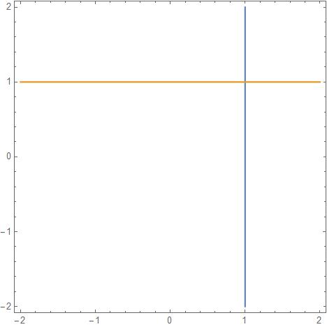
E.1.2 The Airy function

A slightly less trivial example is the Airy action

\displaystyle Z_{\lambda}=\int_{-\infty}^{\infty}\text{d}xe^{S}\,,\quad S=\text{i}\lambda\left(\frac{x^{3}}{3}-x\right)\ .

(684)

It is not hard to find that for real $\lambda$ there are three “convergent” regions, namely $\Re(S)<\infty$ , on the complex $x$ -plane:

\displaystyle x=re^{\text{i}\theta},\quad\frac{2n\pi}{3}\leq\theta\leq\frac{\pi}{3}+\frac{2n\pi}{3},\quad n=0,1,2.

(685)

In each convergent region, the Airy integrand is exponentially small. As we vary $\lambda$ to complex values, we should deform the integration contour of $x$ accordingly so that the integral remains converge. This gives an analytic continuation of $Z_{\lambda}$ . The two critical points are located at $x=\pm 1$ . The values of saddle points are

\displaystyle S_{\pm}=\mp\frac{2\text{i}\lambda}{3}.

(686)

Since along the (anti-)thimbles, the imaginary part of $S$ is a constant and

\displaystyle\text{Im}(S_{\pm})=\mp\frac{2\text{Re}(\lambda)}{3}.

(687)

Therefore the two (anti-)thimbles associated with the two critical points will not intersect except for the case of $\text{Re}(\lambda)=0$ . The thimble which connects critical points is called the Stoke ray. Using the Lefschetz thimbles $\mathcal{J}_{\pm}$ , we can rewrite the integral as

\displaystyle Z_{\lambda}=n_{+}\int_{\mathcal{J}_{+}}\exp S+n_{-}\int_{\mathcal{J}_{-}}\exp S.

(688)

To solve the thimbles, let us take $\lambda=1$ , then the flow equations are

\displaystyle\frac{\text{d}x}{\text{d}t}=\text{i}(\bar{x}^{2}-1).

(689)

Expressing $x=x_{1}+\text{i}x_{2}$ , we obtain

\displaystyle\frac{\text{d}x_{1}}{\text{d}t}=2x_{1}x_{2},\quad\frac{\text{d}x_{2}}{\text{d}t}=x_{1}^{2}-x_{2}^{2}-1.

(690)

We plot the anti-thimbles in Fig. 15

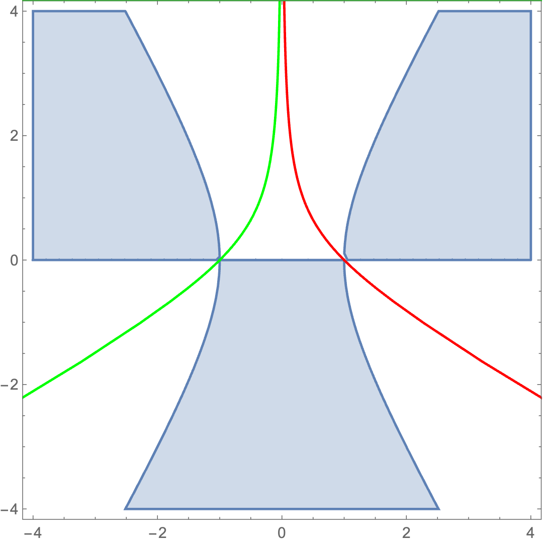
Therefore for $\lambda=1$ both of the saddle points contribute. This result is expected since that the two critical points are already located on the real line.

The problem we met in the main text is better illustrated by the following toy model

\displaystyle\tilde{Z}=\int_{-\infty}^{\infty}\text{d}x\exp S,\quad S=\text{i}\left(\frac{x^{3}}{3}+x\right)\ .

(691)

The integral is convergent and can be expressed by the Airy function

\displaystyle\tilde{Z}=\frac{2\pi\text{Ai}\left(\frac{1}{\sqrt[3]{3}}\right)}{\sqrt[3]{3}}=0.83\ .

(692)

We now try to compute the integral with saddle point approximation, where the saddle points are located at $x=\pm\text{i}$ . The saddle point value, plus the 1-loop correction, of the integral at these two saddle points, $\tilde{Z}_{\pm}$ are the same, and the sum of them is larger than the exact evaluation of the integral

\displaystyle\tilde{Z}_{+}=\tilde{Z}_{-}=0.733,\quad\tilde{Z}_{+}+\tilde{Z}_{-}>\tilde{Z}.

(693)

This is exactly the situation we are encountering. In this toy model, it is easy to show that the anti-thimble associated with the saddle point $x=-\text{i}$ does not intersect with the real axis, Figure. 16, so the saddle point $x=-\text{i}$ does not contribute to the integral.

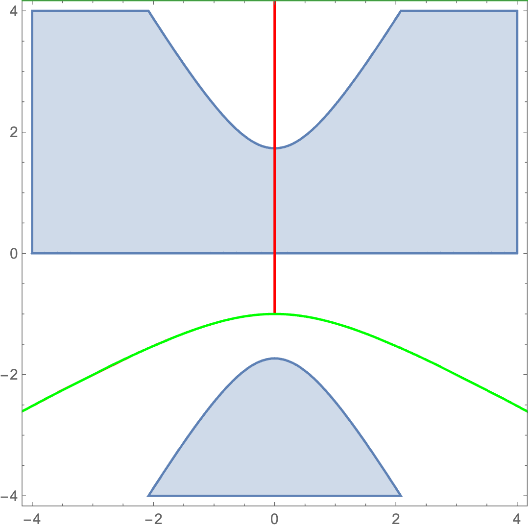
E.2 Multi-variable cases

Let us consider another example with two variables

\displaystyle Z=\int\text{d}\sigma\frac{\text{d}g}{2\pi}e^{S}\,,\quad S=\log\sigma-\text{i}\sigma g-\frac{1}{2}g^{2}\ .

(694)

The integral can be done directly to get

\displaystyle Z=0\ .

(695)

There are two saddle points

\displaystyle g_{\pm}=\pm\text{i},\quad\sigma_{\pm}=\mp 1\ .

(696)

with saddle point contributions to the integral (on-shell action)

\displaystyle Z_{\pm}=\mp\frac{1}{\sqrt{e}},\quad Z_{-}+Z_{+}=0\ ,

(697)

Matching this with the exact solution suggests that $n_{\pm}=1$ . Note that $\sigma_{\pm}=\mp 1$ are already on the real line so corresponding anti-thimbles always intersect with the original contour. The flow equations are

\displaystyle\frac{d\sigma}{dt}=-\frac{1}{\bar{\sigma}}-\text{i}\bar{g},\quad\frac{\text{d}g}{dt}=-\text{i}\bar{\sigma}+\bar{g}.

(698)

Expressing $\sigma=\sigma_{1}+\text{i}\sigma_{2}$ and $g=g_{1}+\text{i}g_{2}$ we obtain the following differential equations

	$\displaystyle\frac{\text{d}\sigma_{1}}{\text{d}t}+g_{2}+\frac{\sigma_{1}}{\sigma_{1}^{2}+\sigma_{2}^{2}}=0,\quad\frac{\text{d}\sigma_{2}}{\text{d}t}+g_{1}+\frac{\sigma_{2}}{\sigma_{1}^{2}+\sigma_{2}^{2}}=0,$		(699)
	$\displaystyle\frac{\text{d}g_{1}}{\text{d}t}+\sigma_{2}-g_{1}=0,\quad\frac{\text{d}g_{2}}{\text{d}t}+\sigma_{1}+g_{2}=0.$		(700)

We find that indeed these two saddles should both be included. We plot the $g$ -plane of the anti-thimbles in Fig. 17.

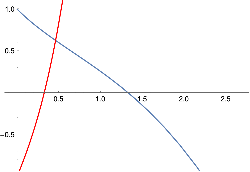
Note that this example is special case of (172) with $q=2$ .

Flow equations in real coordinates

Sometimes it more convenient to use real form of the flow equations (669). We start with the relations

\displaystyle\frac{\partial S}{\partial z}=\frac{1}{2}\frac{\partial S}{\partial x}+\frac{1}{2\text{i}}\frac{\partial S}{\partial y},

(701)

\displaystyle\frac{\partial\bar{S}}{\partial\bar{z}}=\frac{1}{2}\frac{\partial\bar{S}}{\partial x}-\frac{1}{2\text{i}}\frac{\partial\bar{S}}{\partial y},

(702)

where

\displaystyle z=x+\text{i}y.

(703)

Then we evaluate the equation as

\displaystyle\frac{\text{d}z}{\text{d}t}+\frac{\text{d}\bar{z}}{\text{d}t}

\displaystyle=-\frac{\partial S}{\partial z}-\frac{\partial\bar{S}}{\partial\bar{z}}=-\frac{\partial\text{Re}(S)}{\partial x}-\frac{\partial\text{Im}(S)}{\partial y},

(704)

\displaystyle\frac{\text{d}z}{\text{d}t}-\frac{\text{d}\bar{z}}{\text{d}t}

\displaystyle=\frac{\partial S}{\partial z}-\frac{\partial\bar{S}}{\partial\bar{z}}=-\text{i}\frac{\partial\text{Re}(S)}{\partial y}+\text{i}\frac{\partial\text{Im}(S)}{\partial x},

(705)

where we work in the flat space. Recall the Cauchy-Riemann equation we get

\displaystyle\frac{\text{d}x}{\text{d}t}=-\frac{\partial\text{Re}(S)}{\partial x},\quad\frac{\text{d}y}{\text{d}t}=-\frac{\partial\text{Re}(S)}{\partial y}.

(706)

To illustrate it we consider a special case in the Airy function

\displaystyle S=\text{i}\left(\frac{x^{3}}{3}+x\right).

(707)

In the complex plane its conjugate is

\displaystyle\bar{S}=-\text{i}\left(\frac{\bar{x}^{3}}{3}+\bar{x}\right),

(708)

and we can define the components

\displaystyle x=x_{1}+\text{i}x_{2},\quad\bar{x}=x_{1}-\text{i}x_{2}.

(709)

The flow equation in complex coordinates becomes

\displaystyle\frac{\text{d}x}{\text{d}t}=-\frac{\partial\bar{S}}{\partial\bar{x}}=\text{i}(\bar{x}^{2}+1),

(710)

which leads to the equations in real coordinates

\displaystyle\frac{\text{d}x_{1}}{\text{d}t}=2x_{1}x_{2},\quad\frac{\text{d}x_{2}}{\text{d}t}=x_{1}^{2}-x_{2}^{2}+1.

(711)

On the other hand we can get the equations with the real part of $S$ :

\displaystyle\text{Re}(S)=-x_{2}-x_{1}^{2}x_{2}+\frac{x_{2}^{3}}{3}.

(712)

From the equations (706) we can recover the two flow equations (711).

Appendix F Averaged models

In this section, before talking about higher dimensional model we detour the main topic a little bit and consider the averaged theory in general. Let us consider a real scalar field with a chemical potential. The partition function of the theory is

\displaystyle Z=\int{\cal D}\Phi\exp\left(-\int dx\,\partial_{\mu}\phi(x)\partial^{\mu}\phi(x)+J(x)\phi(x)\right)\,

(713)

where $J(x)$ is a random source drawn from some probability distribution. If the random coupling $J$ does not depends on the spacetime i.e.

\displaystyle\langle J^{n}\rangle_{\text{connected}}=\kappa_{n}\,\quad

(714)

where $\kappa_{n}$ is the $n$ -th cumulants of the probability distribution. This situation is like the regular SYK theory. To take the ensemble average we can expand the exponential as

	$\displaystyle\langle Z\rangle_{J}$	$\displaystyle=$	$\displaystyle\int{\cal D}\Phi\exp\left(-\int dx\,{\cal L}_{0}\right)\sum_{n}\frac{\langle J^{n}\rangle}{n!}\left(\int dx\,\phi(x)\right)^{n}$		(715)
		$\displaystyle=$	$\displaystyle\int{\cal D}\Phi\exp\left(-\int dx\,{\cal L}_{0}\right)\text{MGF}\left(\int dx\phi(x)\right)$		(716)

where MGF is the moment generating function of $J$ . If $J$ is Gaussian ${\cal N}(0,t^{2})$ then

	$\displaystyle\text{MGF}\left(\int dx\phi(x)\right)=\exp\left(\frac{t^{2}}{2}\int dx\,dy\,\phi(x)\phi(y)\right),$		(717)
	$\displaystyle\langle Z\rangle_{J}=\int{\cal D}\Phi\exp\left(-\int dx\,{\cal L}_{0}+\frac{t^{2}}{2}\int dx\,dy\,\phi(x)\phi(y)\right)\,$		(718)

which is similar to SYK model that after the Gaussian average, bi-local interaction is generated. For the general distribution (714), the resulting averaged action is

\displaystyle\langle Z\rangle_{J}=\int{\cal D}\Phi\exp\left(-\int dx\,{\cal L}_{0}+\sum_{n}\frac{\kappa_{n}}{n!}[\int dx\phi(x)]^{n}\right)\,,

(719)

so multi-local interactions will be generated. In particular, if the distribution is Poisson we have

\displaystyle\langle Z\rangle_{J}=\int{\cal D}\Phi\exp\left(-\int dx\,{\cal L}_{0}+e^{\lambda\int dx\phi(x)}-1\right)\,,

(720)

which is a highly non-local theory.

Alternatively we can require the random coupling $J$ to depend on the spacetime i.e.

\displaystyle\langle\prod^{n}_{i}J(x_{i})\rangle=\prod_{i=1,j=i}^{n}\delta(x_{i}-x_{j})\kappa_{n}\,.

(721)

This situation is like the Brownian SYK theory Saad:2018bqo . Now we can take the ensemble average to get

$\displaystyle\langle Z\rangle_{J}$	$\displaystyle=$	$\displaystyle\int{\cal D}\Phi\exp\left(-\int dx\,{\cal L}_{0}\right)\sum_{n}\frac{\langle J^{n}\rangle}{n!}\left(\int dx\,\phi(x)\right)^{n}$
	$\displaystyle=$	$\displaystyle\int{\cal D}\Phi\exp\left(-\int dx\,{\cal L}_{0}\right)\sum_{n}\frac{\kappa_{n}}{n!}\left(\int dx\,\phi^{n}(x)\right)$
	$\displaystyle=$	$\displaystyle\int{\cal D}\Phi\exp\left(-\int dx\,{\cal L}_{0}\right)\int dx\,\text{MGF}(\phi(x)).$	(723)

If $J$ is Gaussian ${\cal N}(0,t^{2})$ then we have

\displaystyle\langle Z\rangle_{J}=\int{\cal D}\Phi\exp\left(-\int dx\,({\cal L}_{0}+\frac{t^{2}}{2}\phi^{2}(x))\right).

(724)

and if $J$ is Poisson then we simply get

\displaystyle\langle Z\rangle_{J}=\int{\cal D}\Phi\exp\left(-\int dx\,[{\cal L}_{0}+\lambda(e^{\phi(x)}-1)]\right),

(725)

which also coincides with results in Peng:2020rno .

Appendix G Computations in large N

CLT with $\mu=0$

In the appendix, we will consider the half-wormhole conjecture for statistical model in a more systematic way. The error functions we care about are

	Error	$\displaystyle=Y^{2}-\langle Y^{2}\rangle+\langle Y\rangle^{2}-\Phi,$		(726)
	$\displaystyle\langle\text{Error}^{2}\rangle$	$\displaystyle=\langle\left(Y^{2}-\langle Y^{2}\rangle+\langle Y\rangle^{2}-\Phi\right)^{2}\rangle,$		(727)

where $\Phi$ is defined in (63). And if the approximation is proper we must have

\displaystyle\langle\text{Error}\rangle=0,\quad\langle\text{Error}^{2}\rangle/\langle Y^{4}\rangle\ll 1.

(728)

The first requirement leads to

\displaystyle\langle\Phi\rangle=\langle Y\rangle^{2}

(729)

which is proved around (63), then we have

\displaystyle\langle\text{Error}^{2}\rangle=\langle\left(Y^{2}+\langle Y\rangle^{2}-\Phi\right)^{2}\rangle-\langle Y^{2}\rangle^{2}.

(730)

In the following we’ll give one type of function and try to explore the feasibility of the proposal, i.e. we compute the two error functions and check the relations (728) respectively.

First we consider the function $Y$ consisting of $N$ identical and independent variables $X_{i}$ as

\displaystyle Y=\sum_{i\neq j}X_{i}X_{j},

(731)

and for simplicity each combination only appears once since $X_{i}$ ’s commute with each other. The properties for $X_{i}$ in this section are set as

\displaystyle\langle X\rangle=0,\quad\langle X^{2}\rangle=t^{2},

(732)

in the next section we’ll consider the distribution with a non-zero mean. But actually for any distribution the property (732) can always be satisfied since we can always take the subtraction

\displaystyle\tilde{X}=X-\langle X\rangle.

(733)

therefore our discussion may be applied into the case with any distribution.

Obviously the first requirement in (728) is satisfied then we consider the computation for the second requirement

\displaystyle Y^{2}=\sum_{i\neq j}X_{i}^{2}X_{j}^{2}+2\sum_{i\neq j\neq k}X^{2}_{i}X_{j}X_{k}+6\sum_{i\neq j\neq k\neq l}X_{i}X_{j}X_{k}X_{l},

(734)

where the first sum contains $p$ different terms

\displaystyle p={N\choose 2},

(735)

while we have $2p(N-2)/2$ for the second sum and $p(p-2(N-2)-1)/6$ for the third one. For the $\Phi$ in the approximation we have

	$\displaystyle\Phi$	$\displaystyle=\frac{1}{(2\pi)^{N}}\int d\vec{k}\frac{e^{-\text{i}\vec{k}\vec{X}}}{P(\vec{X})}\langle e^{\text{i}\vec{k}\vec{x}}\rangle\left(\frac{\langle Ye^{\text{i}\vec{k}\vec{x}}\rangle}{\langle e^{\text{i}\vec{k}\vec{x}}\rangle}\right)^{2},$		(736)
		$\displaystyle=\frac{1}{(2\pi)^{N}}\int d\vec{k}\frac{e^{-\text{i}\vec{k}\vec{X}}}{P(\vec{X})}\langle e^{\text{i}\vec{k}\vec{x}}\rangle\left(\sum_{i\neq j}\frac{\langle x_{i}x_{j}e^{\text{i}\vec{k}\vec{x}}\rangle}{\langle e^{\text{i}\vec{k}\vec{x}}\rangle}\right)^{2},$		(737)

the computation is similar to that in $Y^{2}$ so that we can split the $\Phi$ function into three parts according to the three sums in (734)

	$\displaystyle\Phi_{0}$	$\displaystyle=\frac{2}{(2\pi)^{N}}\int d\vec{k}\frac{e^{-\text{i}\vec{k}\vec{X}}}{P(\vec{X})}\langle e^{\text{i}\vec{k}\vec{x}}\rangle\sum_{i\neq j}\frac{\langle x_{i}x_{j}e^{\text{i}\vec{k}\vec{x}}\rangle}{\langle e^{\text{i}\vec{k}\vec{x}}\rangle}\frac{\langle x_{i}x_{j}e^{\text{i}\vec{k}\vec{x}}\rangle}{\langle e^{\text{i}\vec{k}\vec{x}}\rangle},$		(738)
		$\displaystyle=\sum_{i\neq j}\frac{1}{\left(2\pi\right)^{2}}\int dk_{i}dk_{j}\frac{e^{-\text{i}k_{i}X_{i}}e^{-\text{i}k_{j}X_{j}}}{P(X_{i})P(X_{j})}\langle e^{\text{i}k_{i}x_{i}}\rangle\langle e^{\text{i}k_{j}x_{j}}\rangle\left(\frac{\langle x_{i}e^{\text{i}k_{i}x_{i}}\rangle}{\langle e^{\text{i}k_{i}x_{i}}\rangle}\right)^{2}\left(\frac{\langle x_{j}e^{\text{i}k_{j}x_{j}}\rangle}{\langle e^{\text{i}k_{j}x_{j}}\rangle}\right)^{2},$		(739)

	$\displaystyle\Phi_{1}$	$\displaystyle=\frac{2}{(2\pi)^{N}}\int d\vec{k}\frac{e^{-\text{i}\vec{k}\vec{X}}}{P(\vec{X})}\langle e^{\text{i}\vec{k}\vec{x}}\rangle\sum_{i\neq j\neq k}\frac{\langle x_{i}x_{j}e^{\text{i}\vec{k}\vec{x}}\rangle}{\langle e^{\text{i}\vec{k}\vec{x}}\rangle}\frac{\langle x_{i}x_{k}e^{\text{i}\vec{k}\vec{x}}\rangle}{\langle e^{\text{i}\vec{k}\vec{x}}\rangle},$		(740)
		$\displaystyle=2\sum_{i\neq j\neq k}X_{j}X_{k}\frac{1}{2\pi}\int dk_{i}\frac{e^{-\text{i}k_{i}X_{i}}}{P(X_{i})}\langle e^{\text{i}k_{i}x_{i}}\rangle\left(\frac{\langle x_{i}e^{\text{i}k_{i}x_{i}}\rangle}{\langle e^{\text{i}k_{i}x_{i}}\rangle}\right)^{2},$		(741)

	$\displaystyle\Phi_{2}$	$\displaystyle=\frac{6}{(2\pi)^{N}}\int d\vec{k}\frac{e^{-\text{i}\vec{k}\vec{X}}}{P(\vec{X})}\langle e^{\text{i}\vec{k}\vec{x}}\rangle\sum_{i\neq j\neq k\neq l}\frac{\langle x_{i}x_{j}e^{\text{i}\vec{k}\vec{x}}\rangle}{\langle e^{\text{i}\vec{k}\vec{x}}\rangle}\frac{\langle x_{k}x_{l}e^{\text{i}\vec{k}\vec{x}}\rangle}{\langle e^{\text{i}\vec{k}\vec{x}}\rangle},$		(742)
		$\displaystyle=6\sum_{i\neq j\neq k\neq l}X_{i}X_{j}X_{k}X_{l}.$		(743)

For simplicity we can define the function below

\displaystyle\phi_{i}=\frac{1}{2\pi}\int dk\frac{e^{-\text{i}kX_{i}}}{P(X_{i})}\langle e^{\text{i}kx}\rangle\left(\frac{\langle xe^{\text{i}kx}\rangle}{\langle e^{\text{i}kx}\rangle}\right)^{2},

(744)

so that the $\Phi$ functions can be expressed as

\displaystyle\Phi_{0}=\sum_{i\neq j}\phi_{i}\phi_{j},

(745)

\displaystyle\Phi_{1}=2\sum_{i\neq j\neq k}\phi_{i}X_{j}X_{k}.

(746)

And note that the $\phi$ function has the property

\displaystyle\langle\phi_{i}\rangle=\langle X_{i}\rangle^{2},

(747)

which is useful in the later computation, where $X_{i}$ ’s are identical.

Then following the procedure we have

	$\displaystyle\langle\text{Error}^{2}\rangle$	$\displaystyle=\langle\left(Y^{2}+\langle Y\rangle^{2}-\Phi\right)^{2}\rangle-\langle Y^{2}\rangle^{2},$		(748)
		$\displaystyle=\left\langle\left(\sum_{i\neq j}\left(X_{i}^{2}X_{j}^{2}-\phi_{i}\phi_{j}\right)+2\sum_{i\neq j\neq k}\left(X^{2}_{i}-\phi_{i}\right)X_{j}X_{k}\right)^{2}\right\rangle-p^{2}\langle X^{2}\rangle^{4},$		(749)

where the last sum cancels out and $p$ is defined in (735). The cross terms between different sums are zero due to the zero mean of $X_{i}$ , therefore we can only consider the squares of each sum

\displaystyle\langle\text{Error}^{2}\rangle=\left\langle\left(\sum_{i\neq j}\left(X_{i}^{2}X_{j}^{2}-\phi_{i}\phi_{j}\right)\right)^{2}+\left(2\sum_{i\neq j\neq k}\left(X^{2}_{i}-\phi_{i}\right)X_{j}X_{k}\right)^{2}\right\rangle-p^{2}\langle X^{2}\rangle^{4}.

(750)

The numbers of the diagonal terms in the two sums in the first average are

\displaystyle p,\quad 4p(N-2),

(751)

while the non-diagonal terms in the first sum have

	$\displaystyle p(p-2(N-2)-1)\quad\text{ for }\quad\langle X_{i}^{2}X_{j}^{2}X_{k}^{2}X_{l}^{2}\rangle$		(752)
	$\displaystyle 2p(N-2)\quad\text{ for }\quad\langle X_{i}^{4}X_{j}^{2}X_{k}^{2}\rangle,$		(753)

and the non-diagonal terms in the second sum vanish due to the zero mean of $X_{i}$ .

We want to talk about (728) in this case, and the $\phi$ function has its role in the discussion. If the function $\phi$ satisfies the relation

\displaystyle X_{i}^{2}-\phi_{i}=f(X_{i}),\quad\langle f(X_{i})\rangle=0

(754)

where $f(X_{i})$ is an unknown function of $X_{i}$ . Actually this relation leads to

\displaystyle t^{2}=\langle X_{i}^{2}-\phi_{i}\rangle=0,

(755)

therefore in this case the distribution should be non-trivial with $\mu=0$ and $t=0$ . Usually we do not consider such cases, but we can still show how it works following this computation. Then in this case the dominant terms in $\langle\text{Error}^{2}\rangle$ will be (752) as it contains the largest number of terms. The $\phi$ terms are not included since the averages of the non-diagonal $\phi$ terms are zero because of (732) and (747). Then we can find that the dominant terms of $\langle\text{Error}^{2}\rangle$ which locate at the order $p^{2}$ or $N^{4}$ cancel out in (750). Therefore the relation (728) is satisfied since the dominant terms in $Y^{2}$ are also at the order $N^{4}$ , so that the proposal holds in this case when $N$ is sufficiently large.

While if $\phi$ has the relation below like what we have in the Gaussian case

\displaystyle X_{i}^{2}-\phi_{i}=g(X_{i}),\quad\langle g(X_{i})\rangle\neq 0

(756)

where $g(X_{i})$ is also unknown and we denote the average with a nonzero constant $C$ . Then the diagonal terms in the second sum can contribute to the dominant terms. We can have the explicit computation as the following,

\displaystyle 2\sum_{i\neq j\neq k}\left(X^{2}_{i}-\phi_{i}\right)X_{j}X_{k}\sim 2(N-2)C\sum_{j\neq k}X_{j}X_{k},

(757)

where the approximation is valid as we only care about the maximal numbers. In the square this term is similar to (734) except we have an extra parameter $4(N-2)^{2}$ . The non-vanishing contribution after the average will be the diagonal terms in the square as $X_{i}$ has a zero mean, which means the number of the terms is

\displaystyle 4(N-2)^{2}p=2N(N-1)(N-2)^{2}.

(758)

This contribution also locate at the order $N^{4}$ which is additional comparing to the previous case, so that the dominant terms can not cancel out in (750). Therefore the proposal fails in this case.

After having discussed a simple example We can try to consider the general one

\displaystyle Y=\sum_{i_{1}\dots i_{q}}X_{i_{1}}\dots X_{i_{q}},

(759)

where the sum contains $p$ terms

\displaystyle p={N\choose q}

(760)

and $X_{i}$ ’s are still identical and independent variables. Following the procedure above we have

\displaystyle Y^{2}=\sum_{i_{1}\dots i_{q}}X_{i_{1}}^{2}\dots X_{i_{q}}^{2}+\sum_{i_{1}\dots i_{q+1}}X_{i_{1}}^{2}\dots X_{i_{q-1}}^{2}X_{i_{q}}X_{i_{q+1}}+\dots+\sum_{i_{1}\dots i_{2q}}X_{i_{1}}\dots X_{i_{2q}},

(761)

the numbers of the total terms for each sum are respectively

\displaystyle{N\choose q},\quad{N\choose q}{q\choose 1}{N-q\choose 1},\dots,{N\choose q}{N-q\choose q},

(762)

and the numbers for each single term in each sum or the repetitions are

\displaystyle 1,\quad{2\choose 1},\quad{4\choose 2},\dots,{2q\choose q}.

(763)

When $q=2$ we can find that the computations in the two cases match. For the function $\Phi$ similarly we can define the functions

\displaystyle\Phi_{0},\quad\Phi_{1},\dots,\Phi_{q},

(764)

which correspond to the terms in (761) respectively. And we can also introduce the $\phi$ functions to express each $\Phi_{s}$ , substituting the $X^{2}_{i}$ by $\phi_{i}$ in (761) we can get all the $\Phi_{s}$ ’s just like (745),(746).

Following the previous procedure the square of the error function can be evaluated as

$\displaystyle\langle\text{Error}^{2}\rangle$	$\displaystyle=\langle\left(Y^{2}+\langle Y\rangle^{2}-\Phi\right)^{2}\rangle-\langle Y^{2}\rangle^{2},$	(765)
	$\displaystyle=\left\langle\left(\sum_{s=0}^{q}\sum_{i_{1}\dots i_{q+s}}\left(Y^{2}_{s}-\Phi_{s}\right)\right)^{2}\right\rangle-p^{2}\langle X^{2}\rangle^{2q},$	(766)
	$\displaystyle=\left\langle\sum_{s=0}^{q}\left(\sum_{i_{1}\dots i_{q+s}}\left(Y^{2}_{s}-\Phi_{s}\right)\right)^{2}\right\rangle-p^{2}\langle X^{2}\rangle^{2q},$	(767)

where the index $s$ labels the components in both $Y^{2}$ , $\Phi$ and the cross terms among the different sums vanish due to zero mean of $X_{i}$ .

Then we’ll encounter the previous problem again that there are two different conditions (754),(756) for $\phi$ , and we also first consider the former one. The total numbers of the diagonal terms in the above each sum $s$ are respectively

\displaystyle{N\choose q},\quad{2\choose 1}{N\choose q}{q\choose 1}{N-q\choose 1},\dots,{2(q-1)\choose q-1}{N\choose q}{q\choose q-1}{N-q\choose q-1},

(768)

which are the combinations of (762) and (763) and the last one in (761) cancels out. While about the non-diagonal terms as the averages of $X_{i}$ is zero, the nonzero non-diagonal terms only appears in the sum $s=0$ . And as the average of $\Phi_{i}$ is also zero, the nonzero non-diagonal terms in the sum $s=0$ will only come from $Y^{2}_{0}$ . The computation of the square of this term is similar to (761) except the replacement of $X_{i}$ by $X_{i}^{2}$ ,

\displaystyle Y^{4}_{nn}=\sum_{i_{1}\dots i_{q+1}}X_{i_{1}}^{4}\dots X_{i_{q-1}}^{4}X_{i_{q}}^{2}X_{i_{q+1}}^{2}+\dots+\sum_{i_{1}\dots i_{2q}}X_{i_{1}}^{2}\dots X_{i_{2q}}^{2},

(769)

where $nn$ means nonzero non-diagonal. The non-zero contributions in (767) come from the square of the first sum $s=0$ and the diagonal terms in the square of the other sums $s>0$ . And note that the last one labelled by $s=q$ cancels out, and in (768) the last one is subordinate to the square of the first term when $N$ , $q$ , $N/q$ are sufficiently large. Then under the condition (754) the dominant terms will be the first sum with square according to the equation (768). The square of the first sum in (767) gives the dominant terms which are the last one in (769), it contains the number

\displaystyle{N\choose q}{N-q\choose q}.

(770)

Then after the average the dominant terms in the square of the error becomes

\displaystyle\langle\text{Error}^{2}\rangle=\left({N\choose q}{N-q\choose q}-{N\choose q}{N\choose q}\right)\langle X^{2}\rangle^{2q},

(771)

which is subordinate comparing to $\langle Y^{4}\rangle$ .

While under the condition (756) the diagonal terms in the squares of the sums with $s>0$ will contribute. The computation is similar to the previous case with $q=2$ , the nonzero average increases the number of the diagonal or nonzero terms. As an example we calculate the last non-zero one in (767)

\displaystyle\sum_{ji_{1}\dots i_{2q-2}}(X_{j}^{2}-\phi_{j})X_{i_{1}}\dots X_{i_{2q-2}}=\alpha\sum_{i_{1}\dots i_{2q-2}}X_{i_{1}}\dots X_{i_{2q-2}}

(772)

where

\displaystyle\alpha=C{N\choose q}{q\choose q-1}{N-q\choose q-1}/{N\choose 2q-2},

(773)

and for simplicity we denote the $\phi$ term with $C$ . Since we only care about the number of the terms, the denotation does not matter for the result. The constant $C$ is defined in (756) and the numerator is the number of the terms in the sum labelled by $s=q-1$ , while the denominator is the number of the sum of the right hand side of (772). In the square of this term only the diagonal ones survive in the average, we have the number

\displaystyle{N\choose q}^{2}{q\choose q-1}^{2}{N-q\choose q-1}^{2}/{N\choose 2q-2}\sim N^{2q}\sim p^{2}.

(774)

Actually we can find that except the last sum all the sums in (767) will contribute to the dominant terms. So that the proposal will fail as the first sum cancels out with the last one in (767), while we have other additional contributions to the dominant terms.

CLT with $\mu\neq 0$

In the above section we have discussed the case with $\mu=0$ , after that we can move to consider the case with $\mu\neq 0$ . Remember that for the distribution with a non-zero mean we deal it with the subtraction (733), now we keep this non-trivial mean. The difference between them may be illustrated by a simple example

	$\displaystyle Y=\sum_{i\neq j}\left(X_{i}-\langle X_{i}\rangle\right)\left(X_{j}-\langle X_{j}\rangle\right),$		(775)
	$\displaystyle Y=\sum_{i\neq j}X_{i}X_{j}-\left\langle\sum_{i\neq j}X_{i}X_{j}\right\rangle.$		(776)

The two definitions are not equivalent which is manifest in the higher powers of $Y$ . Actually the former one is equivalent to the case with $\mu=0$ in the previous section, the latter without the subtraction is what we’ll consider in this section.

We still start with the simple case with $q=2$

	$\displaystyle Y=\sum_{i\neq j}X_{i}X_{j},$		(777)
	$\displaystyle Y^{2}=\sum_{i\neq j}X_{i}^{2}X_{j}^{2}+2\sum_{i\neq j\neq k}X^{2}_{i}X_{j}X_{k}+6\sum_{i\neq j\neq k\neq l}X_{i}X_{j}X_{k}X_{l}.$		(778)

About $\Phi$ we can have similar definition to (736), and the definition and the requirement for the error are the same as before. We also separate each sum in both $Y^{2}$ and $\Phi$ so that the square of the error can be expressed as

	$\displaystyle\langle\text{Error}^{2}\rangle$	$\displaystyle=\langle\left(Y^{2}+\langle Y\rangle^{2}-\Phi\right)^{2}\rangle-\langle Y^{2}\rangle^{2},$		(779)
		$\displaystyle=\left\langle\left(Y_{0}^{2}+\langle Y\rangle^{2}_{0}-\Phi_{0}+Y_{1}^{2}+\langle Y\rangle^{2}_{1}-\Phi_{1}\right)^{2}\right\rangle-\langle Y^{2}\rangle^{2}.$		(780)

And note that here we can not separate the square of the sum into the sum of the square of each sum, since now the cross terms are not zero due to the nonzero mean of $X_{i}$ . When $N\to\infty$ we can only consider the dominant terms, but as the case is different to before the terms we want will also be different. Now the dominant terms in the two parts in (780) are both in the second sum in (778) or $Y_{1}^{2}$ (780), since this sum contains the largest number of terms and is non-zero under the averagre because of the non-zero mean. Which means we can only consider the cross terms in the square of this sum which contains the largest number of terms. By the direct calculation we have

\displaystyle\Phi_{1}=2\sum_{i\neq j\neq k}\phi_{i}X_{j}X_{k},

(781)

where $\phi$ is defined in (744). Then we have

\displaystyle Y_{1}^{2}+\langle Y\rangle^{2}_{1}-\Phi_{1}=2\sum_{i\neq j\neq k}\left(\left(X_{i}^{2}-\phi_{i}\right)X_{j}X_{k}+\langle X_{i}\rangle^{2}\langle X_{j}\rangle\langle X_{k}\rangle\right),

(782)

while the dominant terms can be written as

\displaystyle\langle\text{Error}^{2}\rangle_{d}=\left\langle\left(2\sum_{i\neq j\neq k}\left(\left(X_{i}^{2}-\phi_{i}\right)X_{j}X_{k}+\langle X_{i}\rangle^{2}\langle X_{j}\rangle\langle X_{k}\rangle\right)\right)^{2}\right\rangle-\left\langle 2\sum_{i\neq j\neq k}X_{i}^{2}X_{j}X_{k}\right\rangle^{2}.

(783)

The dominant terms of the first part are the cross terms, whose number is at the same order of $N$ as the second part. So to evaluate the approximation we can only consider the two terms below

\displaystyle\langle\left(X_{i}^{2}-\phi_{i}\right)X_{j}X_{k}+\langle X_{i}\rangle^{2}\langle X_{j}\rangle\langle X_{k}\rangle\rangle,\quad\langle X_{i}^{2}X_{j}X_{k}\rangle,

(784)

where the variables are identical and independent. Recall that we have the equation (747) therefore the two expressions are equal under the average. Explicitly the cross terms also contain many parts, we can also write down the one with the largest number of terms,

\displaystyle\left(X_{i}^{2}-\phi_{i}\right)X_{j}X_{k}\left(X_{l}^{2}-\phi_{l}\right)X_{m}X_{n},\quad 4{N\choose 2}(N-2){N-3\choose 2}(N-5),

(785)

while the second part in (783) contains

\displaystyle 4{N\choose 2}^{2}(N-2)^{2}.

(786)

Therefore the dominant contribution in (783) will cancel out, which makes the proposal hold.

We can also consider the problem that occurs in the case with $\mu=0$ when the average of $X^{2}-\phi$ is not zero, and we can find that there’s no such problem here. As the dominant term (783) contains the largest number of $X$ terms, therefore even when $X^{2}-\phi$ is a constant the total number of $X$ terms in (783) will not change.

Next we consider the case with general $q$ . Following the previous procedure for the error we can get an expression similar to (780)

\displaystyle\langle\text{Error}^{2}\rangle=\left\langle\left(\sum_{s=0}^{q-1}(Y_{s}^{2}+\langle Y\rangle^{2}_{s}-\Phi_{s})\right)^{2}\right\rangle-\langle Y^{2}\rangle^{2},

(787)

and the dominant sum will also be the last non-zero one, i.e. the sum labelled with $s=q-1$ . To find out the behavior of the dominant terms the relation of the two functions below is important,

\displaystyle\langle\left(X_{i_{1}}^{2}-\phi_{i_{1}}\right)X_{i_{2}}\dots X_{i_{2q-1}}+\langle X_{i_{1}}\rangle^{2}\langle X_{i_{2}}\rangle\dots\langle X_{i_{2q-1}}\rangle\rangle,\quad\langle X_{i_{1}}^{2}X_{i_{2}}\dots X_{i_{2q-1}}\rangle,

(788)

we want to determine whether they are equal. And we can find that the relation (747) still holds thus the approximation is also proper in general $q$ .

SYK with one time point with $\mu=0$

Like in the previous section given any distribution we can always construct a variable with zero mean, such as

\displaystyle\tilde{X}=X-\langle X\rangle,

(789)

so that we can consider any distribution we want.

We first consider a simple case with $q=2$ , the Hamiltonian has the form

\displaystyle Y=\sum_{i\neq j}\text{sgn}(ij)X_{i}X_{j},

(790)

where $X_{i}$ ’s are identical and independent variables and the sign term mimics the sign function in the SYK model. Note that here we have no need to compute the explicit form of the sign function, since it has no effect yet. It is very similar to the previous case, but the difference is that here all $X_{i}$ ’s only appear once in the sum. Therefore for the square we have

\displaystyle Y^{2}=\sum_{i\neq j}X_{i}^{2}X_{j}^{2}+2\sum_{i\neq j\neq k\neq l}\text{sgn}(ijkl)X_{i}X_{j}X_{k}X_{l},

(791)

comparing to (734) it lacks the middle term. Our previous computation shows that the approximation fails in the Gaussian case with $\mu=0$ due to the middle term, thus the approximation is proper in this case no matter what the distribution is.

We can have an explicit computation for the proposal, but first the convention needs to be consistent with the SYK model. Now the total number $N$ counts the whole Majorana fermions and the number $q$ is for the number of the fermions in the interaction. Then for $N/q=2$ the expression (790) is still valid for the partition function, except that the $N$ and $q$ have different meanings. Then the number of $X_{i}$ in (790) becomes

\displaystyle\frac{N!}{\left(\left(N/2\right)!\right)^{2}},

(792)

and the sum contains the number of the terms

\displaystyle\frac{N!}{2!\left(\left(N/2\right)!\right)^{2}}.

(793)

Following the previous process we have

\displaystyle Y^{2}-\Phi=\sum_{i\neq j}\left(X_{i}^{2}X_{j}^{2}-\phi_{i}\phi_{j}\right)

(794)

where $\phi$ is defined in (744) and for the error

\displaystyle\langle\text{Error}^{2}\rangle=\left\langle\left(\sum_{i\neq j}\left(X_{i}^{2}X_{j}^{2}-\phi_{i}\phi_{j}\right)\right)^{2}\right\rangle-\left\langle\sum_{i\neq j}X_{i}^{2}X_{j}^{2}\right\rangle^{2}.

(795)

Since there are only two parts in the above function and the sums are the same, we can only compare the two expressions in the brackets. The average of $\phi$ is zero due to the zero mean of $X_{i}$ , so the proposal holds in the case. Explicitly the dominant terms in (795) come from the cross term in the first part and the whole second part, the number becomes

\displaystyle\frac{N!}{2!\left(\left(N/2\right)!\right)^{2}}\left(\frac{N!}{2!\left(\left(N/2\right)!\right)^{2}}-1\right)-\left(\frac{N!}{2!\left(\left(N/2\right)!\right)^{2}}\right)^{2}.

(796)

We can find the dominant terms cancel out so that the proposal is valid in this simple case.

Then we can consider a more general Hamiltonian with arbitrary $N$ and $q$ . Here we take the more familiar convention in SYK and still define $p=N/q$ , then the partition function becomes

\displaystyle z=\sum_{A}\text{sgn}(A)J_{A_{1}}\dots J_{A_{p}}.

(797)

Before we check the approximation we can first have some computation about the numbers of the different terms in this partition function. The total number of the $J_{A}$ ’s is

\displaystyle{N\choose q},

(798)

and the number of the combinations of $J_{A}$ ’s is

\displaystyle\frac{N!}{p!(q!)^{p}},

(799)

while the times for a single $J_{A}$ appearing in the Hamiltonian is

\displaystyle\frac{(N-q)!}{(p-1)!(q!)^{p-1}}.

(800)

The square of the partition function can be given as

	$\displaystyle z^{2}$	$\displaystyle=\sum_{A}\text{sgn}(A)^{2}J_{A_{1}}^{2}\dots J_{A_{p}}^{2}+\sum_{A,B}\text{sgn}(A)\text{sgn}(B)J_{A_{1}}^{2}\dots J_{A_{p-2}}^{2}J_{A_{p-1}}J_{A_{p}}J_{B_{p-1}}J_{B_{p}}$
		$\displaystyle\quad+\dots+\sum_{A,B}\text{sgn}(A)\text{sgn}(B)J_{A_{1}}\dots J_{A_{p}}J_{B_{1}}\dots J_{B_{p}}$		(801)

the first non-diagonal term appears with four different $J_{A}$ ’s as the combination $A$ should be the permutation of $1,\dots,N$ . And in the sums there may be many identical terms, here we may not give the explicit forms. To figure out the explicit expressions for the numbers in each sum we can count the numbers of different combinations of $r$ different $J_{A}$ ’s in the product of the combinations of $A$ and $B$ . Obviously there’s only one combination in the case $r=1$ , actually $r=1$ is identical to $r=0$ since the last $J_{A_{i}}$ in a combination $A$ can be determined by the other $p-1$ $J_{A_{i}}$ ’s. For the larger $r$ we have to subtract the combinations in $r-i$ $(i<r)$ to get the correct ones, as it can give $r-i$ cases in the product of two combinations. Therefore we have

	$\displaystyle r=2,\quad\frac{(2q)!}{2!(q!)^{2}}-1,$		(802)
	$\displaystyle r=3,\quad\frac{(3q)!}{3!(q!)^{3}}-{3\choose 2}\left(\frac{(2q)!}{2!(q!)^{2}}-1\right)-1,$		(803)

from the above we can introduce the function $n_{r}$ for this counting

\displaystyle n_{r}=\frac{(rq)!}{r!(q!)^{r}}-\sum_{s=2}^{r-1}{r\choose s}n_{s}-1.

(804)

From the calculation we can take mathematical induction to derive a simpler form

\displaystyle n_{r}=\sum_{s=1}^{r}\frac{(sq)!}{s!(q!)^{s}}{r\choose s}(-1)^{r-s}+(-1)^{r},\quad r>1,

(805)

and

\displaystyle n_{0}=1,

(806)

where $n_{1}$ is absent according to the equation (801).

Then we calculate the numbers of the terms in the each sum in (801),

\displaystyle\frac{N!}{p!(q!)^{p}}n_{0},\frac{N!}{p!(q!)^{p}}{p\choose 2}n_{2},\frac{N!}{p!(q!)^{p}}{p\choose 3}n_{3},\dots,\frac{N!}{p!(q!)^{p}}n_{p},

(807)

and note that the first one is different to the others. And about the last one the dominant term of the subtrahend should be at the order $(N-q)!$ , therefore the subtrahend is almost at the order $N(N-q)!$ . Actually this number is far larger than the accurate one, since in (805) there’s a factor $(-1)^{r-s}$ then the accurate number is approximately at $(N-q)!$ .

Here we also have two conditions similar to (754),(756), and first we consider the former one. As in this section we assume the mean of the $J_{A_{i}}$ is zero, therefore we have

\displaystyle\langle z^{2}\rangle=\left\langle\sum_{A}\text{sgn}(A)^{2}J_{A_{1}}^{2}\dots J_{A_{p}}^{2}\right\rangle=\frac{N!}{p!(q!)^{p}}\bar{J}^{2p}

(808)

where

\displaystyle\langle J_{A_{i}}^{2}\rangle=\bar{J}^{2}.

(809)

For the error we evaluate it as

	$\displaystyle\langle\text{Error}^{2}\rangle$	$\displaystyle=\langle\left(z^{2}-\Phi\right)^{2}\rangle-\langle z^{2}\rangle^{2},$		(810)
		$\displaystyle=\left\langle\sum_{s=0,2}^{p}\left(\sum_{i_{1}\dots i_{q+s}}\left(z^{2}_{s}-\Phi_{s}\right)\right)^{2}\right\rangle-\langle z^{2}\rangle^{2},$		(811)

where $s$ does not take value $1$ for clarity and the cross terms of different sums are zero due to the zero mean of $J_{A_{i}}$ . Then we find that the computation is similar to before that for $s>0$ the nonzero contribution under the average is the diagonal terms in the square, while for $s=0$ the whole terms contribute to the computation of the error. Which means to find out the dominant sum $s$ we should compare the square of the first term with the rest terms in (807), and note that the last one cancels out in (811) so that the non-trivial largest number should be the one labeled by $p-1$ . And we give an upper bound for it

\displaystyle\frac{N!}{p!(q!)^{p}}{p\choose p-1}n_{p-1}<p^{2}\frac{N!}{p!(q!)^{p}}\frac{(N-q)!}{(p-1)!(q!)^{p-1}}.

(812)

Note that the number of the identical terms in this sum may have an effect but we expect the upper bound is still valid. Then we can find that when $N$ , $q$ are sufficiently large it is subordinate to the square of the first term in (807). Therefore we write the dominant terms in (811)

\displaystyle\frac{N!}{p!(q!)^{p}}n_{p}-\left(\frac{N!}{p!(q!)^{p}}\right)^{2}

(813)

where the cross terms of the first part and the whole second part contribute. Recall the expression (805) the dominant terms in the above equation cancel out, which implies the proposal holds.

Then we consider the second condition (756) that for a single variable we can view $J_{A_{i}}^{2}-\Phi_{i}$ as a constant. The expression (811) is still valid so that the thing we need to consider is to find the correction to (813). As an example we consider the behavior of the second sum labeled by $s=2$ , the diagonal contribution after the subtraction should be

\displaystyle\alpha\sum J_{A_{p-1}}J_{A_{p}}J_{B_{p-1}}J_{B_{p}},

(814)

where $\alpha$ is determined by the quotient of the two numbers of the two sum

\displaystyle\alpha=\frac{N!}{p!(q!)^{p}}{p\choose 2}n_{2}/\left({N\choose 2q}\frac{(2q)!}{2!(q!)^{2}}n_{2}\right).

(815)

Therefore after the square the total number becomes

\displaystyle\left(\frac{N!}{p!(q!)^{p}}{p\choose 2}n_{2}\right)^{2}/\left({N\choose 2q}\frac{(2q)!}{2!(q!)^{2}}n_{2}\right),

(816)

comparing to the two terms in (813) the above term is subordinate. Similarly we can find that after the subtraction the largest number in the sums $s>0$ occurs in the case $s=p-1$ , which gives

\displaystyle\left(\frac{N!}{p!(q!)^{p}}{p\choose p-1}n_{p-1}\right)^{2}/\left({N\choose N-q}\frac{(N-q)!}{(p-1)!(q!)^{p-1}}n_{p-1}\right).

(817)

The above contribution is still subordinate to the two terms in (813), which means the proposal is proper in this case.

Thus for the SYK model we can conclude that when the mean is zero the proposal works well no matter what the distribution is.

SYK with one time point with $\mu\neq 0$

Like what we have discussed before the case with non-zero mean is different to last section. The whole computation is similar to the case with $\mu=0$ except the mean terms, we can take relevant expressions from the previous sections. We consider the case with general $N/q$ ,

\displaystyle z=\sum_{A}\text{sgn}(A)J_{A_{1}}\dots J_{A_{p}},

(818)

the main task here is find the dominant terms. The sign functions may have some effect which makes $s=q-1$ not dominant, such as when $N/q$ =2 we have

\displaystyle\left\langle\sum_{A}\text{sgn}(A)J_{A_{1}}J_{A_{2}}\right\rangle=\sum_{A}\text{sgn}(A)\langle J_{A_{i}}\rangle^{2}={N/2-1\choose[N/4]}\langle J_{A_{i}}\rangle^{2},

(819)

where the square bracket means the integer part. Actually here $N/4$ is $q/2$ , in the later computation we always have even $q$ therefore we’ll omit the square bracket.

To derive this parameter explicitly we have two different ways, one is to find the sequence functions over different $N$ which can be solved by Mathematica. Another is to consider different combinations, we can define the positive and the negative combinations then their difference gives the parameter. Given $N$ different numbers we can have a permutation group which can be divided into the even and odd parts, and the two parts contain the same number of elements. If the indices of $J$ have no order then the numbers of the even and odd parts are equal, so that the parameter is zero. But in the SYK model the indices are listed in a particular order, it makes the numbers of the two parts different.

To proceed the computation we define the sign of a $q$ -sequence,

\displaystyle\text{sgn}(J_{A_{i}})=(-1)^{a_{i_{1}}+\dots+a_{i_{q}}},\quad q=0\text{mod}(4)

(820)

where when $q=2\text{mod}(4)$ the sign will be opposite. Note that here we take the $a_{i}$ from the indices of $J_{A_{i}}$ , but what in the superscript should be the initial sites of the indices. When the indices take the values $1,\dots,N$ , the values themselves naturally label their initial sites. But when the indices take arbitrary numbers or symbols, we can define an initial order and the sites with any permutation. After the assignment complete we can take the definition (820) to define the sign of any given $q$ -sequence.

Then for a combination $A$ containing $r$ negative q-sequences we have the argument

\displaystyle\text{sgn}(A)=1,\quad\text{if }\sum_{i=1}^{r}s_{i}=0\text{mod}(2),

(821)

where $s_{i}$ is the site of the $i$ -th negative $q$ -sequence. We give the condition above as the negative $q$ -sequences seems appearing in pairs. For $N/q=2$ the positive combination $A$ contains two positive q-sequences, so our mission is to find the first sequence with positive sign. As the combination has an order the first index in $J_{A_{1}}$ is 1, we only need to consider the others. The positive $q$ -sequence has the number

\displaystyle{N/2-1\choose 1}{N/2\choose q-2}+{N/2-1\choose 3}{N/2\choose q-4}+\dots+{N/2-1\choose q-1}{N/2\choose 0},

(822)

where $q=N/2$ the first chooses odd number of odd integers while the second chooses even number of even integers. Then the negative $q$ -sequence has

\displaystyle{N/2-1\choose 0}{N/2\choose q-1}+{N/2-1\choose 2}{N/2\choose q-3}+\dots+{N/2-1\choose q-2}{N/2\choose 1},

(823)

the difference of the two numbers will give the parameter

\displaystyle d(p,q)=\sum_{i=0}^{q-1}(-1)^{i+1}{pq/2-1\choose i}{pq/2\choose q-1-i},

(824)

which coincides with (819) when $N/q=2$ . For general $p=N/q$ we can also find an expression for finding the first positive $q$ -sequence

\displaystyle d(p,q)=\frac{1}{p-1}{pq/2-1\choose q/2},

(825)

where $q$ is even and it can be verified by numerics.

And note that for different $q$ ’s there may be a difference with the minus sign, which is explained in (820).

For general $N/q$ we can try to compute $\gamma$ in the expression below by the recursion

\displaystyle\left\langle\sum_{A}\text{sgn}(A)J_{A_{1}}\dots J_{A_{p}}\right\rangle=\sum_{A}\text{sgn}(A)\langle J_{A_{i}}\rangle^{p}=\gamma\langle J_{A_{i}}\rangle^{p}.

(826)

In the previous computation we have calculated the case with $p=2$ , we only need to derive the $p+1$ case from the $p$ one. Given $N$ numbers we can give the difference between the positive combinations and the negative ones which is denoted as $D(p,q)$ and we have

\displaystyle D(2,q)=d(2,q),\quad D(p+1)=f(D(p,q)).

(827)

where $f$ is an unknown function. When we add extra $q$ numbers to the $N$ case which is already known, in the new permutation we can fix one number in the extra $q$ ones at the $p+1$ site in case of repetition. For simplicity we let the additional $q$ numbers be $1,\dots,q$ and put it at the first site, and we always fix the number $1$ in this site.

We determine the first site through the procedure in the case of $p=2$ , which can be divided into the positive and negative parts. After choosing $q$ numbers from the $N+q$ ones, about the left $N$ numbers we assume we already know the difference between the positive combinations and the negative ones. To illustrate the product of the sequences, we define the positive (negative) sequences as $P_{+}$ ( $P_{-}$ ) so that we have

\displaystyle P_{+}P_{+}=P_{+},\quad P_{-}P_{-}=P_{+},\quad P_{+}P_{-}=P_{-}.

(828)

The product of two positive or two negative sequences gives a positive one while the product of one positive and one negative sequences gives a negative one. Then we can derive the sequences in the case $N+q$ as

\displaystyle P_{+}^{N+q}=P^{q}_{+}P^{N}_{+}+P^{q}_{-}P^{N}_{-},\quad P_{-}^{N+q}=P^{q}_{+}P^{N}_{-}+P^{q}_{+}P^{N}_{-},

(829)

therefore the difference of the positive and negative sequences can be illustrated as

\displaystyle P_{+}^{N+q}-P_{-}^{N+q}=(P_{+}^{q}-P_{-}^{q})(P_{+}^{N}-P_{-}^{N}).

(830)

Which means the recursion can be expressed as

\displaystyle D(p,q)=d(p,q)D(p-1,q)=\prod_{s=2}^{p}d(s,q),

(831)

inserting the equation (825) it becomes

\displaystyle D(p,q)=\frac{(pq/2-1)!}{(p-1)!(q/2-1)!((q/2)!)^{p-1}}=\frac{(pq/2)!}{p!((q/2)!)^{p}}.

(832)

Then we can try to evaluate the cross terms in the square of the partition function (801). Consider the terms with $p-s$ squares in the sequence,

\displaystyle\sum_{A,B}\text{sgn}(A)\text{sgn}(B)J_{A_{1}}^{2}\dots J_{A_{p-s}}^{2}J_{A_{p-s+1}}\dots J_{A_{p}}J_{B_{p-s+1}}\dots J_{B_{p}},

(833)

after the average over $J$ the number in the sum becomes

\displaystyle d_{s}=\sum_{r=2}^{s}{p-r\choose s-r}{N\choose pq-rq}\frac{(pq-rq)!}{(p-r)!(q!)^{p-r}}D(r,q)^{2}(-1)^{s-r}+{p\choose s}(s-1)(-1)^{s-1}\frac{(pq)!}{p!(q!)^{p}},

(834)

where the derivation is similar to the equation (805).

We can find an upper bound for the number (834)

\displaystyle{N\choose pq-sq}\frac{(pq-sq)!}{(p-s)!(q!)^{p-s}}D(s,q)^{2},

(835)

Then for $s=2,\dots,p-1$ we can compare the above number to the first one in (807), from this we may find out the dominant one.

By a few numerical comparisons it seems that the dominant terms do not locate at a particular $s$ as the two parameters $p$ , $q$ vary. In this computation we can directly take the equation (834) rather than the one with approximation.

Appendix H Some details about the fermion integral

The relevant integral is

	$\displaystyle I_{f}^{N}$	$\displaystyle=$	$\displaystyle\int\text{d}^{2N}\psi\exp\left(T[\sum_{i}[\Sigma_{LR}\psi_{i}^{L}\psi_{i}^{R}+\Sigma_{L}\theta_{i}\psi_{i}^{L}+\Sigma_{R}\theta_{i}\psi_{i}^{R}]\right)\,$		(836)
		$\displaystyle=$	$\displaystyle\left(\int\text{d}\psi^{L}\text{d}\psi^{R}\exp(T\Sigma_{LR}\psi^{L}\psi^{R})\exp(T\Sigma_{L}\theta\psi^{L})\exp(T\Sigma_{R}\theta\psi^{R})\right)^{N}$		(837)

Before evaluating this integral we need some specifications. Here $\psi^{L(R)}$ are not Grassmann numbers but can be transferred into Dirac fermions as

	$\displaystyle c=\frac{\psi^{L}+\text{i}\psi^{R}}{2},\quad c^{\dagger}=\frac{\psi^{L}-\text{i}\psi^{R}}{2},\quad\psi_{L}=c+c^{\dagger},\quad\psi_{R}=\text{i}(c^{\dagger}-c)\,$		(838)
	$\displaystyle\{c,c^{\dagger}\}=1,\quad\{c,c\}=\{c^{\dagger},c^{\dagger}\}=0\,.$		(839)

Then the integral $I_{f}$ becomes

	$\displaystyle I_{f}$	$\displaystyle=$	$\displaystyle 2\int\text{d}c\text{d}c^{\dagger}e^{a_{1}(cc^{\dagger}-c^{\dagger}c)+a_{-}c+a_{+}c^{\dagger}},\quad a_{1}=\text{i}T\Sigma_{LR},\quad a_{\pm}=T(\Sigma_{L}\pm\text{i}\Sigma_{R})\theta,$		(840)
		$\displaystyle=$	$\displaystyle 4\cosh(\sqrt{a_{1}^{2}+a_{+}a_{-}})=4\cosh(T\sqrt{\Sigma_{L}^{2}+\Sigma_{R}^{2}-\Sigma_{LR}^{2}})$		(841)

Next let us use the same method to compute (382):

$\displaystyle I_{4}^{N}$	$\displaystyle=$	$\displaystyle\int\text{d}^{4N}\psi\exp\left(\Sigma_{ab}\psi_{i}^{a}\psi_{i}^{b}\right)$	(843)
	$\displaystyle=$	$\displaystyle\{\int\text{d}^{4}\psi\exp\left(\frac{1}{2}\Sigma_{12}\psi^{1}\psi^{2}+\Sigma_{13}\psi^{1}\psi^{3}+\Sigma_{14}\psi^{1}\psi^{4}\right.$
		$\displaystyle\quad\left.\Sigma_{23}\psi^{2}\psi^{3}+\Sigma_{24}\psi^{2}\psi^{4}+\Sigma_{34}\psi^{3}\psi^{4}\right)\}^{N}.$

Generally to compute $I_{4}$ let us introduce two Dirac fermions

\displaystyle\psi_{1}=\sqrt{h}(c_{1}+c_{1}^{\dagger}),\quad\psi_{2}=\text{i}\sqrt{h}(c_{1}-c_{1}^{\dagger}),\quad\psi_{3}=\sqrt{h}(c_{2}+c_{2}^{\dagger}),\quad\psi_{4}=\text{i}\sqrt{h}(c_{2}-c_{2}^{\dagger}),

(844)

such that $\Sigma_{ab}\psi_{i}^{a}\psi_{i}^{b}$ can be written as a $4\times 4$ matrix $H$ with non-vanishing elements

	$\displaystyle H_{11}=-\text{i}h(\Sigma_{12}+\Sigma_{34}),\quad H_{14}=-h(\Sigma_{13}-\Sigma_{24})-\text{i}h(\Sigma_{14}+\Sigma_{23})$		(845)
	$\displaystyle H_{22}=\text{i}h(\Sigma_{34}-\Sigma_{12}),\quad H_{23}=-h(\Sigma_{13}+\Sigma_{24})+\text{i}h(\Sigma_{14}-\Sigma_{23})$		(846)
	$\displaystyle H_{32}=h(\Sigma_{13}+\Sigma_{24})+\text{i}h(\Sigma_{14}-\Sigma_{23}),\quad H_{33}=-\text{i}h(\Sigma_{34}-\Sigma_{12})$		(847)
	$\displaystyle H_{41}=h(\Sigma_{13}-\Sigma_{24})-\text{i}h(\Sigma_{14}+\Sigma_{23}),\quad H_{44}=\text{i}h(\Sigma_{12}+\Sigma_{34}).$		(848)

By diagonalizing this matrix we can compute $I_{4}$ as the trace of the exponential of the matrix

	$\displaystyle I_{4}=2\left(\cos\left(h\sqrt{(\Sigma_{14}-\Sigma_{23})^{2}+(\Sigma_{13}+\Sigma_{24})^{2}+(\Sigma_{12}-\Sigma_{34})^{2}}\right)\right.$
	$\displaystyle\qquad\left.+\cos\left(h\sqrt{(\Sigma_{14}+\Sigma_{23})^{2}+(\Sigma_{13}-\Sigma_{24})^{2}+(\Sigma_{12}+\Sigma_{34})^{2}}\right)\right).$		(849)

And note that the change of the variable from $\psi$ to $c$ , $c^{\dagger}$ will introduce an additional coefficient in the integral

\displaystyle(2h)^{2},

(850)

the final result is the product of the two terms.

References

(1) J. M. Maldacena, “The Large N limit of superconformal field theories and supergravity,” Adv. Theor. Math. Phys. 2, 231-252 (1998) doi:10.1023/A:1026654312961 [arXiv:hep-th/9711200 [hep-th]].
(2) E. Witten, “Anti-de Sitter space and holography,” Adv. Theor. Math. Phys. 2, 253-291 (1998) doi:10.4310/ATMP.1998.v2.n2.a2 [arXiv:hep-th/9802150 [hep-th]].
(3) S. S. Gubser, I. R. Klebanov and A. M. Polyakov, “Gauge theory correlators from noncritical string theory,” Phys. Lett. B 428, 105-114 (1998) doi:10.1016/S0370-2693(98)00377-3 [arXiv:hep-th/9802109 [hep-th]].
(4) G. Penington, “Entanglement Wedge Reconstruction and the Information Paradox,” JHEP 09, 002 (2020) doi:10.1007/JHEP09(2020)002 [arXiv:1905.08255 [hep-th]].
(5) A. Almheiri, N. Engelhardt, D. Marolf and H. Maxfield, “The entropy of bulk quantum fields and the entanglement wedge of an evaporating black hole,” JHEP 12, 063 (2019) doi:10.1007/JHEP12(2019)063 [arXiv:1905.08762 [hep-th]].
(6) A. Almheiri, R. Mahajan, J. Maldacena and Y. Zhao, “The Page curve of Hawking radiation from semiclassical geometry,” JHEP 03, 149 (2020) doi:10.1007/JHEP03(2020)149 [arXiv:1908.10996 [hep-th]].
(7) G. Penington, S. H. Shenker, D. Stanford and Z. Yang, “Replica wormholes and the black hole interior,” [arXiv:1911.11977 [hep-th]].
(8) S. R. Coleman, “Black Holes as Red Herrings: Topological Fluctuations and the Loss of Quantum Coherence,” Nucl. Phys. B 307, 867-882 (1988) doi:10.1016/0550-3213(88)90110-1
(9) S. B. Giddings and A. Strominger, “Baby Universes, Third Quantization and the Cosmological Constant,” Nucl. Phys. B 321, 481-508 (1989) doi:10.1016/0550-3213(89)90353-2
(10) S. B. Giddings and A. Strominger, “Loss of Incoherence and Determination of Coupling Constants in Quantum Gravity,” Nucl. Phys. B 307, 854-866 (1988) doi:10.1016/0550-3213(88)90109-5
(11) J. Polchinski and A. Strominger, “A Possible resolution of the black hole information puzzle,” Phys. Rev. D 50, 7403-7409 (1994) doi:10.1103/PhysRevD.50.7403 [arXiv:hep-th/9407008 [hep-th]].
(12) P. Saad, S. H. Shenker and D. Stanford, “JT gravity as a matrix integral,” [arXiv:1903.11115 [hep-th]].
(13) P. Saad, S. H. Shenker and D. Stanford, “A semiclassical ramp in SYK and in gravity,” [arXiv:1806.06840 [hep-th]].
(14) P. Saad, “Late Time Correlation Functions, Baby Universes, and ETH in JT Gravity,” [arXiv:1910.10311 [hep-th]].
(15) C. Yan, “Crosscap Contribution to Late-Time Two-Point Correlators,” [arXiv:2203.14436 [hep-th]].
(16) R. Bousso, X. Dong, N. Engelhardt, T. Faulkner, T. Hartman, S. H. Shenker and D. Stanford, “Snowmass White Paper: Quantum Aspects of Black Holes and the Emergence of Spacetime,” [arXiv:2201.03096 [hep-th]].
(17) J. M. Maldacena and L. Maoz, “Wormholes in AdS,” JHEP 02, 053 (2004) doi:10.1088/1126-6708/2004/02/053 [arXiv:hep-th/0401024 [hep-th]].
(18) D. Stanford and E. Witten, “JT gravity and the ensembles of random matrix theory,” Adv. Theor. Math. Phys. 24, no.6, 1475-1680 (2020) doi:10.4310/ATMP.2020.v24.n6.a4 [arXiv:1907.03363 [hep-th]].
(19) L. V. Iliesiu, “On 2D gauge theories in Jackiw-Teitelboim gravity,” [arXiv:1909.05253 [hep-th]].
(20) D. Kapec, R. Mahajan and D. Stanford, “Matrix ensembles with global symmetries and ’t Hooft anomalies from 2d gauge theory,” JHEP 04, 186 (2020) doi:10.1007/JHEP04(2020)186 [arXiv:1912.12285 [hep-th]].
(21) H. Maxfield and G. J. Turiaci, “The path integral of 3D gravity near extremality; or, JT gravity with defects as a matrix integral,” JHEP 01, 118 (2021) doi:10.1007/JHEP01(2021)118 [arXiv:2006.11317 [hep-th]].
(22) E. Witten, “Matrix Models and Deformations of JT Gravity,” Proc. Roy. Soc. Lond. A 476, no.2244, 20200582 (2020) doi:10.1098/rspa.2020.0582 [arXiv:2006.13414 [hep-th]].
(23) E. Mefford and K. Suzuki, “Jackiw-Teitelboim quantum gravity with defects and the Aharonov-Bohm effect,” JHEP 05, 026 (2021) doi:10.1007/JHEP05(2021)026 [arXiv:2011.04695 [hep-th]].
(24) A. Altland and J. Sonner, “Late time physics of holographic quantum chaos,” SciPost Phys. 11, 034 (2021) doi:10.21468/SciPostPhys.11.2.034 [arXiv:2008.02271 [hep-th]].
(25) L. Eberhardt, “Summing over Geometries in String Theory,” JHEP 05, 233 (2021) doi:10.1007/JHEP05(2021)233 [arXiv:2102.12355 [hep-th]].
(26) D. Stanford, Z. Yang and S. Yao, “Subleading Weingartens,” JHEP 02, 200 (2022) doi:10.1007/JHEP02(2022)200 [arXiv:2107.10252 [hep-th]].
(27) I. Aref’eva and I. Volovich, “Gas of Baby Universes in JT Gravity and Matrix Models,” Symmetry 12, no.6, 975 (2020) doi:10.3390/sym12060975 [arXiv:1905.08207 [hep-th]].
(28) P. Betzios and O. Papadoulaki, “Liouville theory and Matrix models: A Wheeler DeWitt perspective,” JHEP 09, 125 (2020) doi:10.1007/JHEP09(2020)125 [arXiv:2004.00002 [hep-th]].
(29) D. Anninos and B. Mühlmann, “Notes on matrix models (matrix musings),” J. Stat. Mech. 2008, 083109 (2020) doi:10.1088/1742-5468/aba499 [arXiv:2004.01171 [hep-th]].
(30) M. Berkooz, V. Narovlansky and H. Raj, “Complex Sachdev-Ye-Kitaev model in the double scaling limit,” JHEP 02, 113 (2021) doi:10.1007/JHEP02(2021)113 [arXiv:2006.13983 [hep-th]].
(31) T. G. Mertens and G. J. Turiaci, “Liouville quantum gravity – holography, JT and matrices,” JHEP 01, 073 (2021) doi:10.1007/JHEP01(2021)073 [arXiv:2006.07072 [hep-th]].
(32) G. J. Turiaci, M. Usatyuk and W. W. Weng, “Dilaton-gravity, deformations of the minimal string, and matrix models,” doi:10.1088/1361-6382/ac25df [arXiv:2011.06038 [hep-th]].
(33) D. Anninos and B. Mühlmann, “Matrix integrals & finite holography,” JHEP 06, 120 (2021) doi:10.1007/JHEP06(2021)120 [arXiv:2012.05224 [hep-th]].
(34) P. Gao, D. L. Jafferis and D. K. Kolchmeyer, “An effective matrix model for dynamical end of the world branes in Jackiw-Teitelboim gravity,” [arXiv:2104.01184 [hep-th]].
(35) V. Godet and C. Marteau, “From black holes to baby universes in CGHS gravity,” JHEP 07, 138 (2021) doi:10.1007/JHEP07(2021)138 [arXiv:2103.13422 [hep-th]].
(36) C. V. Johnson, F. Rosso and A. Svesko, “Jackiw-Teitelboim supergravity as a double-cut matrix model,” Phys. Rev. D 104, no.8, 086019 (2021) doi:10.1103/PhysRevD.104.086019 [arXiv:2102.02227 [hep-th]].
(37) A. Blommaert and M. Usatyuk, “Microstructure in matrix elements,” [arXiv:2108.02210 [hep-th]].
(38) K. Okuyama and K. Sakai, “JT gravity, KdV equations and macroscopic loop operators,” JHEP 01, 156 (2020) doi:10.1007/JHEP01(2020)156 [arXiv:1911.01659 [hep-th]].
(39) S. Forste, H. Jockers, J. Kames-King and A. Kanargias, “Deformations of JT Gravity via Topological Gravity and Applications,” [arXiv:2107.02773 [hep-th]].
(40) A. Maloney and E. Witten, “Averaging over Narain moduli space,” JHEP 10, 187 (2020) doi:10.1007/JHEP10(2020)187 [arXiv:2006.04855 [hep-th]].
(41) N. Afkhami-Jeddi, H. Cohn, T. Hartman and A. Tajdini, “Free partition functions and an averaged holographic duality,” JHEP 01, 130 (2021) doi:10.1007/JHEP01(2021)130 [arXiv:2006.04839 [hep-th]].
(42) J. Cotler and K. Jensen, “AdS₃ gravity and random CFT,” JHEP 04, 033 (2021) doi:10.1007/JHEP04(2021)033 [arXiv:2006.08648 [hep-th]].
(43) A. Pérez and R. Troncoso, “Gravitational dual of averaged free CFT’s over the Narain lattice,” JHEP 11, 015 (2020) doi:10.1007/JHEP11(2020)015 [arXiv:2006.08216 [hep-th]].
(44) N. Benjamin, C. A. Keller, H. Ooguri and I. G. Zadeh, “Narain to Narnia,” Commun. Math. Phys. 390, no.1, 425-470 (2022) doi:10.1007/s00220-021-04211-x [arXiv:2103.15826 [hep-th]].
(45) J. Cotler and K. Jensen, “AdS₃ wormholes from a modular bootstrap,” JHEP 11, 058 (2020) doi:10.1007/JHEP11(2020)058 [arXiv:2007.15653 [hep-th]].
(46) M. Ashwinkumar, M. Dodelson, A. Kidambi, J. M. Leedom and M. Yamazaki, “Chern-Simons Invariants from Ensemble Averages,” doi:10.1007/JHEP08(2021)044 [arXiv:2104.14710 [hep-th]].
(47) N. Afkhami-Jeddi, A. Ashmore and C. Cordova, “Calabi-Yau CFTs and Random Matrices,” [arXiv:2107.11461 [hep-th]].
(48) S. Collier and A. Maloney, “Wormholes and Spectral Statistics in the Narain Ensemble,” [arXiv:2106.12760 [hep-th]].
(49) N. Benjamin, S. Collier, A. L. Fitzpatrick, A. Maloney and E. Perlmutter, “Harmonic analysis of 2d CFT partition functions,” doi:10.1007/JHEP09(2021)174 [arXiv:2107.10744 [hep-th]].
(50) J. Dong, T. Hartman and Y. Jiang, “Averaging over moduli in deformed WZW models,” doi:10.1007/JHEP09(2021)185 [arXiv:2105.12594 [hep-th]].
(51) A. Dymarsky and A. Shapere, “Comments on the holographic description of Narain theories,” JHEP 10, 197 (2021) doi:10.1007/JHEP10(2021)197 [arXiv:2012.15830 [hep-th]].
(52) V. Meruliya, S. Mukhi and P. Singh, “Poincaré Series, 3d Gravity and Averages of Rational CFT,” JHEP 04, 267 (2021) doi:10.1007/JHEP04(2021)267 [arXiv:2102.03136 [hep-th]].
(53) R. Bousso and E. Wildenhain, “Gravity/ensemble duality,” Phys. Rev. D 102, no.6, 066005 (2020) doi:10.1103/PhysRevD.102.066005 [arXiv:2006.16289 [hep-th]].
(54) O. Janssen, M. Mirbabayi and P. Zograf, “Gravity as an ensemble and the moment problem,” JHEP 06, 184 (2021) doi:10.1007/JHEP06(2021)184 [arXiv:2103.12078 [hep-th]].
(55) J. Cotler and K. Jensen, “Wormholes and black hole microstates in AdS/CFT,” JHEP 09, 001 (2021) doi:10.1007/JHEP09(2021)001 [arXiv:2104.00601 [hep-th]].
(56) D. Marolf and H. Maxfield, “Transcending the ensemble: baby universes, spacetime wormholes, and the order and disorder of black hole information,” JHEP 08, 044 (2020) doi:10.1007/JHEP08(2020)044 [arXiv:2002.08950 [hep-th]].
(57) V. Balasubramanian, A. Kar, S. F. Ross and T. Ugajin, “Spin structures and baby universes,” JHEP 09, 192 (2020) doi:10.1007/JHEP09(2020)192 [arXiv:2007.04333 [hep-th]].
(58) J. G. Gardiner and S. Megas, “2d TQFTs and baby universes,” JHEP 10, 052 (2021) doi:10.1007/JHEP10(2021)052 [arXiv:2011.06137 [hep-th]].
(59) A. Belin and J. de Boer, “Random statistics of OPE coefficients and Euclidean wormholes,” Class. Quant. Grav. 38, no.16, 164001 (2021) doi:10.1088/1361-6382/ac1082 [arXiv:2006.05499 [hep-th]].
(60) A. Belin, J. De Boer, P. Nayak and J. Sonner, “Charged Eigenstate Thermalization, Euclidean Wormholes and Global Symmetries in Quantum Gravity,” [arXiv:2012.07875 [hep-th]].
(61) A. Altland, D. Bagrets, P. Nayak, J. Sonner and M. Vielma, “From operator statistics to wormholes,” Phys. Rev. Res. 3, no.3, 033259 (2021) doi:10.1103/PhysRevResearch.3.033259 [arXiv:2105.12129 [hep-th]].
(62) A. Belin, J. de Boer, P. Nayak and J. Sonner, “Generalized Spectral Form Factors and the Statistics of Heavy Operators,” [arXiv:2111.06373 [hep-th]].
(63) C. Peng, J. Tian and J. Yu, “Baby universes, ensemble averages and factorizations with matters,” [arXiv:2111.14856 [hep-th]].
(64) A. Banerjee and G. W. Moore, “Comments on Summing over bordisms in TQFT,” [arXiv:2201.00903 [hep-th]].
(65) J. J. Heckman, A. P. Turner and X. Yu, “Disorder averaging and its UV discontents,” Phys. Rev. D 105, no.8, 086021 (2022) doi:10.1103/PhysRevD.105.086021 [arXiv:2111.06404 [hep-th]].
(66) C. V. Johnson, “The Microstate Physics of JT Gravity and Supergravity,” [arXiv:2201.11942 [hep-th]].
(67) S. Collier and E. Perlmutter, “Harnessing S-Duality in $\mathcal{N}=4$ SYM & Supergravity as $SL(2,\mathbb{Z})$ -Averaged Strings,” [arXiv:2201.05093 [hep-th]].
(68) J. Chandra, S. Collier, T. Hartman and A. Maloney, “Semiclassical 3D gravity as an average of large-c CFTs,” [arXiv:2203.06511 [hep-th]].
(69) J. M. Schlenker and E. Witten, “No Ensemble Averaging Below the Black Hole Threshold,” [arXiv:2202.01372 [hep-th]].
(70) R. Jackiw, “Lower Dimensional Gravity,” Nucl. Phys. B 252, 343-356 (1985) doi:10.1016/0550-3213(85)90448-1
(71) C. Teitelboim, “Gravitation and Hamiltonian Structure in Two Space-Time Dimensions,” Phys. Lett. B 126, 41-45 (1983) doi:10.1016/0370-2693(83)90012-6
(72) S. Sachdev and J. Ye, “Gapless spin fluid ground state in a random, quantum Heisenberg magnet,” Phys. Rev. Lett. 70, 3339 (1993) doi:10.1103/PhysRevLett.70.3339 [arXiv:cond-mat/9212030 [cond-mat]].
(73) A. Kitaev, ”A simple model of quantum holography.” Talks at KITP http://online.kitp.ucsb.edu/online/entangled15/kitaev/ and http://online.kitp.ucsb.edu/online/entangled15/kitaev2
A. Kitaev, ”Hidden correlations in the Hawking radiation and thermal noise.” Talk at KITP http://online.kitp.ucsb.edu/online/joint98/kitaev/
(74) D. Stanford, “More quantum noise from wormholes,” [arXiv:2008.08570 [hep-th]].
(75) A. Almheiri and H. W. Lin, “The Entanglement Wedge of Unknown Couplings,” [arXiv:2111.06298 [hep-th]].
(76) P. Saad, S. Shenker and S. Yao, “Comments on wormholes and factorization,” [arXiv:2107.13130 [hep-th]].
(77) P. Saad, S. H. Shenker, D. Stanford and S. Yao, “Wormholes without averaging,” [arXiv:2103.16754 [hep-th]].
(78) B. Mukhametzhanov, “Half-wormholes in SYK with one time point,” [arXiv:2105.08207 [hep-th]].
(79) A. M. García-García and V. Godet, “Half-wormholes in nearly AdS₂ holography,” [arXiv:2107.07720 [hep-th]].
(80) S. Choudhury and K. Shirish, “Wormhole calculus without averaging from $O(N)^{q-1}$ tensor model,” [arXiv:2106.14886 [hep-th]].
(81) B. Mukhametzhanov, “Factorization and complex couplings in SYK and in Matrix Models,” [arXiv:2110.06221 [hep-th]].
(82) K. Okuyama and K. Sakai, “FZZT branes in JT gravity and topological gravity,” JHEP 09, 191 (2021) doi:10.1007/JHEP09(2021)191 [arXiv:2108.03876 [hep-th]].
(83) K. Goto, Y. Kusuki, K. Tamaoka and T. Ugajin, “Product of random states and spatial (half-)wormholes,” JHEP 10, 205 (2021) doi:10.1007/JHEP10(2021)205 [arXiv:2108.08308 [hep-th]].
(84) A. Blommaert, L. V. Iliesiu and J. Kruthoff, “Gravity factorized,” [arXiv:2111.07863 [hep-th]].
(85) K. Goto, K. Suzuki and T. Ugajin, “Factorizing Wormholes in a Partially Disorder-Averaged SYK Model,” [arXiv:2111.11705 [hep-th]].
(86) A.I. Barvinok, New algorithms for linear k-matroid intersection and matroid k-parity problems, Mathematical Programming 69 (1995) 449A470.
(87) C. Peng, “Ensemble averages, Poisson processes, and microstates,” Phys. Rev. D 103, no.6, L061901 (2021) doi:10.1103/PhysRevD.103.L061901 [arXiv:2010.11192 [hep-th]].
(88) N. N. Bogolyubov, “On the theory of superfluidity,” J. Phys. (USSR) 11, 23-32 (1947) Valatin:1958ja
(89) J. G. Valatin, “Comments on the theory of superconductivity,” Nuovo Cim. 7, 843-857 (1958) doi:10.1007/BF02745589
(90) E. Witten, “Analytic Continuation Of Chern-Simons Theory,” AMS/IP Stud. Adv. Math. 50, 347-446 (2011) [arXiv:1001.2933 [hep-th]].
(91) A. Blommaert and J. Kruthoff, “Gravity without averaging,” [arXiv:2107.02178 [hep-th]].
(92) A. Blommaert, T. G. Mertens and H. Verschelde, “Eigenbranes in Jackiw-Teitelboim gravity,” JHEP 02, 168 (2021) doi:10.1007/JHEP02(2021)168 [arXiv:1911.11603 [hep-th]].
(93) A. Goel, L. V. Iliesiu, J. Kruthoff and Z. Yang, “Classifying boundary conditions in JT gravity: from energy-branes to $\alpha$ -branes,” JHEP 04, 069 (2021) doi:10.1007/JHEP04(2021)069 [arXiv:2010.12592 [hep-th]].
(94) A. Blommaert, L. V. Iliesiu and J. Kruthoff, “Alpha states demystified: Towards microscopic models of AdS₂ holography,” [arXiv:2203.07384 [hep-th]].
(95) D. Das, S. Pal and A. Sarkar, “(Half) Wormholes under Irrelevant Deformation,” [arXiv:2203.14988 [hep-th]].

Half-Wormholes and Ensemble Averages

Abstract

1 Introduction

1.1 Summary of our main results

2 Statistical models

2.1 Models of a single random variable

2.1.1 Recursion relations for approximations to arbitrary accuracy

2.1.2 Explicit relations for Gaussian approximation

2.2 Models with multiple independent identical random variables

2.2.1 Simple observables

2.2.2 Power-sum observables

2.2.3 Product observables

2.3 Large-NN constraints and half-wormhole approximation

2.3.1 Why and how to modify the approximation proposal

2.3.2 Why the proposal works for the Pfaffian in the SYK model

3 SYK at one time point: ⟨Ja⟩=0\langle J_{a}\rangle=0

3.1 SYK model with one time point

3.2 The saddle points analysis

3.2.1 The averaged ⟨z2⟩\langle z^{2}\rangle

3.2.2 The unaveraged z2z^{2}: the wormhole saddle

3.2.3 The unaveraged z2z^{2}: the linked half-wormhole saddles

4 SYK at one time point: ⟨Ja⟩≠0\langle J_{a}\rangle\neq 0

4.1 Half-wormhole saddle in zz

4.2 Linked half-wormhole saddles in z2z^{2}

5 SYK at one time point: ⟨Ja⟩=0,⟨Ja4⟩c≠0\langle J_{a}\rangle=0,\quad\langle J_{a}^{4}\rangle_{c}\neq 0

6 SYK at one time point: ⟨Ja⟩=⟨Ja2⟩=⟨Ja3⟩=0\langle J_{a}\rangle=\langle J_{a}^{2}\rangle=\langle J_{a}^{3}\rangle=0

6.1 Averaged quantities: ⟨z4⟩\langle z^{4}\rangle and ⟨z8⟩\langle z^{8}\rangle

6.2 The un-averaged z4z^{4}

7 SYK at one time point: Poisson distribution

8 The Brownian SYK model

8.1 ⟨|z|2⟩\langle|z|^{2}\rangle in the Brownian SYK model: accurate evaluation

8.2 ⟨|z|2⟩\langle|z|^{2}\rangle in the Brownian SYK model: large-NN saddle point evaluation

8.2.1 Saddle point solution: the q=1q=1 case

8.2.2 Saddle point solution: q>1q>1 at short time T​σ≪1T\sigma\ll 1

8.2.3 Long time T​σ≫1T\sigma\gg 1

8.3 ⟨|z|4⟩\langle|z|^{4}\rangle in the Brownian SYK model

8.3.1 Exact evaluation

8.3.2 Saddle point analysis

8.4 z2z^{2} at fixed coupling in the Brownian SYK model

8.4.1 Exact computation

8.4.2 Saddle point computation

Very short time

Short time

Long time

8.5 Half-wormholes

9 Modified Brownian SYK model

9.1 Brownian SYK with non-vanishing mean value

9.2 Random coupling from product of Grassmann variables JA(0)=J​∏iθAiJ_{A}^{(0)}=J\prod_{i}\theta_{A_{i}}

9.2.1 0d model

9.2.2 1d model

10 Discussion

Partially averaged models and spacetime branes

Standard SYK model

Non-trivial saddles and Null states

Acknowledgements.

Appendix A Explicit examples: simple observables

Appendix B Explicite Examples: composite observables

Gaussian distribution

Exponential distribution

Poisson distribution

Appendix C Explicte Examples: generalized statistical models

The exponential distribution

Poisson distribution

Appendix D Exact evaluation of ⟨z4⟩\langle z^{4}\rangle for Brownian SYK at large T

Appendix E Lefschetz Thimbles

E.1 some examples

E.1.1 The Gaussian function

E.1.2 The Airy function

E.2 Multi-variable cases

Flow equations in real coordinates

Appendix F Averaged models

Appendix G Computations in large N

CLT with μ=0\mu=0

CLT with μ≠0\mu\neq 0

SYK with one time point with μ=0\mu=0

SYK with one time point with μ≠0\mu\neq 0

Appendix H Some details about the fermion integral

References

2.3 Large- $N$ constraints and half-wormhole approximation

3 SYK at one time point: $\langle J_{a}\rangle=0$

3.2.1 The averaged $\langle z^{2}\rangle$

3.2.2 The unaveraged $z^{2}$ : the wormhole saddle

3.2.3 The unaveraged $z^{2}$ : the linked half-wormhole saddles

4 SYK at one time point: $\langle J_{a}\rangle\neq 0$

4.1 Half-wormhole saddle in $z$

4.2 Linked half-wormhole saddles in $z^{2}$

5 SYK at one time point: $\langle J_{a}\rangle=0,\quad\langle J_{a}^{4}\rangle_{c}\neq 0$

6 SYK at one time point: $\langle J_{a}\rangle=\langle J_{a}^{2}\rangle=\langle J_{a}^{3}\rangle=0$

6.1 Averaged quantities: $\langle z^{4}\rangle$ and $\langle z^{8}\rangle$

6.2 The un-averaged $z^{4}$

8.1 $\langle|z|^{2}\rangle$ in the Brownian SYK model: accurate evaluation

8.2 $\langle|z|^{2}\rangle$ in the Brownian SYK model: large- $N$ saddle point evaluation

8.2.1 Saddle point solution: the $q=1$ case

8.2.2 Saddle point solution: $q>1$ at short time $T\sigma\ll 1$

8.2.3 Long time $T\sigma\gg 1$

8.3 $\langle|z|^{4}\rangle$ in the Brownian SYK model

8.4 $z^{2}$ at fixed coupling in the Brownian SYK model

9.2 Random coupling from product of Grassmann variables $J_{A}^{(0)}=J\prod_{i}\theta_{A_{i}}$

Appendix D Exact evaluation of $\langle z^{4}\rangle$ for Brownian SYK at large T

CLT with $\mu=0$

CLT with $\mu\neq 0$

SYK with one time point with $\mu=0$

SYK with one time point with $\mu\neq 0$