=1pt
Hamiltonian cycles in annular decomposable Barnette graphs
Abstract
Barnette’s conjecture is an unsolved problem in graph theory. The problem states that every -regular (cubic), -connected, planar, bipartite (Barnette) graph is Hamiltonian. Partial results have been derived with restrictions on number of vertices, several properties of face-partitions and dual graphs of Barnette graphs while some studies focus just on structural characterizations of Barnette graphs. Noting that Spider web graphs are a subclass of Annular Decomposable Barnette (ADB graphs) graphs and are Hamiltonian, we study ADB graphs and their annular-connected subclass (ADB-AC graphs). We show that ADB-AC graphs can be generated from the smallest Barnette graph () using recursive edge operations. We derive several conditions assuring the existence of Hamiltonian cycles in ADB-AC graphs without imposing restrictions on number of vertices, face size or any other constraints on the face partitions. We show that there can be two types of annuli in ADB-AC graphs, ring annuli and block annuli. Our main result is, ADB-AC graphs having non singular sequences of ring annuli are Hamiltonian.
Keywords: Barnette conjecture, Hamiltonian graphs, Annular Decomposition, Planar cubic graphs, Bipartite polyhedral graphs
1 Introduction
Barnette’s conjecture is a long standing unsolved problem in mathematics proposed by David W. Barnette in 1969. The conjecture states:
Conjecture 1.1.
Every -regular, -connected planar bipartite graph is Hamiltonian. We will henceforth use the term Barnette graphs to refer to -regular, -connected planar bipartite graphs.
The development towards the Barnette’s conjecture started as early as 1880, when P.G. Tait proposed a weaker statement:
Conjecture 1.2.
Every -regular, -connected planar graph is Hamiltonian.
This conjecture was ultimately disproved by W.T. Tutte, when he constructed a couter-example to the conjecture, a graph built on vertices [13]. With further attempts to find a smaller counterexamples for Tait’s conjecture, Holton and McKay found a counterexample on vertices [8]. However, none of these counterexamples found were bipartite. Tutte thus proposed a conjecture stating:
Conjecture 1.3.
Every -regular, -connected bipartite graph is Hamiltonian.
Interestingly, a counterexample of this conjecture was found in 1976 by J.D. Horton which is a graph on vertices, known as the Horton graph [9]. The Barnette conjecture was thus proposed by combining Conjecture 1.2 and Conjecture 1.3 and remains unsolved.
There are several studies that addressed Conjecture 1.1. There have been attempts to understand the structure of Barnette graphs in general [3, 4]. One of the well known approaches is the proof by Holton, Manvel and McKay in 1984, showing that all -regular, -connected planar bipartite graphs with no more than 64 vertices are Hamiltonian [7]. In the same paper, they also present an interesting approach to generate all possible Barnette graphs from the smallest Barnette graphs, using simple operations defined by adding small structures to existing graphs. Other attempts have been made by studying the duals of Barnette graphs [11, 5, 1]. We conclude from the existing literature, that most of the studies, aiming to find Hamiltonian subclasses of Barnette graphs, focus on studying the dual graphs or imposing restriction on the faces of Barnette graphs.
In this article, we study properties of Annular Decomposable Barnette (ADB graphs) graphs, a sublclass of Barnette graphs. The idea of annular graphs is not novel in itself [2, 12]. Another article derives necessary and sufficient conditions when cubic plane graphs have a rectangular-radial drawing [6]. Interestingly, ADB graphs can be thought of as Barnette graphs that have a rectangular-radial drawing. One related work, that inspired us particularly to study ADB graphs in context to a Hamiltonian problem, is the result that Spider-web graphs have a Hamiltonian cycle excluding any edge in such graphs [10]. The Spider-web graphs can be characterised as ADB-graphs(see Figure 2) in [10]) and thus, can be viewed as a subclass of graphs we have studied. We show how Annular Decomposable Barnette Annular Connected (ADB-AC) graphs, a certain subclass of ADB-graphs can be built recursively from the smallest Barnette graph using edge operations. We derive some sufficient conditions under which, ADB-AC graphs are Hamiltonian. In our results we do not impose restrictions on number of vertices, face size or any other constraint on the face partitions. We show that there can be two types of annuli in ADB-AC graphs, ring annuli and block annuli. Our main result is, ADB-AC graphs having non singular sequences of ring annuli are Hamiltonian.
2 Preliminary definitions and notations
As per the Jordan curve theorem, a non-self-intersecting continuous loop in the 2-D plane has an interior and an exterior. For a planar embedding of a Barnette graph we can view a cycle or face, in as a Jordan curve and naturally induce a sense of interior, exterior and a boundary to . Note that a Hamiltonian cycle , if it exists, in a planar embedding of a Barnette graph would have the following properties:
-
1.
The interior of is path connected
-
2.
The exterior of is path connected
-
3.
All vertices in lie in the boundary of .
The idea is illustrated in Figure 1(a).
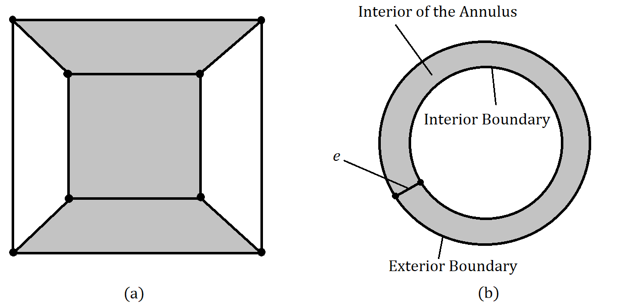
Note that, two non intersecting Jordan curves on a 2-D plane can always be drawn on the plane such that they are topologically equivalent to two non-intersecting concentric circles. We will refer to such a structure as an annulus (See Figure 1(b)). Intuitively, an annulus will have an interior and the exterior boundary once drawn on a plane as shown in Figure 1(b). The enclosed region between the two Jordan curves in a given planar projection of an annulus will be referred to as the interior of the annulus.
Definition 2.1.
We call a Barnette graph to be Annular Decomposable, if there exists a planar embedding of such that:
-
1.
can be partitioned into sequence of annuli
-
2.
The interior boundary of is a face called interior face
-
3.
The exterior boundary of is a face called exterior face
-
4.
Interior boundary of some annulus , , is the exterior boundary for some annulus
-
5.
Every edge in are such that, either and lie on the boundary of some annulus, or lies in outer boundary of some annulus and lies on the inner boundary of ().
If can be partitioned into annuli, we call an -Annular Decomposable Barnette (-ADB graph) graph.
Definition 2.2.
Let be a -ADB graph. If in a planar embedding of , , and are realized, we call it a planar annular embedding of .
Definition 2.3.
Let be a -ADB graph, . If for every annulus , , deleting all edges (along with respective vertices) in the interior of produces either two separate Barnette graphs or a Barnette graph and a vertex-less Jordan curve, then we call an ADB annular connected (-ADB-AC graph) graph.
In this article we prove that ADB-AC graphs having non singular sequences of ring annuli are Hamiltonian.
Lemma 2.4.
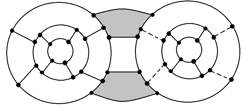
There exists ADB graphs that are not annular-connected.
Proof.
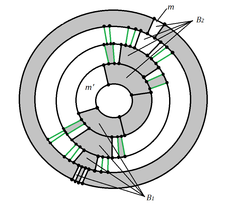
Let be an -ADB graph. Then be a copy of . Consider two consecutive edges and that lie in the interior of the outer annuals of , that are adjacent to vertices and of . Consider the two analogous edges and in , that are adjacent to vertices and of . Let and be the edges on the outer boundary of the outer annuli of and , connecting with and with respectively. Note that each of the four vertices, , , and , there is yet another edge adjacent to the vertices which we will denote as, , , and respectively. We now form a new graph by the following steps:
-
1.
Join and by drawing two edges across the existing edges
-
2.
Join and by drawing one edge across the existing edges
-
3.
Join and by drawing one edge across the existing edges
The resulting graph has annuli and it is easy to see that is an ADB graph, where is the number of annuli in . Note that can be viewed as a subgraph of . Now we delete all the edges in the interior of the outer annulus of , to obtain two graphs and with and annuli respectively. Note that, is not a Barnette graph since it is not bipartite. (See Figure 2) ∎
Definition 2.5.
Let be ADB-AC graph drawn on a plane. We denote the outer annulus of as .
Definition 2.6.
Let be ADB-AC graph drawn on a plane. Let have annuli. For some , we define the graph formed by considering restricting only until the -th annulus, to be the -annular restriction of , denoted by . Note that we clarify here that in , we do not consider any vertex adjacent to the edges in the interior of .
3 Main Results
Lemma 3.1.
Let be a Barnette graph. Then is 2-edge connected.
Proof.

Note that given a Hamiltonian Barnette Graph , if we apply the operation described in Figure 3(b), which we will henceforth call a -operation, any arbitrary number of times, the result is still a Hamiltonian graph. However, this is not true if we apply the operation described in Figure 3(a), which we will henceforth call a -operation, any arbitrary number of times. Later, in Theorem 3.6, we show that ADB-AC graphs can be constructed from by using arbitrary number of -operations only.
Lemma 3.2.
If every annulus of an ADB graph has a -Cycle, then is Hamiltonian. Note that this statement is true for any AD-Planar graph.
Proof.
Let us consider an ADB-AC graph . Let us consider the outer annulus of the graph . There are even number of faces in the outer annulus of since, the outer boundary of the outer annulus of , is an even cycle. Thus, the set of faces in the outer annulus of , denoted by can be partitioned into subsets and , such that no two faces in , are adjacent to each other.
Lemma 3.3.
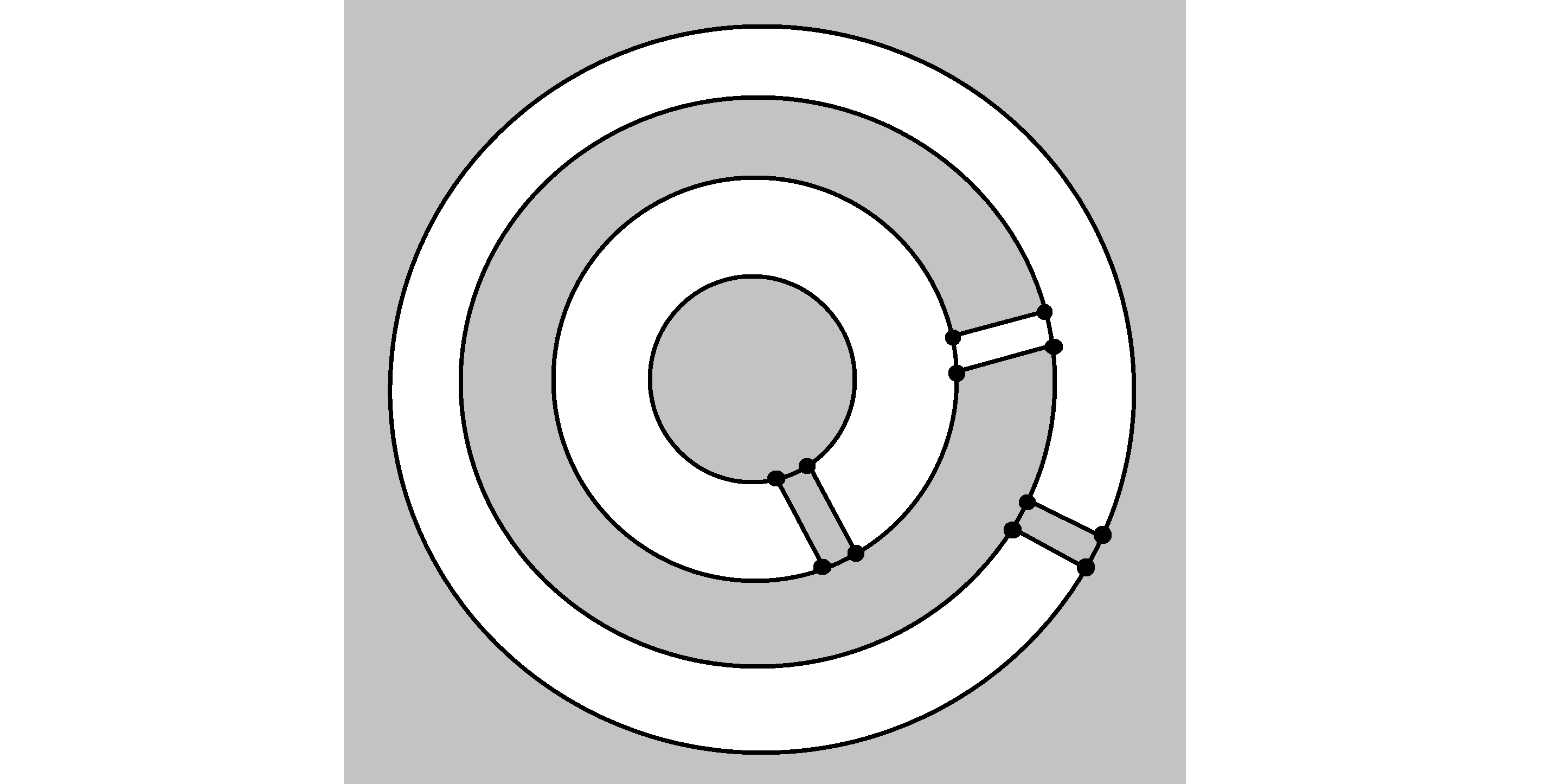
Let us consider an ADB-AC graph with annuli. Either or consists of only -cycles.
Proof.
Let us create a graph , by deleting all the edges in the interior of the outer annulus (along with their respective vertices). would be an ADB-AC graph, since is an ADB-AC graph. Thus, can be partitioned into subsets and , such that no two faces in , are adjacent to each other.
We claim that, the edges in the interior of the outer annulus of are all attached to the outer boundary of faces in , such that all such faces belong either in or in , but not both. To prove this claim, let us assume otherwise. Then, there exits two edges and in the interior of , such that is attached to the outer boundary of some face and is attached to some face . Let, and be the two vertices by which and are attached to the outer boundary of . Then there must be an odd number of vertices between and , considering the fact that and are in different partitions. Thus, there is an odd cycle in , which is impossible, since is bipartite.
Let us assume, without loss of generality, that all edges in interior of are attached to outer boundary of faces in . Note that for an arbitrary face , to which some of such edges are attached, we can assert that there are only even number of edges attached to , Otherwise, would transform into a odd cycle (face) in . Thus, there would always be a sequence of odd number of -cycles, (for some integer ) formed in adjacent to . Starting from , if we consider all alternate faces in , they will all be -cycles and will form a face partition of -cycles in . Thus the statement holds. ∎
As per convention, we will assume to be the face partition containing -cycles only in . Note here that, both the inner and outer annulus in any planar annular embedding of an -ADB graph must have at least two -cycles each. This along with Lemma 3.2 gives the following corollary.
Corollary 3.4.
Every -ADB graph is Hamiltonian.
Corollary 3.5.
Every be an -ADB graph. If there exists a planar annular projection of such that the -th annulus has more edges in its interior than the number of faces in the interior of the th annulus, then is Hamiltonian.
Proof.
The proof of this statement also follows from Lemma 3.2. Note that if there exists such a graph , then each of its annulus will have a -cycle. ∎
Theorem 3.6.
Let us consider an ADB-AC graph . Then can be constructed from by using arbitrary number of -operations only.
Proof.
Let have annuli for a particular planar annular embedding. For , the result is obviously true.
Recall that, as per our convention, the -face-only partition in the outer annulus of an ADB-AC graph is assumed to be . Let . By Lemma 3.3,say consists of only -cycles. Let us select any two such -cycles and . All other edges in can be removed by performing a inverse of -operations. Then, we perform an inverse -operation on the edges and in such that, and are not in the interior of . Now, we perform another inverse of -operation by deleting edges and in such that, and were in the interior of in . This gives us the -annular restriction of . By continuing this process we can ultimately reduce the graph to -annular restriction of . Thus it is clear that can be constructed from by using arbitrary number of -operations only. ∎
Theorem 3.7.
Let us consider an ADB-AC graph , with annuli.
-
1.
For any , , if the edges interior to -th annulus in are attached to faces that are in the -cycle-only face partition in , where is the annular restriction of , then is Hamiltonian.
-
2.
For any , , if the edges interior to -th annulus in are attached to faces that are not in -cycle-only face partition in , where is the annular restriction of , then is Hamiltonian.
Proof.
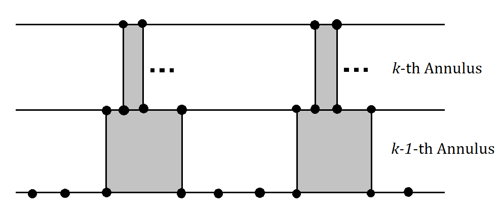
For the first statement, it is easy to construct the Hamiltonian cycle in , in a recursive manner. We start by a planar annular projection of . We include the interior face in the interior of a path connected region . Recalling our convention that, the -face-only partition in the outer annulus of an ADB-AC graph is assumed to be , we can describe this strategy by extending through -th annulus by coloring the faces in in grey, for every -recursively. Thus we gradually extend following the strategy shown in Figure 5. It is easy to see that, when we recursively apply this strategy for all the annuli in , the boundary of the final path connected region would manifest into a Hamiltonian cycle. We will call this strategy of constructing Hamiltonian cycles henceforth as the pyramid strategy.
Recall that, as per our convention, the -face-only partition in the outer annulus of an ADB-AC graph is assumed to be . Let . For the second statement, note that for any , , if the edges interior to -th annulus in are attached to faces that are not in -cycle-only face partition in , , where is the annular restriction of , then for the -th annulus, there is a -cycle. The reason is no edges in the -th annulus are attached to the face partition with -cycles of the -th annulus. Thus by Lemma 3.2, has to be Hamiltonian. The Hamiltonian cycle can be constructed using the same strategy as depicted in Figure 3.2. We will call this strategy of constructing Hamiltonian cycles henceforth as the ring strategy. ∎
Let be ADB-AC graph drawn on a plane. From Theorem 3.7, it is evident that the annuli of can be one of two possible types depending on how the edges in the interior of a given annulus are attached to the previous annulus. For the -th annulus , in if the edges in the interior of the annulus are attached to the -th annulus such that the edges are attached to the faces in the face partition of consisting of only -cycles, then we call a block annulus, otherwise we call a ring annulus. We can thus restate Theorem 3.7 as: Given an ADB-AC graph , if consists of only block annuli or only ring annuli, then is Hamiltonian. Note that the spider-web graphs that motivated the work are a subclass of ADB graphs that consist of only block annuli. Also note that given a planar representation ADB-AC graph , the first and second annulus can be considered both a block annulus and a ring annulus. By convention, we will consider them as of the same category as the third annulus.
Corollary 3.8.
Let be an ADB-AC graph consisting only of ring annuli, . Let denote the number of faces in an annulus. Then must have at least Hamiltonian cycles.
Proof.
Let be an ADB-AC graph consisting only of ring annuli . Any arbitrary annulus must have -cycles. One -cycle from every annuli can be used to create a Hamiltonian cycle. Thus, it is clear that has at least Hamiltonian cycles. Given that is at least , we can derive that any such graph will have at least Hamiltonian cycles. ∎
In Theorem 3.7, we have already discussed a strategy of finding Hamiltonian cycles in an ADB-AC graph , given that consists of only block annuli. Now we will explore some more strategies to find a Hamiltonian cycle in .
Lemma 3.9.
Let us consider an ADB-AC graph , with annuli, containing only block annuli. There are at least two more strategies for finding Hamiltonian cycles in , in addition to the one described in Theorem 3.7.
Proof.
Recall that, as per our convention, the -face-only partition in the outer annulus of an ADB-AC graph is assumed to be . Let . Let us consider a planar projection of such that and are fixed and well defined. Note that such a graph must contain a specific substructure described as follows. This substructure contains one face from every annulus such that the faces are stacked on each other ( faces stacked on one another). Let us denote these faces as and observe that for the annular restriction of , . Also the face in the -th annulus is a -cycle. Existence of such a structure is ensured due to the fact that has only block annuli. We call such a structure a pyramid. Now, note that, since is -edge connected, there has to be at least two pyramids in . We denote them as and .
Note that, in the first annulus of , there must exist a partition of faces with all -cycles. We choose one from them and call it . Our strategy to build a second Hamiltonian cycle in is based on these pyramids and the -cycle . The strategy is as follows:
- 1.
-
2.
Note that all the faces in and are colored in grey, i.e. are interior to the cycle. Also, is colored in white, i.e. is exterior to the cycle.
-
3.
Remove from , i.e color in white.
-
4.
Color all faces in annulus except for . Call the new grey region .
-
5.
Remove coloring from all faces in annulus except for the face in annulus that belongs in .
-
6.
Color all faces in annulus except for the -cycles attached to the face , such that and any one -cycle attached to the face , such that . Also, we choose such that the .
-
7.
Among the uncolored -cycles mentioned in the step above, color the ones that are in .
After Step , the grey region gets path-disconnected but retains path-connectivity after Step . Step also gives a Hamiltonian cycle in . After Step , note that only some vertices in the outer boundary of the -th annulus are in the interior of the white region. After Step these vertices again lie in the boundary of the grey-white region. Note both the grey and white regions still remain path connected (the existence of ensures the path connectedness of the white region). After Step all the vertices lie in the boundary of the grey-white coloring and both the white and the grey region remain path connected. Thus the boundary of the grey-white path connected regions is a new Hamiltonian cycle . We will call this strategy of constructing a Hamiltonian cycle in as pyramid-ring strategy or pr-strategy. The pr-strategy have been demonstrated in Figure 6. ∎
Theorem 3.10.
Let us consider a planar annular-embedding of an ADB-AC graph , with annuli, containing a sequence of block annuli followed by a sequence of ring annuli. Then is Hamiltonian.
Proof.
Recall that, as per our convention, the -face-only partition in the outer annulus of an ADB-AC graph is termed as . When we treat all the annuli as ring annuli. For block annuli, we first employ the pr-strategy on . Since the -th annulus and all annuli afterwards are ring annuli, there must exist a -cycle in the -th annulus such that the edges of the face are attached to some face . Since all the faces in are marked in grey as per the pr-strategy, we can extend the grey color to and follow the ring strategy for the rest of the annuli after that to obtain a Hamiltonian cycle (whose interior is marked in grey). ∎
Theorem 3.11.
Let us consider a planar annular embedding of an ADB-AC graph , with annuli, containing a sequence of ring annuli followed by a sequence of block annuli. Then is Hamiltonian.
Proof.
If , then we can consider all the annuli as block annuli and use the pr-strategy for finding a Hamiltonian cycle. Recall that, as per our convention, the -face-only partition in the outer annulus of an ADB-AC graph is termed as . If , first we can create a Hamiltonian cycle in using the ring strategy, and color it’s interior grey such that only one -face in is colored in white. Until now, for -th annulus in , the -face-only face partition has been conventionally . We alter this convention from this annulus and call them . Note that, this allows us to extend the grey region (Hamiltonian cycle) from th annulus to the th annulus, using the pr-strategy as described in Lemma 3.9. ∎
Theorem 3.12.
Every ADB-AC graph , with arbitrary sequence of ring and block annuli is Hamiltonian, if every sequence ring annuli that lies between two sequences of block annuli, has length at least , that is, there are only non singular sequences of ring annuli in .
Open questions
We propose the following open questions from our study:
-
1.
Are all ADB-AC graphs Hamiltonian?
-
2.
Are all ADB graphs Hamiltonian?
Acknowledgements
I thank my PhD supervisor Olaf Wolkenhauer for his constant encouragement and unfaltering support for this research. This work was in part supported by funds from Bioinformatics Infrastructure (de.NBI) and Establishment of Systems Medicine Consortium in Germany e:Med , as well as the German Federal Ministry for Education and Research (BMBF) programs (FKZ 01ZX1709C). I thank Miss Shukla Sarkar for her patient support.
References
- [1] Behrooz Bagheri Gh, Tomas Feder, Herbert Fleischner, and Carlos Subi. Hamiltonian cycles in planar cubic graphs with facial 2-factors, and a new partial solution of barnette’s conjecture. Journal of Graph Theory, pages 1–20, 2020.
- [2] Jean-Claude Bermonf, Johny Bond, Carole Martin, Aleksandar Pekec, and Fred S. Roberts. Optimal orientations of annular networks. Journal of Interconnection Networks, 01(01):21–46, 2000.
- [3] Jan Florek. On barnette’s conjecture. Discrete Mathematics, 310(10):1531 – 1535, 2010.
- [4] Jan Florek. On barnette’s conjecture and h+-h+- property. Electron. Notes Discret. Math., 43:375–377, 2013.
- [5] Jan Florek. Remarks on barnette’s conjecture. Journal of Combinatorial Optimization, 39(1):149 – 155, 2020.
- [6] M. Hasheminezhad, S. Mehdi Hashemi, B. McKay, and M. Tahmasbi. Rectangular-radial drawings of cubic plane graphs. Computational Geometry, 43(9):767 – 780, 2010.
- [7] D. A. Holton, B. Manvel, and B. D. McKay. Hamiltonian cycles in cubic -connected bipartite planar graphs. J. Combin. Theory Ser. B, 38(3):279–297, 1985.
- [8] D.A Holton and B.D McKay. The smallest non-hamiltonian 3-connected cubic planar graphs have 38 vertices. Journal of Combinatorial Theory, Series B, 45(3):305 – 319, 1988.
- [9] J.D. Horton. On two-factors of bipartite regular graphs. Discrete Mathematics, 41(1):35 – 41, 1982.
- [10] Shin-Shin Kao and Lih-Hsing Hsu. Spider web networks: a family of optimal, fault tolerant, hamiltonian bipartite graphs. Applied Mathematics and Computation, 160(1):269 – 282, 2005.
- [11] Xiaoyun Lu. A note on barnette’s conjecture. Discrete Mathematics, 311(23):2711 – 2715, 2011.
- [12] Grace Misereh and Yuri Nikolayevsky. Annular and pants thrackles. Discret. Math. Theor. Comput. Sci., 20, 2018.
- [13] W. T. Tutte. On Hamiltonian circuits. J. London Math. Soc., 21:98–101, 1946.