Hard-Negative Sampling for Contrastive Learning: Optimal Representation Geometry and Neural- vs Dimensional-Collapse
Abstract
For a widely-studied data model and general loss and sample-hardening functions we prove that the losses of Supervised Contrastive Learning (SCL), Hard-SCL (HSCL), and Unsupervised Contrastive Learning (UCL) are minimized by representations that exhibit Neural-Collapse (NC), i.e., the class means form an Equiangular Tight Frame (ETF) and data from the same class are mapped to the same representation. We also prove that for any representation mapping, the HSCL and Hard-UCL (HUCL) losses are lower bounded by the corresponding SCL and UCL losses. In contrast to existing literature, our theoretical results for SCL do not require class-conditional independence of augmented views and work for a general loss function class that includes the widely used InfoNCE loss function. Moreover, our proofs are simpler, compact, and transparent. Similar to existing literature, our theoretical claims also hold for the practical scenario where batching is used for optimization. We empirically demonstrate, for the first time, that Adam optimization (with batching) of HSCL and HUCL losses with random initialization and suitable hardness levels can indeed converge to the NC-geometry if we incorporate unit-ball or unit-sphere feature normalization. Without incorporating hard-negatives or feature normalization, however, the representations learned via Adam suffer from Dimensional-Collapse (DC) and fail to attain the NC-geometry. These results exemplify the role of hard-negative sampling in contrastive representation learning and we conclude with several open theoretical problems for future work. The code can be found at https://github.com/rjiang03/HCL/tree/main
Keywords: Contrastive Learning, Hard-Negative Sampling, Neural-Collapse.
1 Introduction
Contrastive representation learning (CL) methods learn a mapping that embeds data into a Euclidean space such that similar examples retain close proximity to each other and dissimilar examples are pushed apart. CL, and in particular unsupervised CL, has gained prominence in the last decade with notable success in Natural Language Processing (NLP), Computer Vision (CV), time-series, and other applications. Recent surveys [2, 23] and the references therein provide a comprehensive view of these applications.
The characteristics and utility of the learned representation depend on the joint distribution of similar (positive samples) and dissimilar data points (negative samples) and the downstream learning task. In this paper we are not interested in the downstream analysis, but in characterizing the geometric structure and other properties of global minima of the contrastive learning loss under a general latent data model. In this context, we focus on understanding the impact and utility of hard-negative sampling in the UCL and SCL settings. When carefully designed, hard-negative sampling improves downstream classification performance of representations learned via CL as demonstrated in [24], [11, 10], and [17]. While it is known that hard-negative sampling can be performed implicitly by adjusting what is referred to as the temperature parameter in the CL loss, in this paper we set this parameter to unity and explicitly model hard-negative sampling through a general “hardening” function that can tilt the sampling distribution to generate negative samples that are more similar to (and therefore harder to distinguish from) the positive and anchor samples. We also numerically study the impact of feature normalization on the learned representation geometry.
1.1 Main contributions
Our main theoretical contributions are Theorems 1, 2, and 3, which, under a widely-studied latent data model, hold for any convex, argument-wise non-decreasing contrastive loss function, any non-negative and argument-wise non-decreasing hardening function to generate hard-negative samples, and norm-bounded representations of dimension at least .
Theorem 1 establishes that the HSCL loss dominates the SCL loss and similarly the HUCL loss dominates the UCL loss. In this context we note that Theorem 3.1 in [30] is a somewhat similar result for the UCL setting, but for a special loss function and it does not address directly hard-negatives.
Theorem 2 is a novel result which states that the globally optimal representation geometry for both SCL and HSCL corresponds to Neural-Collapse (NC) (see Definition 6) with the same optimal loss value. In contrast to existing works (see related works section 2), we show that achieving NC in SCL and HSCL does not require class-conditional independence of the positive samples.
Similarly, Theorem 3 establishes the optimality of NC-geometry for UCL if the representation dimension is sufficiently large compared to the number of latent classes which, in turn, is implicitly determined by the joint distribution of the positive examples that corresponds to the augmentation mechanism.
A comprehensive set of experimental results on one synthetic and three real datasets are detailed in Sec. 5 and Appendix B. These include experiments that study effects of two initialization methods, three different feature normalization methods, three different batch sizes, two very different families of hardening functions, and two different CL sampling strategies. Empirical results show that when using the Adam optimizer with random initialization, the matrix of class means for SCL is badly conditioned and effectively low-rank, i.e., it exhibits Dimensional-Collapse (DC). In contrast, the use of hard-negatives at appropriate hardness levels mitigates DC and enables convergence to the global optima. A similar phenomenon is observed in the unsupervised settings. We also show that feature normalization is critical for mitigating DC in these settings. Results are qualitatively similar across different datasets, a range of batch sizes, hardening functions, and CL sampling strategies.
2 Related work
2.1 Supervised Contrastive Learning
The theoretical results for our SCL setting, where in contrast to [7] and [13] we make use of label information in positive as well as negative sampling, are novel. The debiased SCL loss in [5] corresponds to our SCL loss, but no analysis pertaining to optimal representation geometry was considered in [5]. A recent ArXiv preprint by [6], which appeared after our own ArXiv preprint, [11], considers using label information for negative sampling in SCL with InfoNCE loss, calling it the SINCERE loss. Our theoretical results prove that NC is the optimal geometry for the SINCERE loss. Furthermore, our results and analysis also apply to hard-negative sampling as well, a scenario not considered thus far for SCL.
We would like to note that our theoretical set-up for UCL under the sampling mechanism of Figure 1, can be seen to be aligned with the SCL analysis that makes use of label information only for positive samples as done in [13] and [7]. Therefore, our theoretical results provide an alternative proof of optimality of NC based on simple, compact, and transparent probabilistic arguments complementing the proof of a similar result in [7]. We note that similarly to [7], our arguments also hold for the case when one approximates the loss using batches.
We want to point out that in all key papers that conduct a theoretical analysis of contrastive learning e.g., [1, 7, 25], the positive samples are assumed to be conditionally i.i.d., conditioned on the label. However, this conditional independence may not hold in practice when using augmentation mechanisms typically considered in CL settings e.g., [19, 20, 31, 4].
Unlike the recent work of [33] which shows that the optimization landscape of supervised learning with least-squares loss is benign, i.e. all critical points other than the global optima are strict saddle points, in Sec. 5 we demonstrate that the optimization landscape of SCL is more complicated. Specifically, not only may the global optima not be reached by SGD-like methods with random initialization, but also the local optima exhibit the Dimensional-Collapse (DC) phenomenon. However, our experiments demonstrate that these issues are remedied via HSCL whose global optimization landscape may be better. Here we note that [32] show that with unit-sphere normalization, Riemannian gradient descent methods can achieve the global optima for SCL, underscoring the importance of optimization methods and constraints for training in CL.
2.2 Unsupervised Contrastive Learning
[27] argue that asymptotically (in number of negative samples) the InfoNCE loss for UCL optimizes for a trade-off between the alignment of positive pairs while ensuring uniformity of features on the hypersphere. However, a non-asymptotic and global analysis of the optimal solution is still lacking. In contrast, for UCL in Theorem 3, we show that as long as the embedding dimension is larger than the number of latent classes, which in turn is determined by the distribution of the similar samples, the optimal representations in UCL exhibit NC-geometry.
Our results also complement several recent papers, e.g., [22], [29], [28], that study the role of augmentations in UCL. Similar to theoretical works analyzing UCL, e.g. [1] and [16], our results also assume conditional independence of positive pairs given the label. This assumption may or may not be satisfied in practice.
We demonstrate that a recent result, viz., Theorem 4 in [12], that attempts to explain DC in UCL is limited in that under a suitable initialization, the UCL loss trained with Adam does not exhibit DC (see Sec. 5). Furthermore, we demonstrate empirically, for the first time, that HUCL mitigates DC in UCL at moderate hardness levels. For CL (without hard-negative sampling), [34] characterize local solutions that correspond to DC but leave open the analysis of training dynamics leading to collapsed solutions.
A geometrical analysis of HUCL is carried out in [24], but the optimal solutions are only characterized asymptotically (in the number of negative samples) and for the case when hardness also goes to infinity, the analysis seems to require knowledge of supports of class conditional distributions. In contrast, we show that the geometry of the optimal solution for HUCL depends on the hardness level and is, in general, different compared to UCL due to the possibility of class collision.
3 Contrastive Learning framework
3.1 Mathematical model
Notation: . For , , , and . If , and are “null”.
Let denote a (deterministic) representation mapping from data space to representation space . Let denote a family of such representation mappings. Contrastive Learning (CL) selects a representation from the family by minimizing an expected loss function that penalizes “misalignment” between the representation of an anchor sample and the representation of a positive sample and simultaneously penalizes “alignment” between and the representations of negative samples .
We consider a CL loss function of the following general form.
Definition 1 (Generalized Contrastive Loss).
| (1) |
where is a convex function that is also argument-wise non-decreasing (i.e., non-decreasing with respect to each argument when the other arguments are held fixed) throughout .
This subsumes and generalizes popular CL loss functions such as InfoNCE and triplet-loss with sphere-normalized representations. InfoNCE corresponds to with 111This is the log-sum-exponential function which is convex over for all and strictly convex over if . and , , is the triplet-loss with sphere-normalized representations. However, some CL losses such as the spectral contrastive loss of [8] are not of this form.
The CL loss is the expected value of the CL loss function:
where is the joint probability distribution of the anchor, positive, and negative samples and is designed differently within the supervised and unsupervised settings as described below.
Supervised CL (SCL): Here, all samples have class labels: a common class label for the anchor and positive sample and one class label for each negative sample denoted by for the -th negative sample, . The joint distribution of all samples and their labels is described in the following equation:
| (2) | ||||
| (3) |
where for all is the marginal distribution of the anchor’s label and is the conditional probability distribution of any negative sample given its class .
This joint distribution may be interpreted from a sample generation perspective as follows: first, a common class label for the anchor and positive sample is sampled from a class marginal probability distribution . Then, the anchor and positive samples are generated by sampling from the conditional distribution . Then, given and their common class label , the negative samples and their labels are generated in a conditionally IID manner. The sampling of , for each , can be interpreted as first sampling a class label different from in a manner consistent with the class marginal probability distribution (sampling from distribution ) and then sampling from the conditional probability distribution of negative samples given class . Thus in SCL, the negative samples are conditionally IID and independent of the anchor and positive sample given the anchor’s label.
In the typical supervised setting, the anchor, positive, and negative samples all share the same common conditional probability distribution within each class given their respective labels.
We denote the CL loss in the supervised setting by .
Unsupervised CL (UCL): Here samples do not have labels or rather they are latent (unobserved) and the negative samples are IID and independent of the anchor and positive samples.
Latent labels in UCL can be interpreted as indexing latent clusters. Suppose that there are latent clusters from which the anchor, positive, and the negative samples can be drawn from. Then the joint distribution of all samples and their latent labels can be described by the following equation:
| (4) |
where is the marginal distribution of the anchor’s latent label, the marginal distribution of the latent labels of negative samples, and is the conditional probability distribution of any negative sample given its latent label . We have used the same notation as in SCL (and slightly abused it for ) in order to make the similarities and differences between the SCL and UCL distribution structures transparent.
In the typical UCL setting, and the conditional distribution of given its label and the conditional distribution of given its label are both which is the conditional distribution of any negative sample given its label.
We denote the CL loss in the unsupervised setting by .
Anchor and positive samples: For the SCL scenario, we will consider sampling mechanisms in which the representations of the anchor and the positive sample have the same conditional probability distribution given their common label (see (2)). We will not, however, assume that and are conditionally independent given . This is compatible with settings where and are generated via IID augmentations of a common reference sample as in SimCLR [4] (see Fig. 1 for the model and Appendix A for a proof of compatibility of this model).
For UCL, we assume the same mechanism for sampling the positive samples as that for SCL, but the latent label is unobserved. Further, the negative samples are generated independently of the positive pairs using the same mechanism, e.g., IID augmentations of an chosen independently of (see Fig. 1). Thus, the anchor, positive, and negative samples will all have the same marginal distribution given by .
3.2 Hard-negative sampling
Hard-negative sampling aims to generate negative samples whose representations are “more aligned” with that of the anchor (making them harder to distinguish from the anchor) compared to a given reference negative sampling distribution (whether unsupervised or supervised). We consider a very general class of “hardening” mechanisms that include several classical approaches as special cases. To this end, we define a hardening function as follows.
Definition 2 (Hardening function).
is a hardening function if it is non-negative and argument-wise non-decreasing throughout .
Hard-negative SCL (HSCL): From (2) it follows that in SCL, is the reference negative sampling distribution for one negative sample and is the reference negative sampling distribution for negative samples. Let be a hardening function such that for all and all ,
Then we define the -harder negative sampling distribution for SCL as follows.
Definition 3 (-harder negatives for SCL).
| (5) |
Observe that negative samples which are more aligned with the anchor in the representation space, i.e., is large, are sampled relatively more often in than in the reference because is argument-wise non-decreasing throughout .
In HSCL, are conditionally independent of given and but they are not conditionally independent of given (unlike in SCL). Moreover, may not be conditionally IID given if the hardening function is not (multiplicatively) separable. We also note that unlike in SCL, depends on the representation function .
We denote the joint probability distribution of all samples and their labels in the hard-negative SCL setting by and the corresponding CL loss by .
Hard-negative UCL (HUCL): From (4) it follows that in UCL, is the reference negative sampling distribution for one negative sample and is the reference negative sampling distribution for negative samples. Let be a hardening function such that for all ,
| (6) |
Then we define the -harder negative sampling probability distribution for UCL as follows.
Definition 4 (-harder negatives for UCL).
| (7) |
Again, observe that negative samples which are more aligned with the anchor in representation space, i.e., is large, are sampled relatively more often in than in the reference because is argument-wise non-decreasing throughout .
In HUCL, are conditionally independent of given , but they are not independent of (unlike in UCL). Moreover, may not be conditionally IID given if the hardening function is not (multiplicatively) separable. We also note that unlike in UCL, depends on the representation function .
We denote the joint probability distribution of all samples and their (latent labels) in the hard-negative UCL setting by and the corresponding CL loss by .
4 Theoretical results
In this section, we present all our theoretical results using the notation and mathematical framework for CL described in the previous section.
4.1 Hard-negative CL loss is not smaller than CL loss
Theorem 1 (Hard-negative CL versus CL losses).
Let in (1) be argument-wise non-decreasing over and assume that all expectations associated with , , , exist and are finite. Then, for all and all , and .
We note that convexity of is not needed in Theorem 1. The proof of Theorem 1 is based on the generalized (multivariate) association inequality due to Harris, Theorem 2.15 [3] and its corollary which are stated below.
Lemma 1 (Harris-inequality, Theorem 2.15 in [3]).
Let and be argument-wise non-decreasing throughout . If then
whenever the expectations exist and are finite.
Corollary 1.
Let be non-negative and argument-wise non-decreasing throughout such that . Let . If is argument-wise non-decreasing throughout such that exists and is finite, then
Proof of Theorem 1. The proof essentially follows from Corollary 1 by defining for , defining , noting that are conditionally IID given in the UCL setting and conditionally IID given in the SCL setting, and verifying that the conditions of Corollary 1 hold.
For clarity, we provide a detailed proof of the inequality . The detailed proof of the inequality parallels that for the (more intricate) supervised setting and is omitted.
4.2 Lower bound for SCL loss and Neural-Collapse
Consider the SCL model with anchor, positive, and negative samples generated as described in Sec. 3.1. Within this setting, we have the following lower bound for the SCL loss and conditions for equality.
Theorem 2 (Lower bound for SCL loss and conditions for equality with unit-ball representations and equiprobable classes).
In the SCL model with anchor, positive, and negative samples generated as described in (2) and (3), let (a) for all (equiprobable classes), (b) (unit-ball representations), and (c) the anchor, positive and negative samples have a common conditional probability distribution within each class given their respective labels. If is a convex function that is also argument-wise non-decreasing throughout , then for all ,
| (11) |
For a given and all , let
| (12) |
If a given satisfies the following additional condition:
| (13) |
then equality will hold in (11), i.e., additional condition (13) is sufficient for equality in (11). Additional condition (13) also implies the following properties:
-
(i)
zero-sum class means: ,
-
(ii)
unit-norm class means: ,
-
(iii)
.
-
(iv)
zero within-class variance: for all and all , , and
-
(v)
The support sets of for all must be disjoint and the anchor, positive and negative samples must share a common deterministic labeling function defined by the support sets.
-
(vi)
equality of HSCL and SCL losses:
If is a strictly convex function that is also argument-wise strictly increasing throughout , then additional condition (13) is also necessary for equality to hold in (11).
Proof We have
| (14) | |||
| (15) | |||
| (16) | |||
| (17) | |||
| (18) | |||
| (19) | |||
| (20) |
which is the lower bound in (11). Inequality (14) is because is argument-wise non-decreasing and by the Cauchy-Schwartz inequality since (unit-ball representations). Inequality (15) is Jensen’s inequality applied to the convex function . Equality (16) is due to the law of iterated expectations. Equality (17) follows from (2), (3), and the assumption of equiprobable classes. Equality (18) is because . Inequality (19) is because is argument-wise non-decreasing and the smallest possible value of is zero and the largest possible value of is one (unit-ball representations): Jensen’s inequality for the strictly convex function together with (unit-ball representations) imply that for all , we have
| (21) |
Finally the equality (20) is because .
and Proof that additional condition (13) implies zero-sum and unit-norm class means: Inequality (21) together with condition (13) implies that
Thus and for all , .
Let . Then from (13) and , the gram matrix where is the identity matrix and is the column vector of all ones. From this it follows that has one eigenvalue of zero corresponding to eigenvector and eigenvalues all equal to corresponding to orthogonal eigenvectors spanning the orthogonal complement of . Thus, has nonzero singular values all equal to and a rank equal to .
Proof that additional condition (13) implies zero within-class variance: We just proved that additional condition (13) together with the unit-ball representation constraint implies unit-norm class means. This, together with (21) implies that for all ,
| (22) |
This implies that we have equality in Jensen’s inequality, which can occur iff with probability one given , we have (since is strictly convex). Since the anchor, positive and negative samples all have a common conditional probability distribution within each class given their respective labels, it follows that for all and all , . Moreover, since the anchor and positive samples have the same label, for all , with probability one given , we have .
Proof that additional condition (13) is sufficient for equality to hold in (11): From the proofs of , and above, if additional condition (13) holds, then we showed that with probability one given we have (see the para below (22)). This equality of and is a conditional equality given the class. Since this is true for all classes, it implies equality (with probability one) of and without conditioning on the class:
| (23) |
From (23) we get
| (24) |
since with probability one given and . Equality in (14) then follows from (23) and (24). Moreover, due to zero within-class variance we will have
| (25) |
and then we will have equality in (15) and (19). Therefore additional condition (13) is a sufficient condition for equality to hold in (11).
Proof that support sets of are disjoint: From part , all samples belonging to the support set of , are mapped to by . From part and condition (13), distinct labels have distinct representation means: for all , if , then . Therefore the support sets of for all must be disjoint. Since the anchor, positive, and negative samples all share a common conditional probability distribution and the same marginal label distribution , it follows that they share a common conditional distribution of label given sample (labeling function). Since the support sets of for all are disjoint, the labeling function is deterministic and is defined by the support set to which a sample belongs.
Proof of equality of HSCL and SCL losses under additional condition (13): under the equal inner-product class means condition, with probability one simultaneously for all and , a constant. Consequently, for all and the given , we must have which would imply that (see Equation 5) and therefore where the last equality is because additional condition (13) is sufficient for equality to hold in (11).
Proof that additional condition (13) is necessary for equality in (11) if is strictly convex and argument-wise strictly increasing over : If equality holds in (11), then it must also hold in (14), (15), and (19). If is argument-wise strictly increasing, then equality in (19) can only occur if all class means have unit norms. Then, from (22) and the reasoning in the paragraph below it, we would have zero within-class variance and equations (23) and (24). This would imply equality in (14). If is strictly convex then equality in (15), which is Jensen’s inequality, can only occur if for all , for some constants . Since has the same distribution for all , it follows that for all , for some constant . Since we have already proved zero within-class variance and the labels of negative samples are always distinct from that of the anchor, it follows that for all , we must have . Since we have equality in (14) and is argument-wise strictly increasing, we must have which implies that additional condition (13) must hold (it is a necessary condition).
Remark 1.
We note that Theorem 2 also holds if we have unit-sphere representations (a stronger constraint) as opposed to unit-ball representations, i.e., if : the lower bound (11) holds since the unit sphere is a subset of the unit ball and equality can be attained with unit-sphere representations in Theorem 2.
Remark 2.
Definition 5 (ETF).
Definition 6 (CL Neural-Collapse (NC)).
Remark 3.
The term “Neural-Collapse” was originally used for representation mappings implemented by deep classifier neural networks (see [21]). However, here we use the term more broadly for any family of representation mappings and within the context of CL instead of classifier training.
The following corollary is a partial restatement of Theorem 2 in terms of CL Neural-Collapse:
Corollary 2.
Under the conditions of Theorem 2, equality in (11) is attained by any representation map that exhibits CL Neural-Collapse. Moreover, if is strictly convex and argument-wise strictly increasing over , then equality in (11) is attained by a representation map , if, and only if, it exhibits CL Neural-Collapse.
4.3 Empirical and batched empirical SCL losses
Empirical SCL loss: Theorem 2 also holds for empirical SCL loss because simple averages over samples can be expressed as expectations with suitable uniform distributions over the samples. If the family of representation mappings has sufficiently high capacity (e.g., the family of mappings implemented by a sufficiently deep and wide feed-forward neural network) and , is a discrete probability mass function (pmf) over a finite set (e.g., uniform pmf over training samples within each class) with support-sets that are disjoint across different classes, then the equal inner-product condition (13) in Theorem 2 can be satisfied for a suitable in the family. If either convexity or monotonicity of is not strict, e.g., , then it may be possible for a representation map to attain the lower bound without exhibiting CL Neural-Collapse.
Batched empirical SCL loss: We will now show that representations that exhibit CL Neural-Collapse will also minimize batched empirical SCL loss under the conditions of Theorem 2. Here, the full data set has balanced classes (equal number of samples in each class) but is partitioned into disjoint nonempty batches of possibly unequal size. Let denote the batch index and the number of samples in batch . Let denote the empirical SCL loss in batch and
the overall batched empirical SCL loss. Note that in a given batch the data may not be balanced across classes and therefore we cannot simply use Theorem 2, which assumes balanced classes, to deduce the optimality of CL Neural-Collapse representations.
We lower bound the batched empirical SCL loss as follows:
| (26) | ||||
| (27) | ||||
| (28) | ||||
| (29) |
where inequality (26) holds for the same reason as in (14), inequality (27) is Jensen’s inequality applied to which is convex, and equality (28) is due to the law of iterated (empirical) expectation. The right side of (27) is precisely the right side of (15) and therefore (29) follows from (15) – (20). From the above analysis it follows that the arguments used to prove Theorem 2 can be applied again to prove that the conclusions of Theorem 2 and Corollary 2 also hold for the batched empirical SCL loss.
4.4 Lower bound for UCL loss with latent labels and Neural-Collapse
Consider the UCL model with anchor, positive, and negative samples generated as described in Sec. 3.1. Within this setting, we have the following lower bound for the UCL loss and conditions for equality.
Theorem 3 (Lower bound for UCL loss with latent labels and conditions for equality with unit-ball representations and equiprobable classes).
In the UCL model with anchor, positive, and negative samples generated as described in (4), let (a) for all (equiprobable classes), (b) (unit-ball representations), (c) the anchor, positive and negative samples have a common conditional probability distribution within each latent class given their respective labels, (d) in (4), and (e) the anchor and positive samples are conditionally independent given their common label, i.e., in (4).222As discussed in Sec. 2, all existing works that conduct a theoretical analysis of UCL make this assumption. If is a convex function that is also argument-wise non-decreasing throughout , then for all ,
| (30) |
where is the indicator function. For a given and all , let be as defined in (12). If a given satisfies additional condition (13), then equality will hold in (30), i.e., additional condition (13) is sufficient for equality in (30). Additional condition (13) also implies the following properties:
-
(i)
zero-sum class means: ,
-
(ii)
unit-norm class means: ,
-
(iii)
.
-
(iv)
zero within-class variance: for all and all , , and
-
(v)
The support sets of for all must be disjoint and the anchor, positive and negative samples must share a common deterministic (latent) labeling function defined by the support sets.
If is a strictly convex function that is also argument-wise strictly increasing throughout , then additional condition (13) is also necessary for equality to hold in (30).
Proof For , we define the following indicator random variables and note that for all , is a deterministic function of . Since and , it follows that and independent of . We then have the following sequence of inequalities:
| (31) | |||
| (32) | |||
| (33) | |||
| (34) | |||
| (35) | |||
| (36) | |||
| (37) | |||
| (38) | |||
| (39) | |||
| (40) | |||
| (41) |
where the validity of each numbered step in the above sequence of inequalities is explained below.
Inequality (31) is Jensen’s inequality conditioned on applied to the convex function . Equality (32) holds because for every , we have and are conditionally independent given and (per the UCL model (4)), and are conditionally independent given their common label (assumption (d) in the theorem statement), and the class means in representation space are as defined in (12). Inequality (33) is Jensen’s inequality conditioned on applied to the convex function . Equality (34) holds because for all , . Equality (35) holds because only takes values , and if , then and . Therefore the expressions to the right of the equality symbols in (34) and (35) match when and when . Inequality (36) is because is non-decreasing and for all because all representations are in the unit closed ball. Equality (37) holds because for each , and when . Equality (38) follows from elementary linear algebraic operations. Inequality (39) holds because is argument-wise non-decreasing, the smallest possible value for is zero and the largest possible value for , for all , is one. Equality (41) follows from the definition of the indicator variables in terms of and because are IID .
Similarly to the proof of Theorem 2, if additional condition (13) holds for some , then properties – in Theorem 3 hold. Moreover, then (23), (24), and (25) also hold and then we will have equality in (31), (33), (36) and (39). Thus additional condition (13) is sufficient for equality to hold in (30).
Proof that additional condition (13) is necessary for equality in (30) if is strictly convex and argument-wise strictly increasing over : If equality holds in (30), then it must also hold in (31), (33), (36), and (39). If is argument-wise strictly increasing, then equality in (39) can only occur if all class means have unit norms (which would also imply equality in (36)). Then, from (22) and the reasoning in the paragraph below it, we would have zero within-class variance and (24), which would imply that with probability one for all , and which would imply equality in (31) as well. Equality in (33) together with strict convexity of and would imply that with probability one, for all , given we must have some deterministic function of and if is also argument-wise strictly increasing, then this function must be such that due to (40). This would imply that for all , we must have .
Thus for all , i.e., (and this has nonzero probability), which is the additional condition (13). Thus the additional condition (13) must hold (it is a necessary condition).
Counterparts of Corollary 2 and results for empirical SCL loss and batched empirical SCL loss can be stated and derived for UCL. One important difference between results for SCL and UCL is that Theorem 3 is missing the counterpart of property in Theorem 2. Unlike in Theorem 2, we cannot assert that if the lower bound is attained, then we will have . This is because in the UCL and HUCL settings, the negative sample can come from the same latent class as the anchor (latent class collision) with a positive probability (). Then for a representation that exhibits Neural-Collapse, we cannot conclude that with probability one we must have , for some constant . Deriving a tight lower bound for HUCL and determining whether it can be attained iff there is Neural-Collapse in UCL (under suitable conditions), are open problems.
Neural-Collapse in SCL or UCL requires that the representation space dimension (see part of Theorems 2 and 3). This can be ensured in practical implementations of SCL since labels are available and the number of classes is known. In UCL, however, not just latent labels, but even the number of latent classes is unknown. Thus even if it was possible to attain the global minimum of the empirical UCL loss with an exhibiting Neural-Collapse, we may not observe Neural-Collapse with an argument-wise strictly increasing and strictly convex unless is chosen to be sufficiently large.
In practice, even without knowledge of latent labels, it is possible to design a sampling distribution having a structure that is compatible with (4) and conditions (c) and (d) of Theorem 3, e.g, via IID augmentations of a reference sample as in SimCLR illustrated in Fig. 1. However, it is impossible to ensure that the equiprobable latent class condition (a) or the anchor-positive conditional independence condition (d) in Theorem 3 hold or that the supports of determined by the sample augmentation mechanism will be disjoint across all latent classes. Thus a representation minimizing UCL loss may not exhibit Neural-Collapse even if is strictly convex and argument-wise strictly increasing or it might exhibit zero within-class variance, but the class means may not form an ETF (see [26]).
A second important difference between theoretical results for SCL and UCL is that unlike in Theorem 2, conditional independence of the anchor and positive samples given their common label is assumed in Theorem 3 (condition (d) in the theorem). It is unclear whether the results of Theorem 3 for the UCL setting will continue to hold in entirety without conditional independence and we leave this as an open problem.
5 Practical achievability of global optima
We first verify our theoretical results using synthetic data comprising three classes with 100 data points per class. The points within each class are IID with a 3072-dimensional Gaussian distribution having an identity covariance matrix and a randomly generated mean vector having IID components that are uniformly distributed over . We explored two strategies for constructing anchor-positive pairs:
-
•
Using Label Information: For each anchor sample, a positive sample is chosen uniformly from among all samples having the same label as the anchor (including the anchor). all samples that share the same label with the anchor are used to form the positive pairs. Note that the anchor and the positive can be identical.
-
•
Additive Gaussian Noise Augmentation Mechanism: For each (reference) sample, we generate the anchor sample by adding IID zero-mean Gaussian noise of variance to all dimensions of the reference sample. The corresponding positive sample is generated in the same way from the reference sample using noise that is independent of that used to generate the anchor.
The data dimension of 3072 allows for reshaping the vector into a tensor which can be processed by ResNet. We then investigate the achievability of global-optima for UCL, SCL, HUCL, and HSCL on the following three real-world image datasets: CIFAR10, CIFAR100 [14], and TinyImageNet [15]. These datasets consist of images across 10 classes (CIFAR10), 100 classes (CIFAR100), and 200 classes (TinyImageNet), respectively. Similar phenomena are observed in all three datasets. We present results for CIFAR100 here and results for CIFAR10 and TinyImageNet in Appendix B.
We utilize the InfoNCE loss with the exponential tilting hardening function described in Sec. 3.1. For simplicity, in all four CL settings (UCL, SCL, HUCL, and HSCL), for a given anchor , we randomly sample (without augmentation) the positive sample from the class conditional distribution corresponding to the class of . We also report additional results with the SimCLR framework in Appendix B.5 where instead of using the label information or only a single augmentation, a positive pair is generated using two independent augmentations from one reference sample. For both supervised and unsupervised settings as well as SimCLR, for a given positive pair, we select negative samples independently and uniformly at randomly from all the data in a mini-batch (including anchors and/or positive samples). We call this random negative sampling.
We used ResNet-50, [9], as the family of representation mappings and set the representation dimension to to observe Neural-Collapse (Definition 5). We normalized representations to be within a unit ball as detailed in Algorithm 1, lines 5-12, in Appendix B. We only report results for negative samples, but observed that results change only slightly for all .
We chose hyper-parameter of the hardening function from the set for synthetic data and the set for real data and trained each model for epochs with a batch size of using the Adam optimizer at a learning rate of . Computations were performed on an NVIDIA A100 32 GB GPU.
5.1 Results for synthetic data
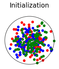
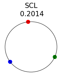
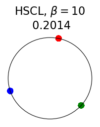
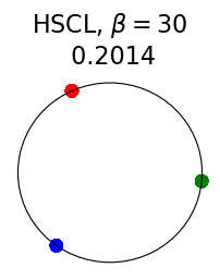
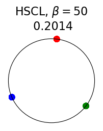
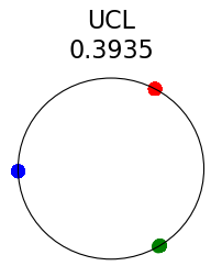
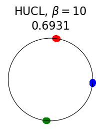
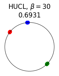
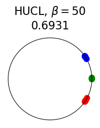
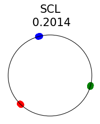
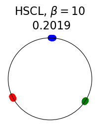
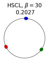
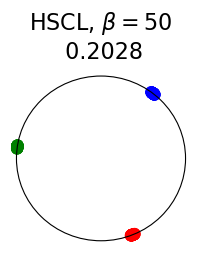
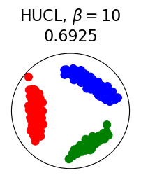
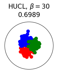
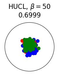
Figure 2 summarizes the results for synthetic data. For a representation function that achieves Neural-Collapse, the values of and across all values and the value of are , , and , respectively. These values are obtained by numerically evaluating the lower bounds in Theorem 2 and Theorem 3.
The first row in Figure 2 shows the result using label information for positive pair construction. The values of the minimum loss in different settings are displayed at the top of Fig. 2. Our simulation results are consistent with our theoretical results. After 200 training epochs, we observed that and across all values and converged to their minimum values. From the figure, we can visually confirm that the representations exhibit Neural-Collapse in , , and . However, Neural-Collapse was not observed in HUCL as the class means deviate significantly from the ETF geometry.
The second row in Figure 2 shows the results using the additive Gaussian noise augmentation mechanism, where label information is not used in constructing positive examples. We note that in accordance with our theoretical results, NC is observed in and . However, NC is not observed in and , likely due to the lack of conditional independence. Moreover, the degree of deviation from NC increases progressively with increasing hardness levels.
Contrary to a widely held belief that hard-negative sampling is beneficial in both supervised and unsupervised contrastive learning, results on this simple synthetic dataset suggest that not only may SCL not benefit from hard negatives, but UCL may suffer from it. To investigate whether these conclusions hold true more generally or whether there are practical benefits of hard-negatives for SCL and UCL, we turn to real-world datasets next.

5.2 Results for real data
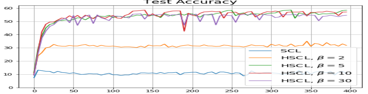
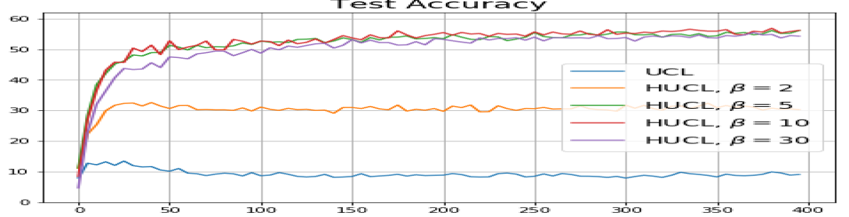
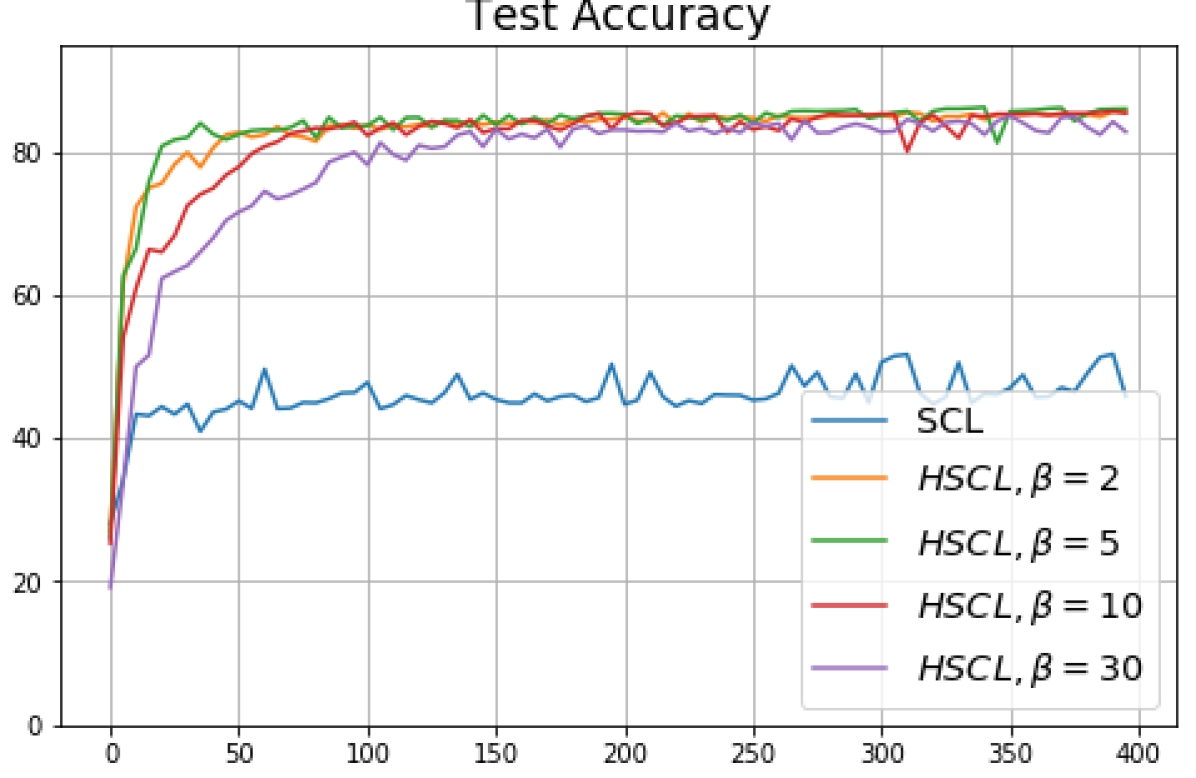
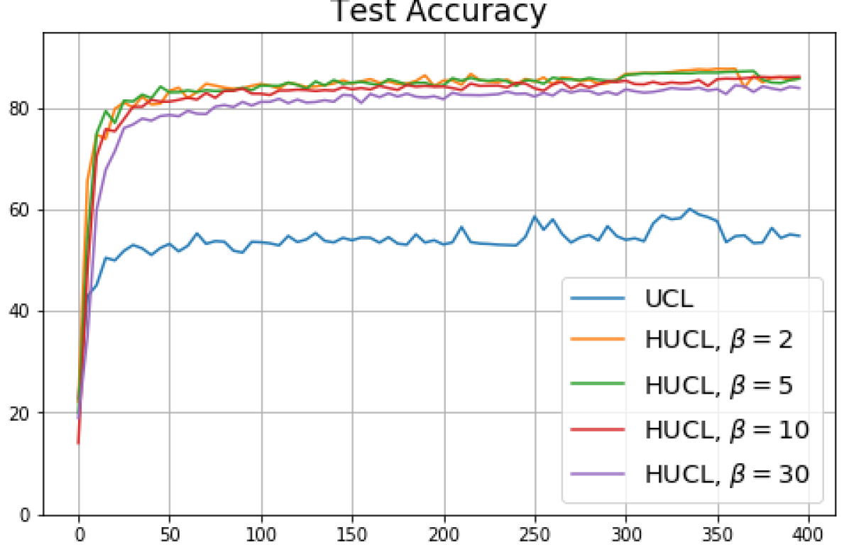
We first show that hard-negative sampling improves downstream classification performance. From the first row of Fig. 3, we see that with negative sampling at moderate hardness levels (), the classification accuracies of HSCL and HUCL are more than points higher than those of SCL and UCL respectively.
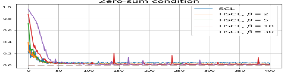
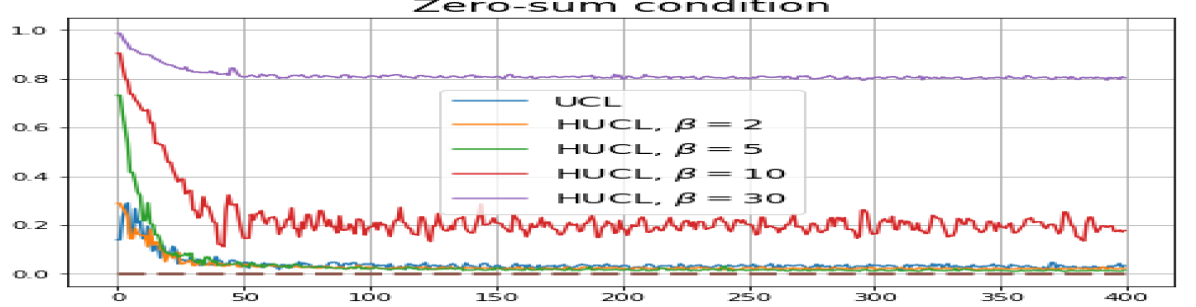
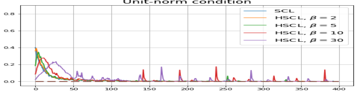
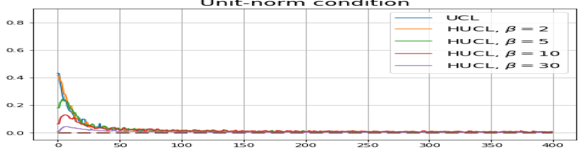
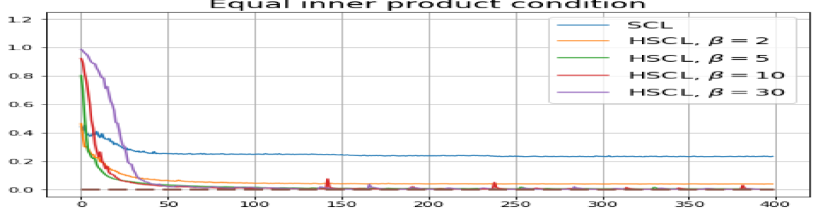
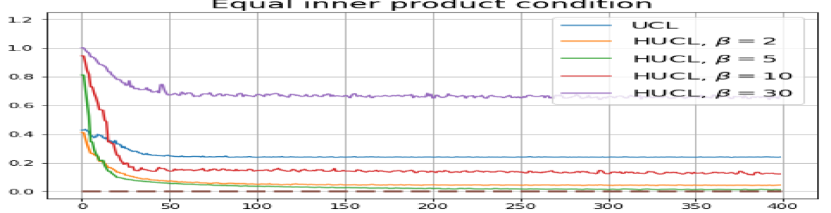
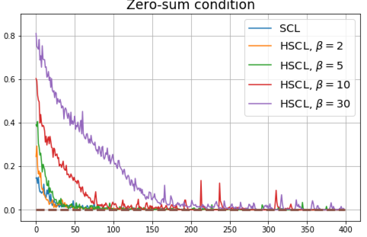
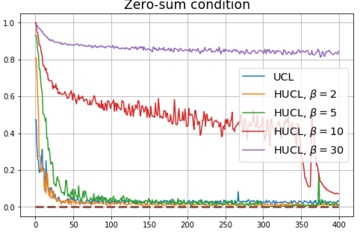
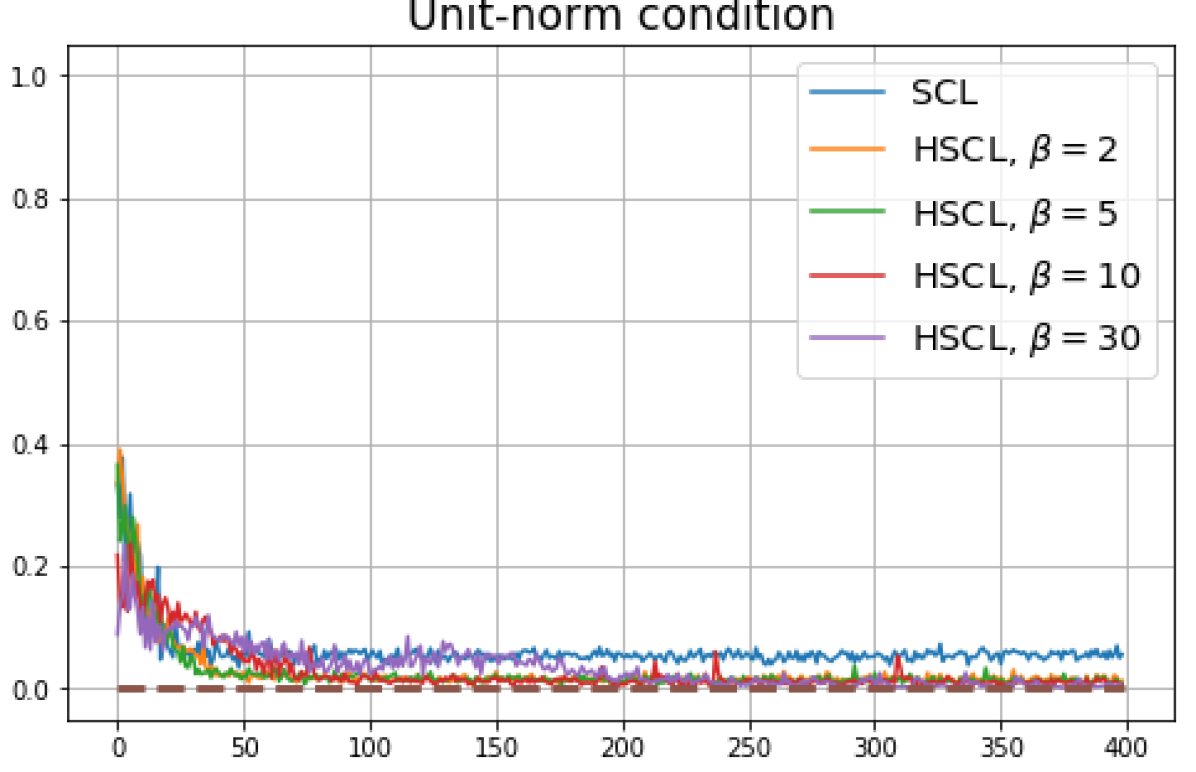
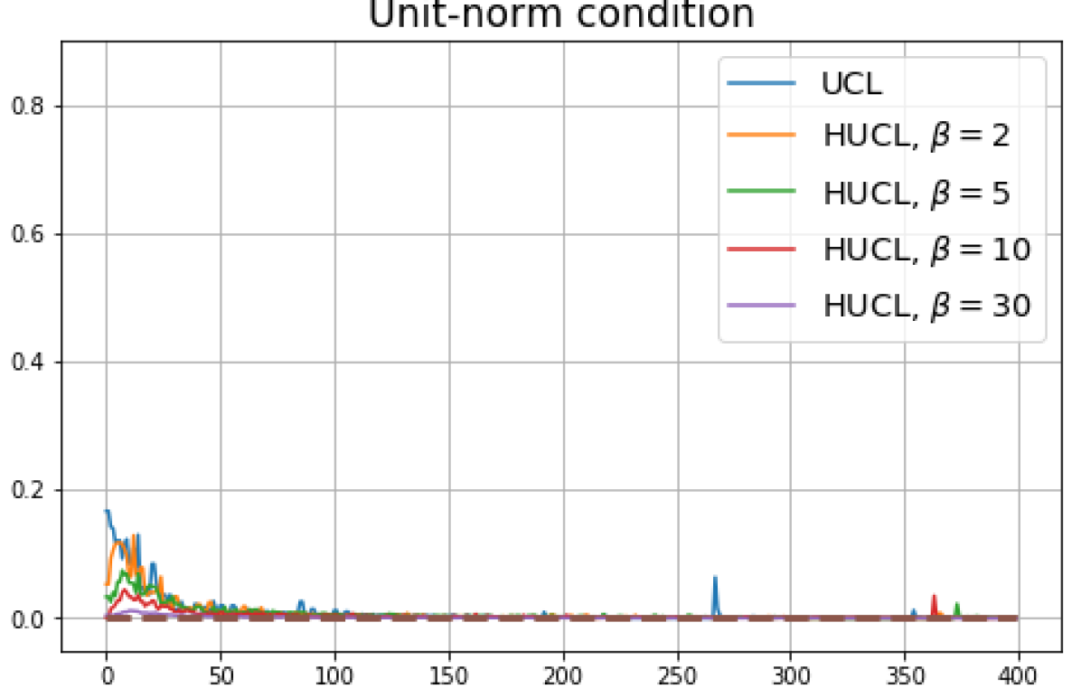
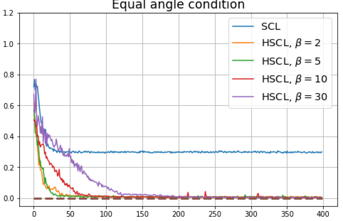
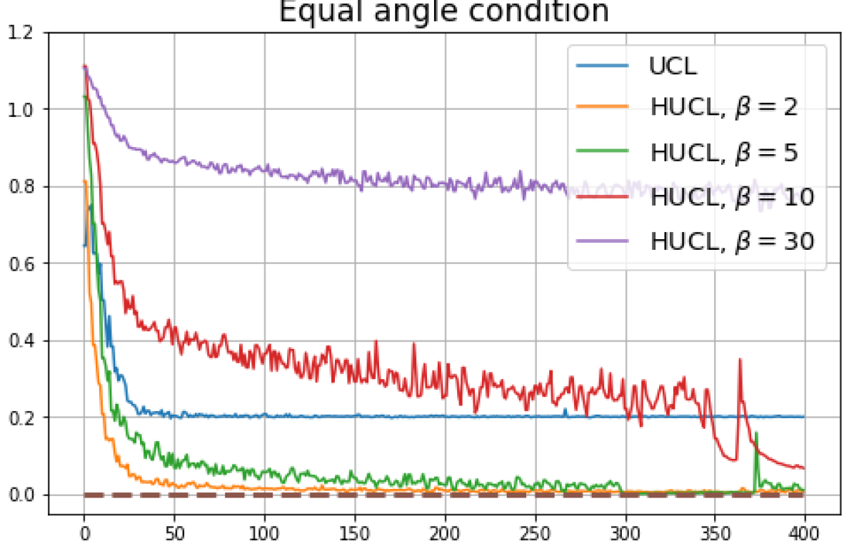
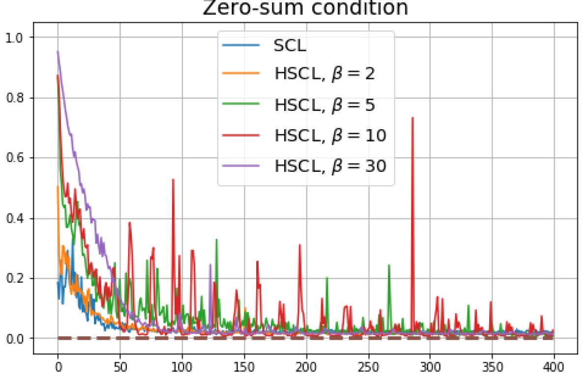
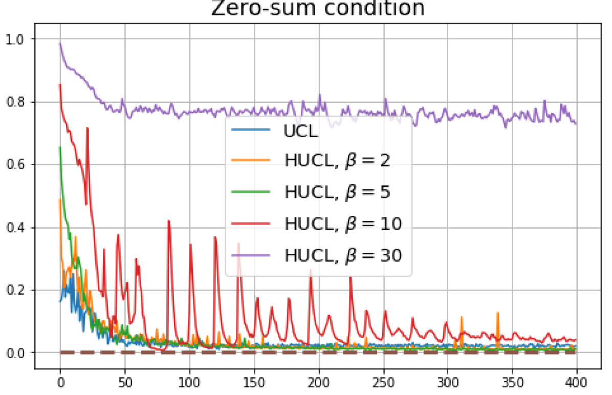
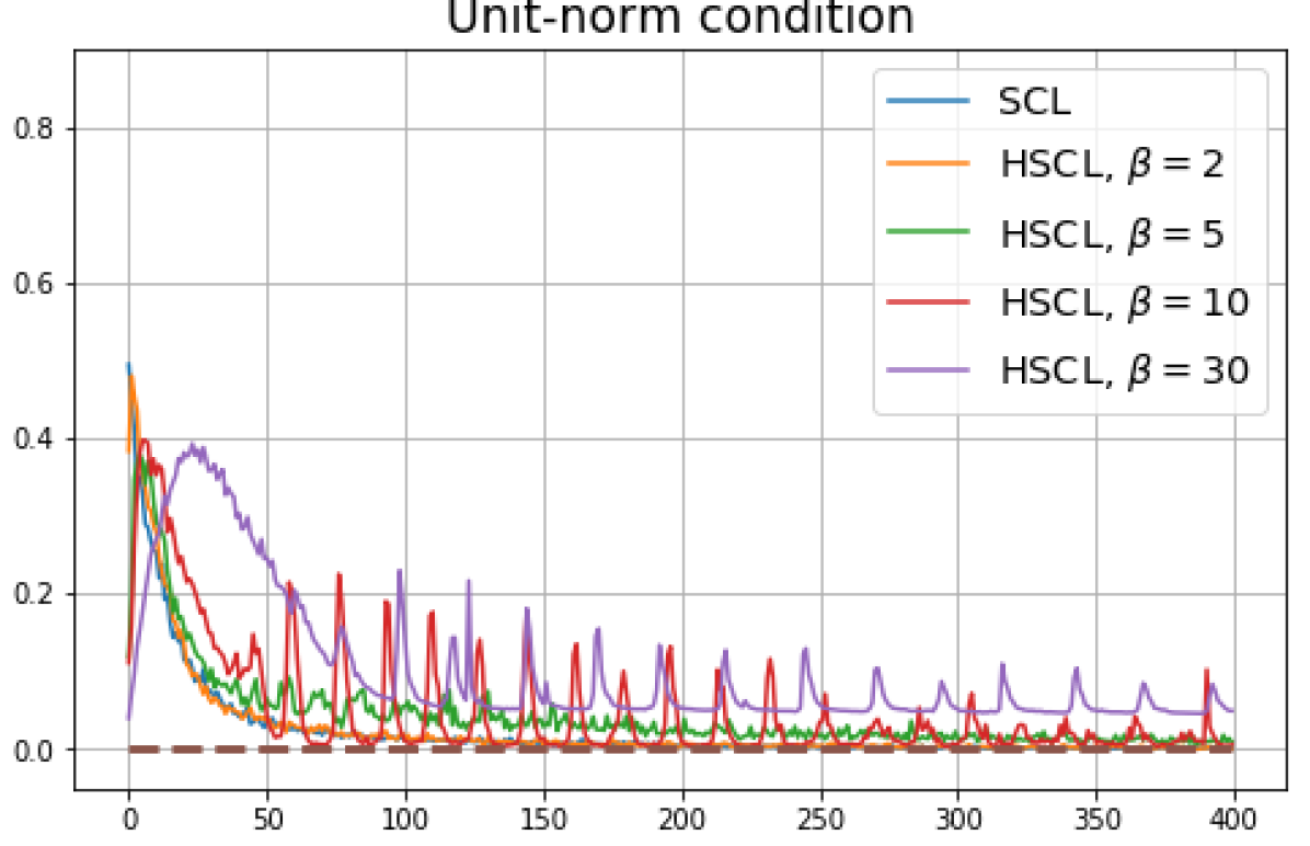
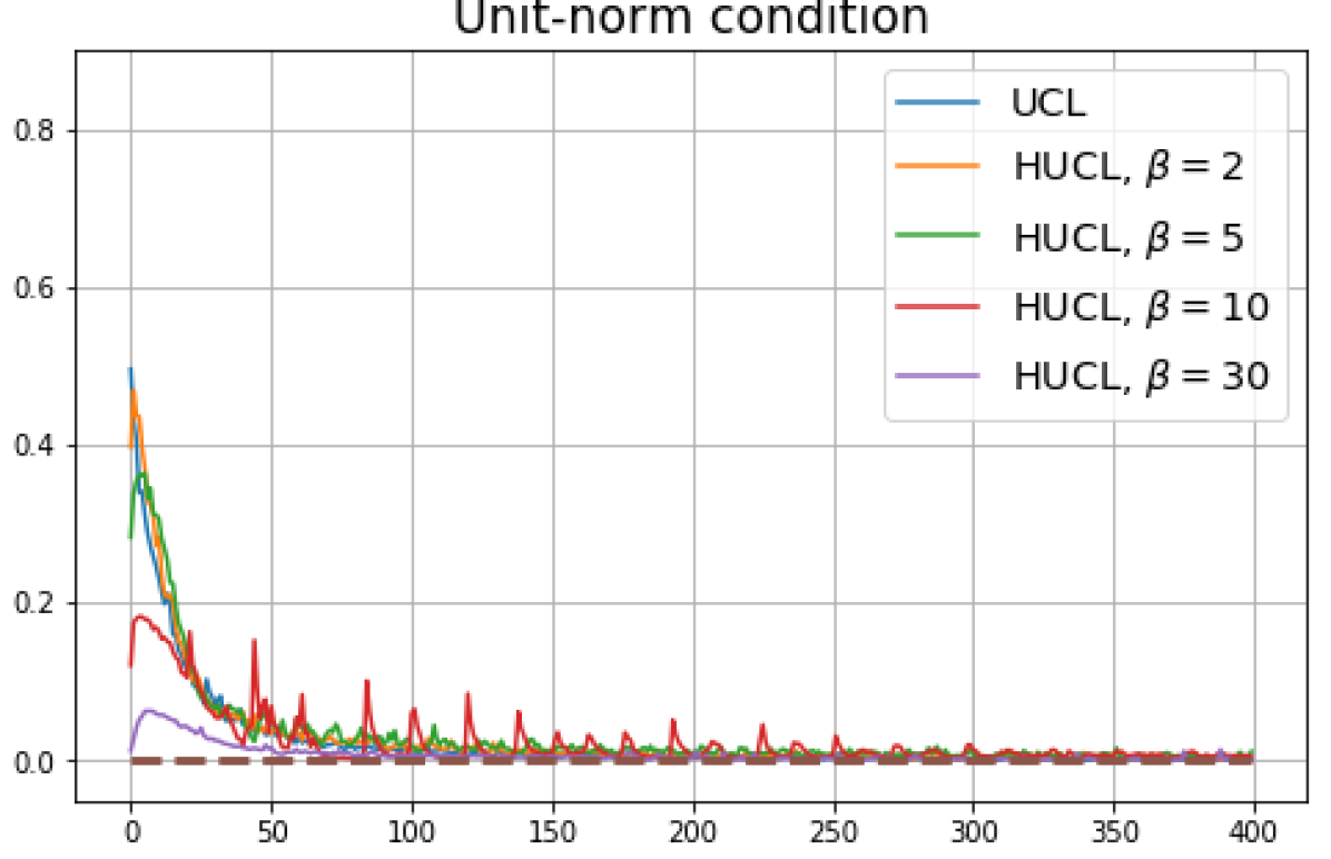
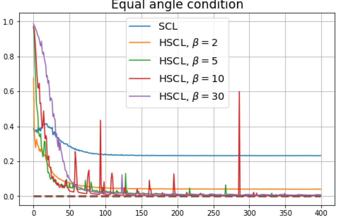
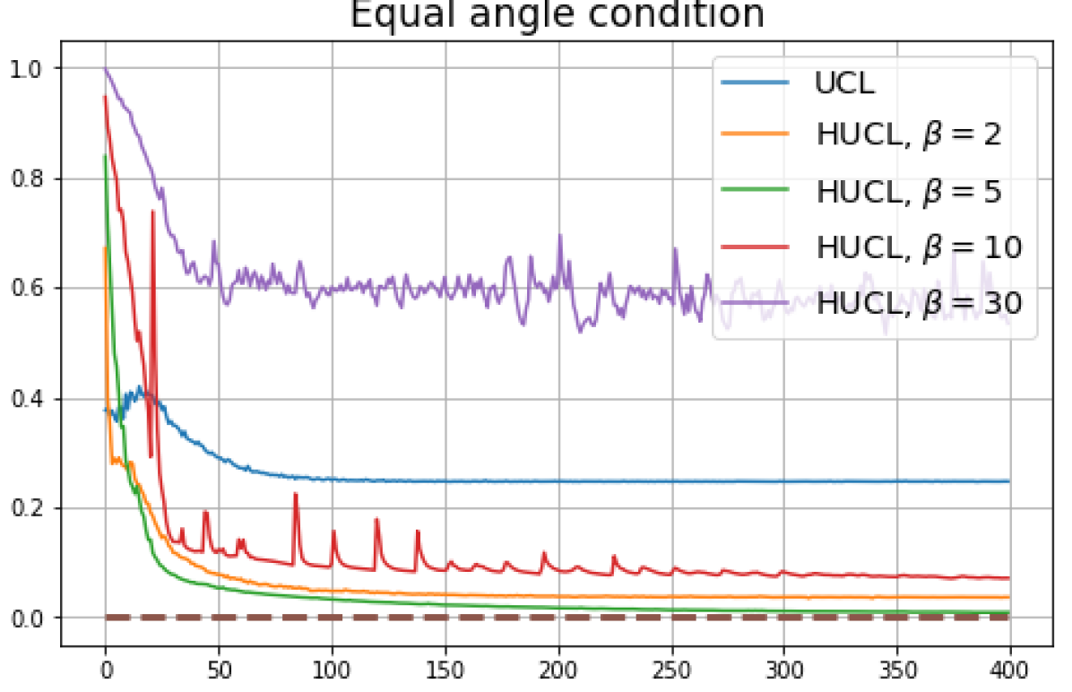
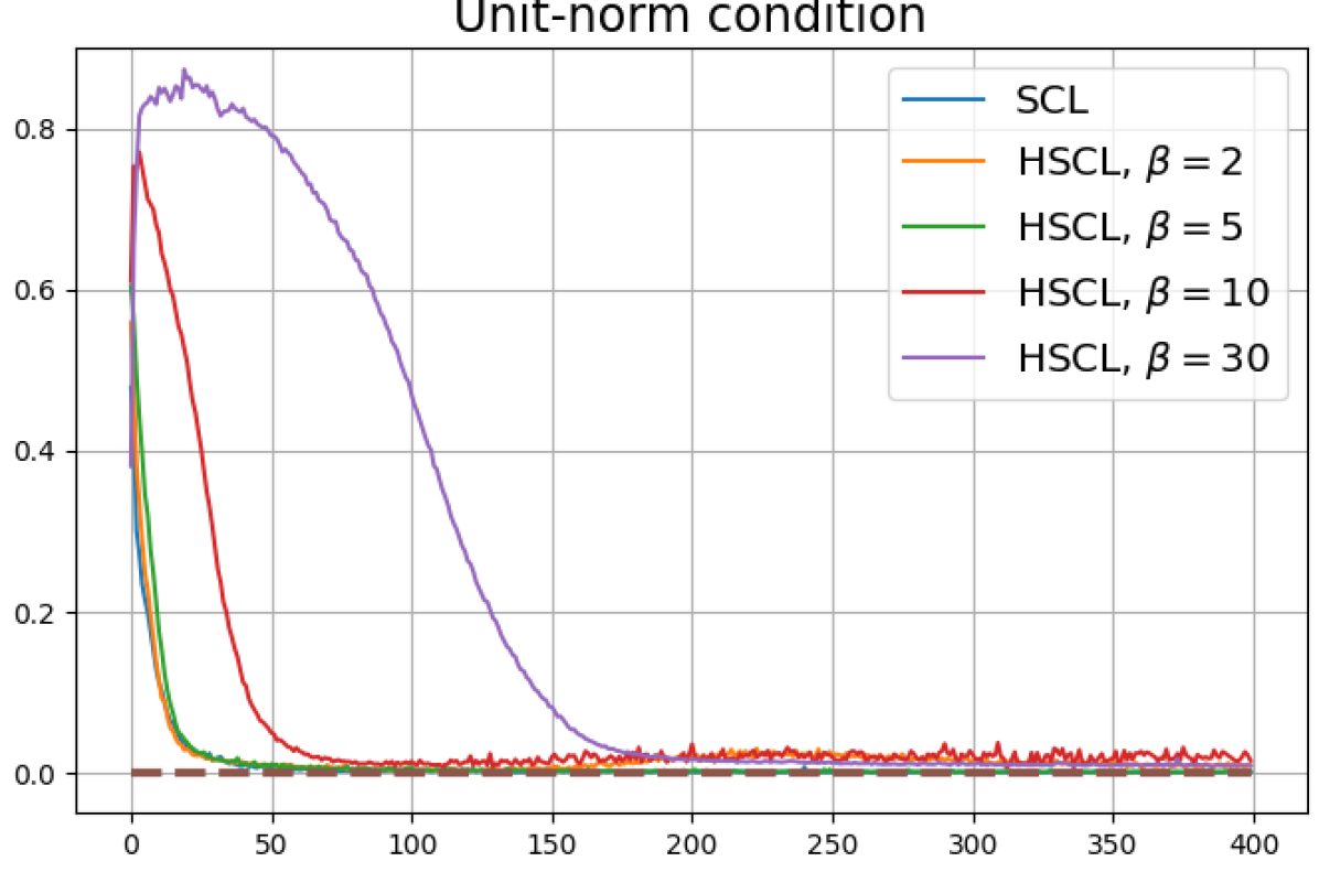
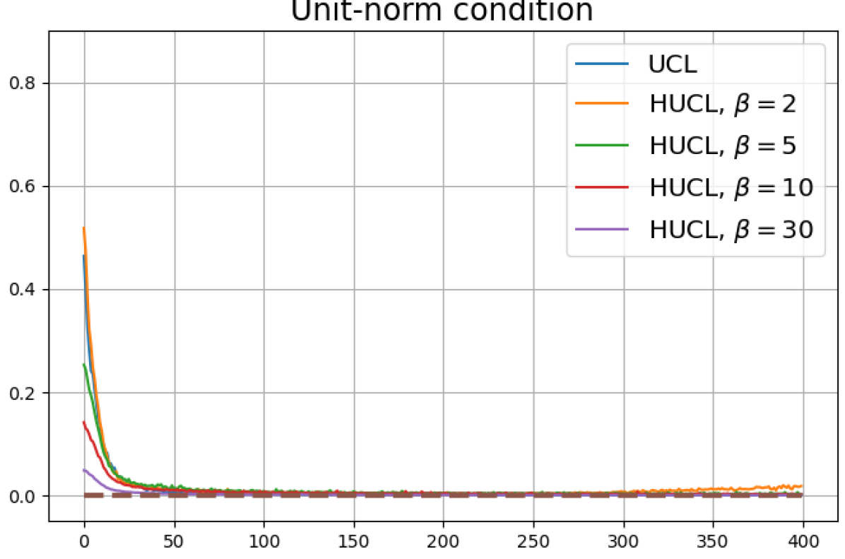
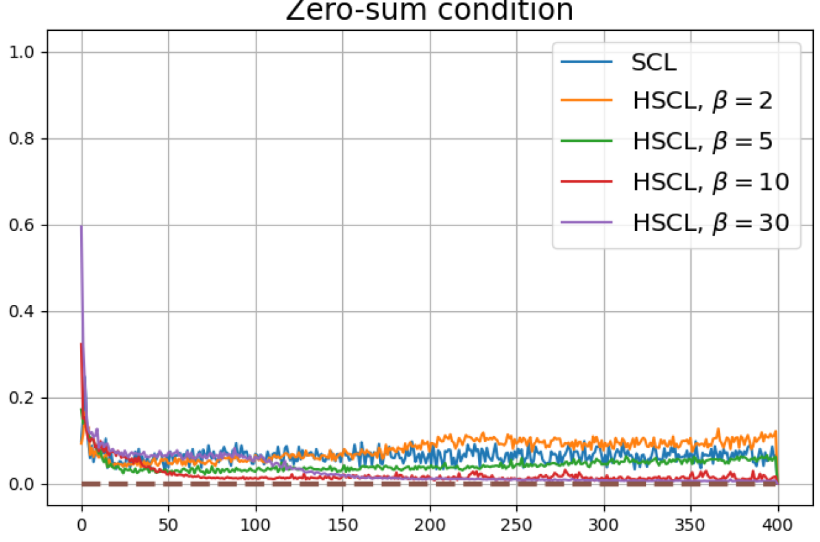
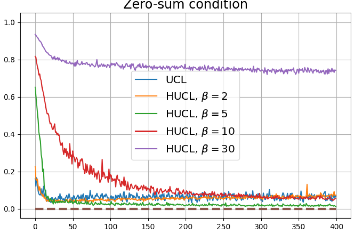
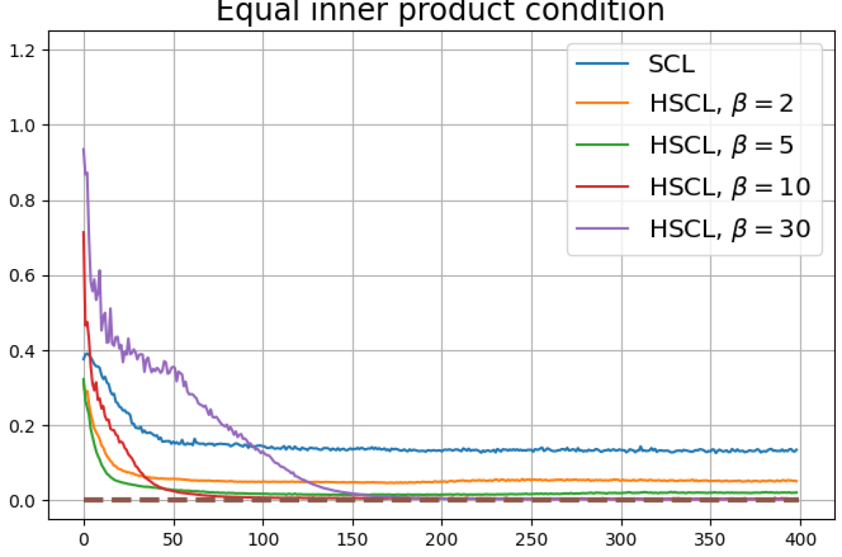
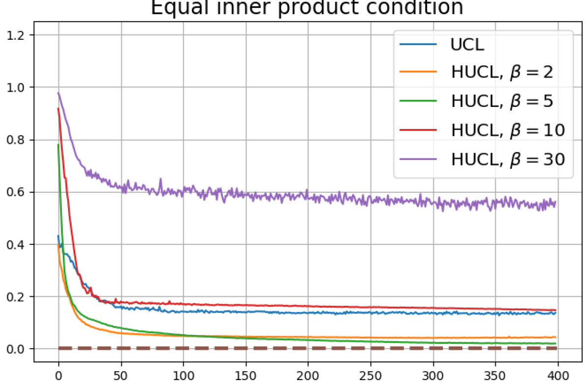
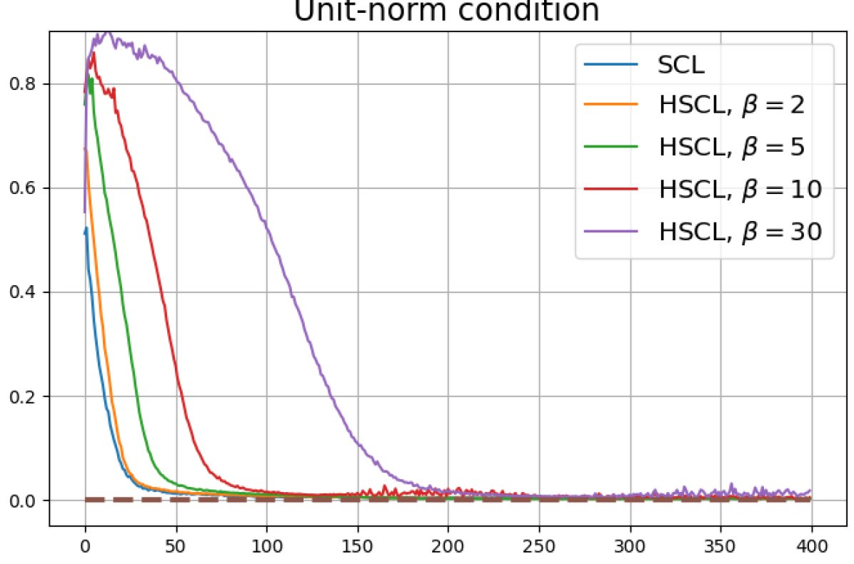
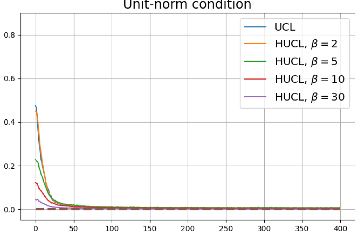
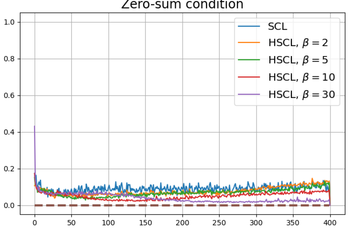
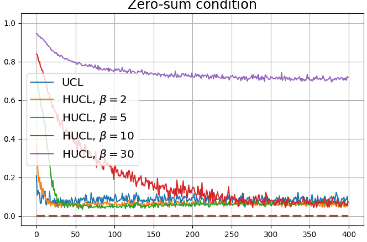
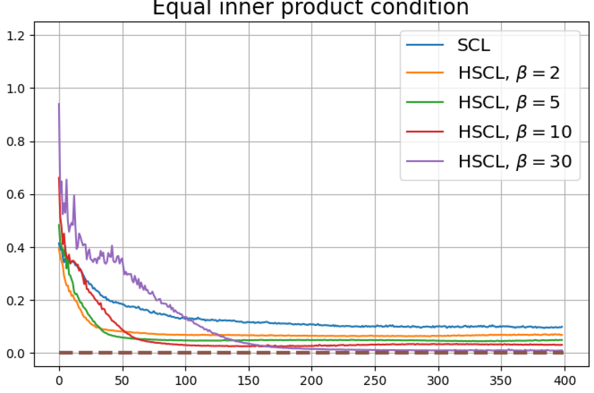
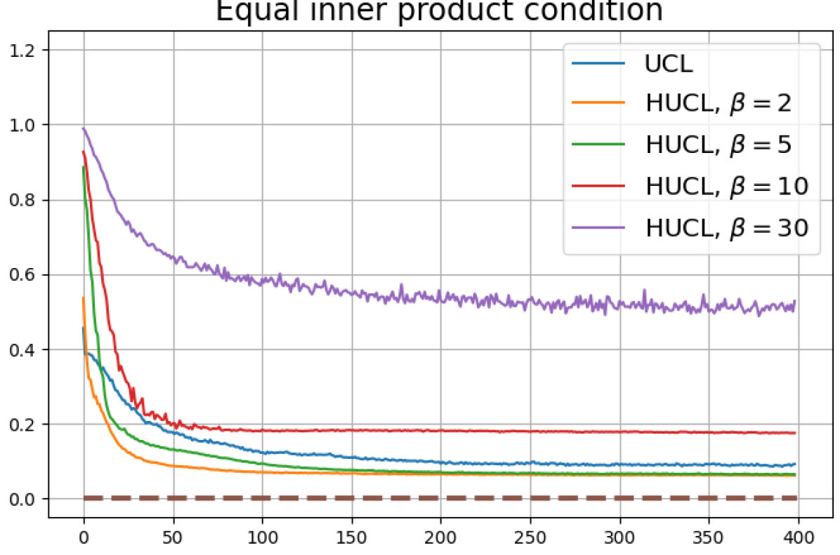
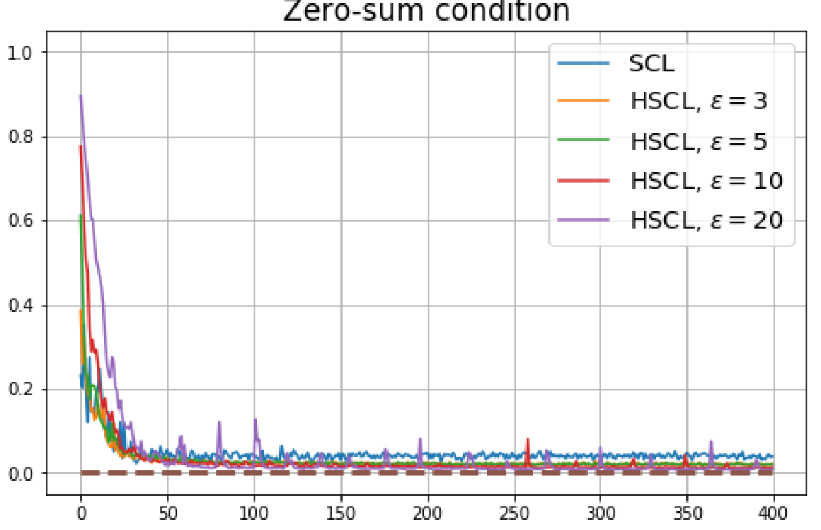
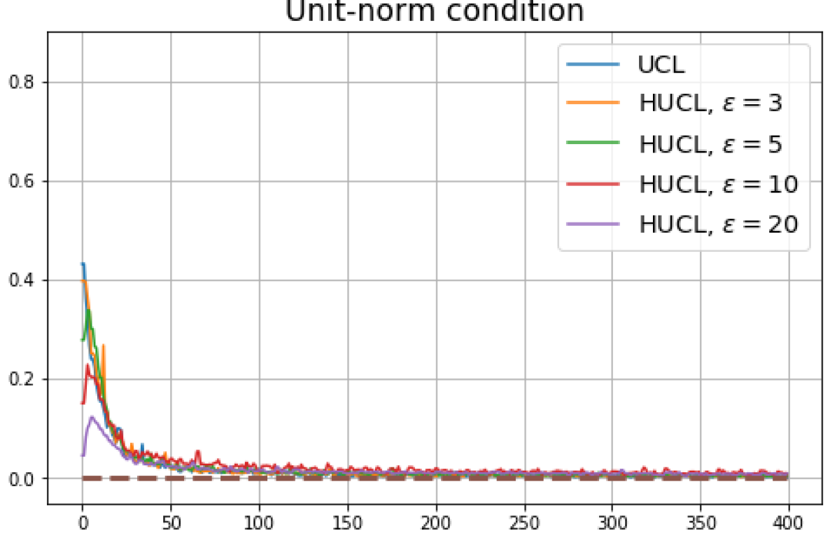
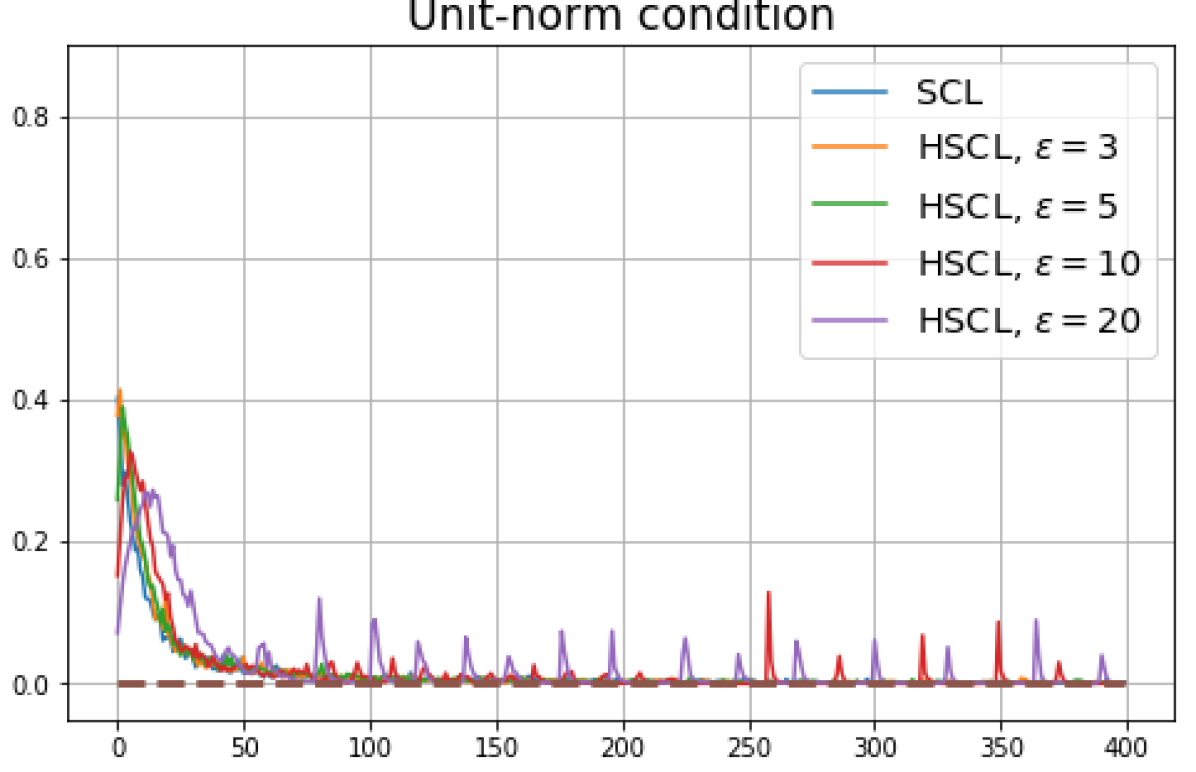
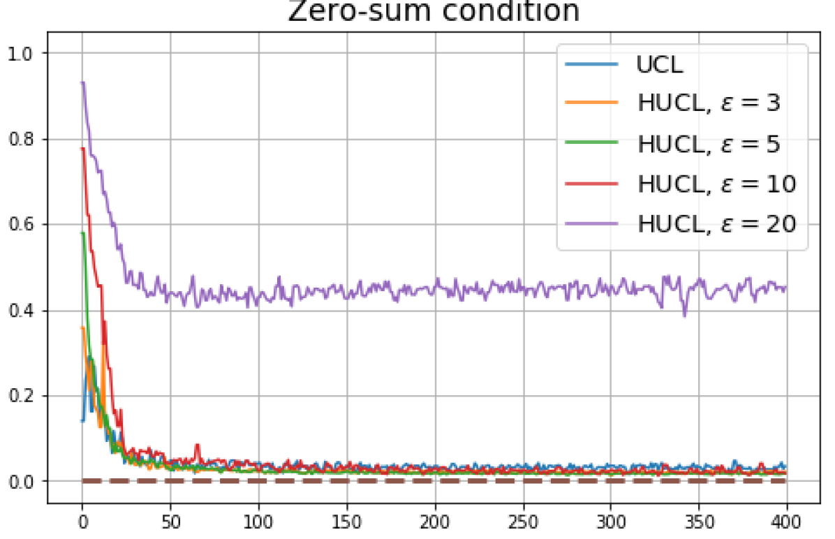
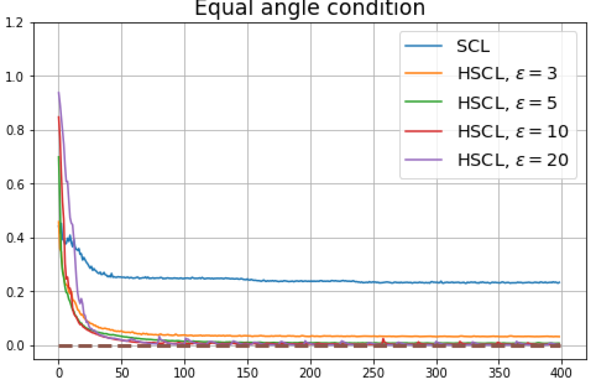
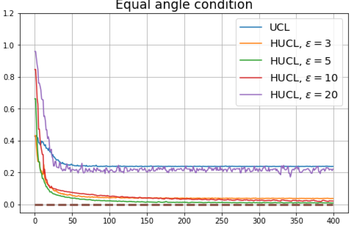
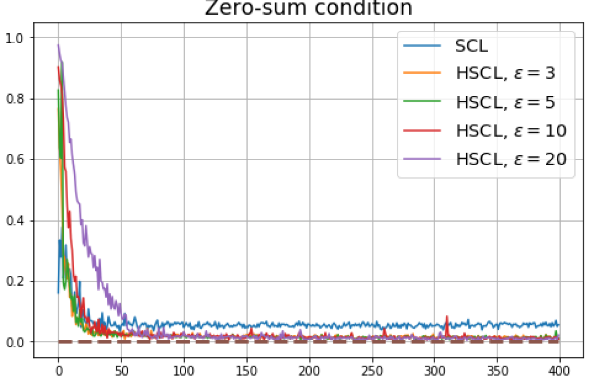
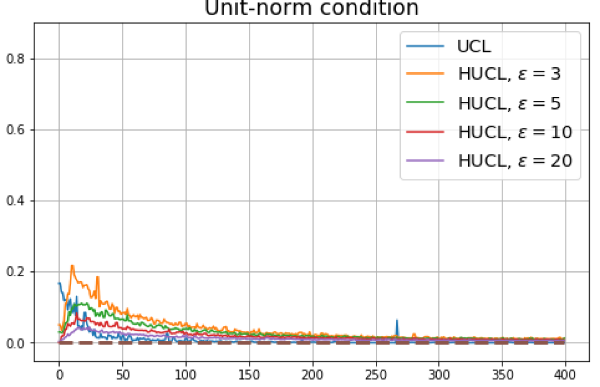
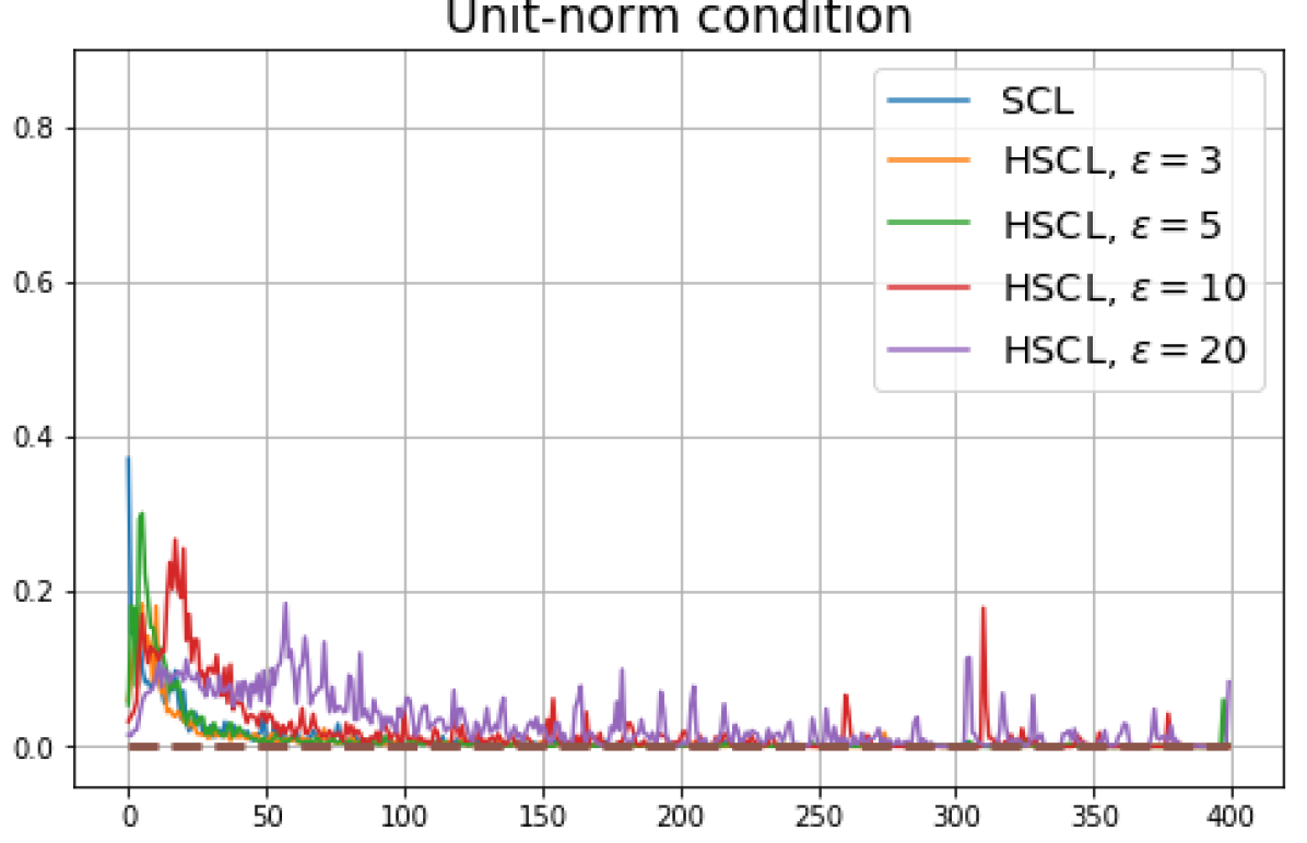
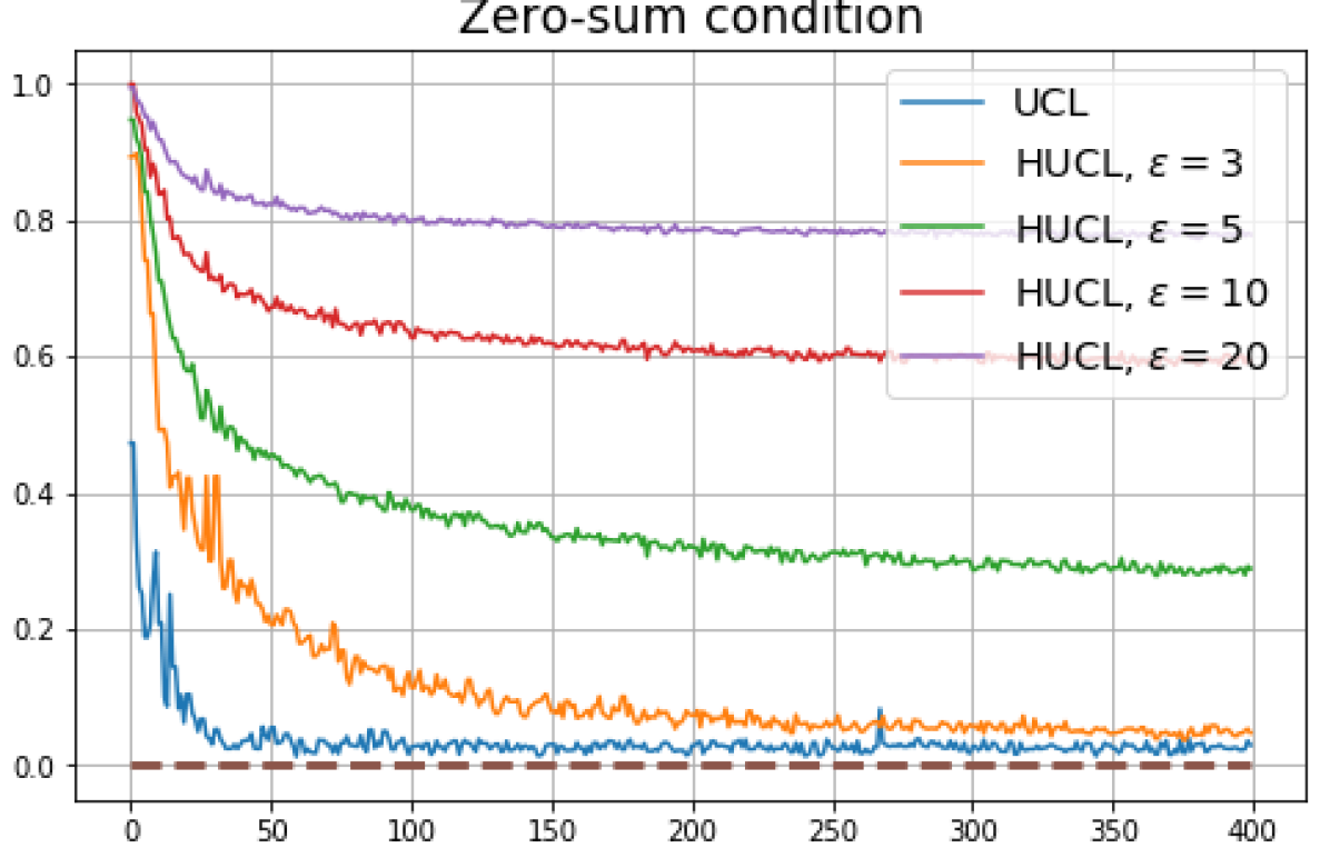
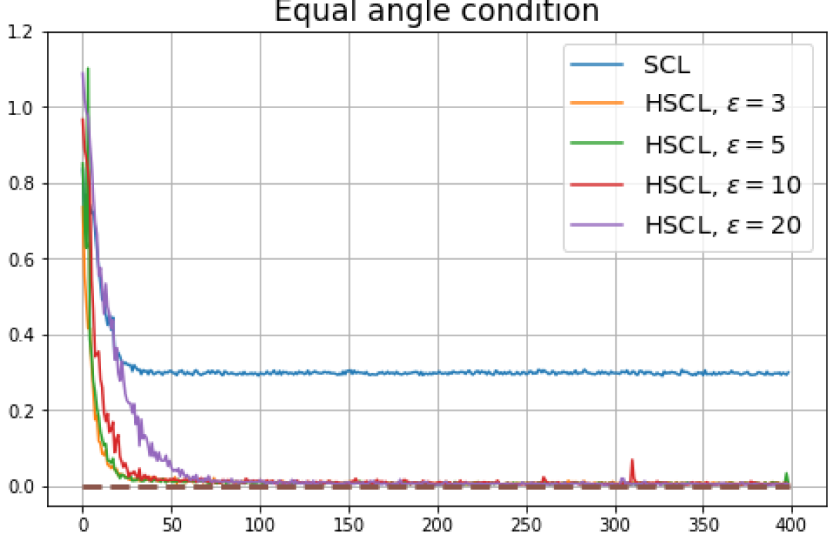
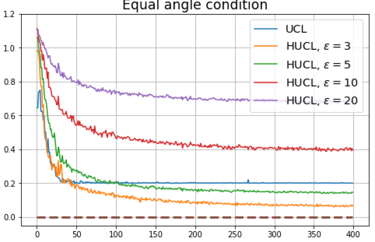
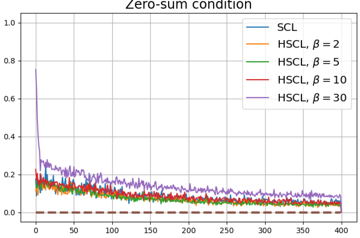
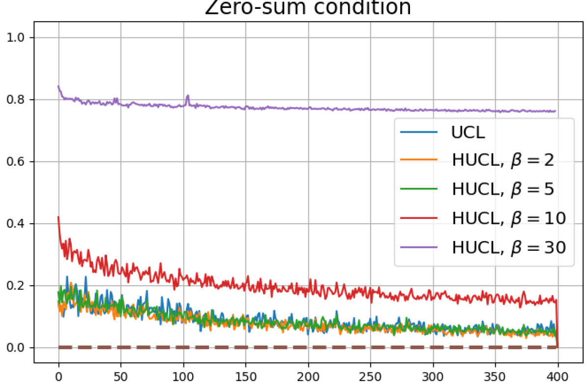
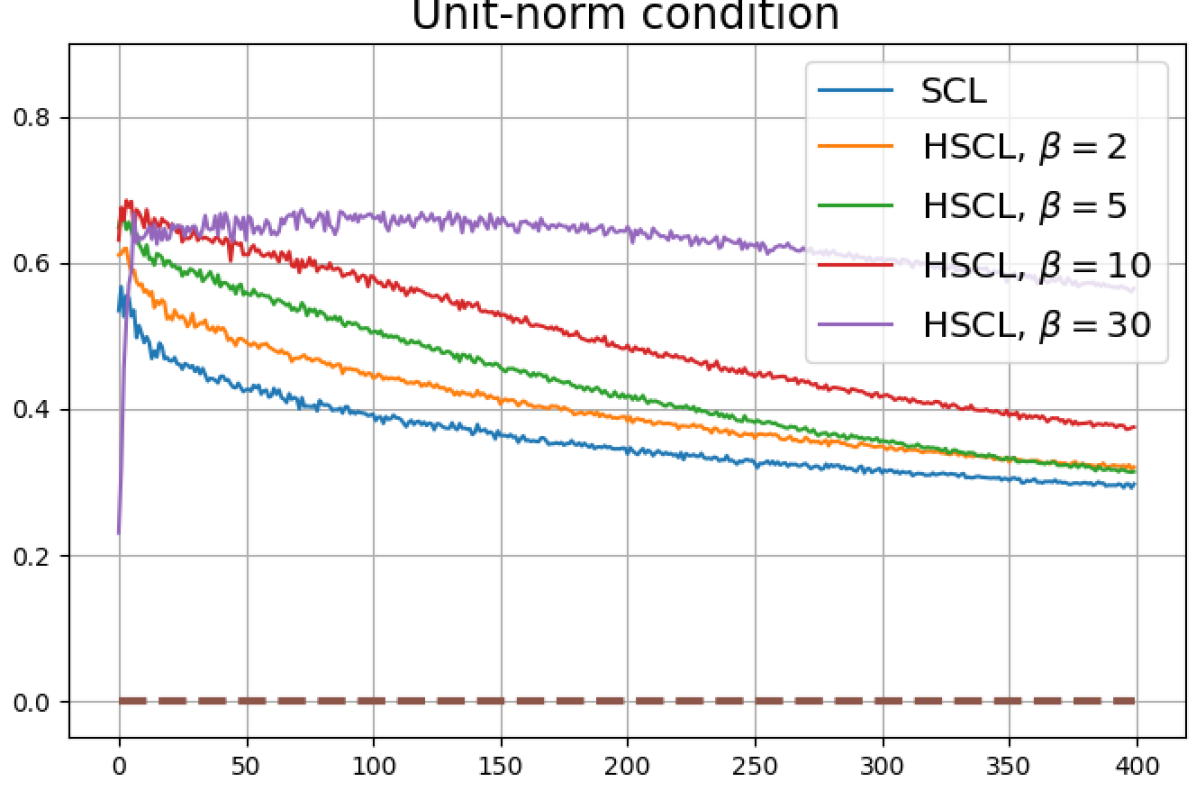
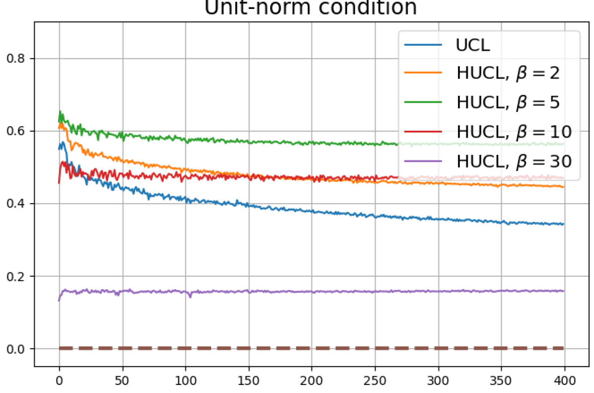
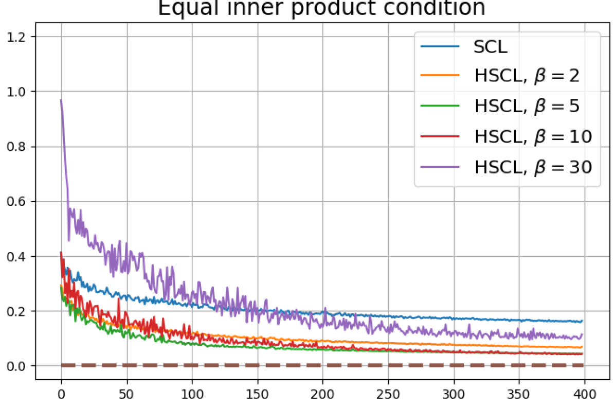
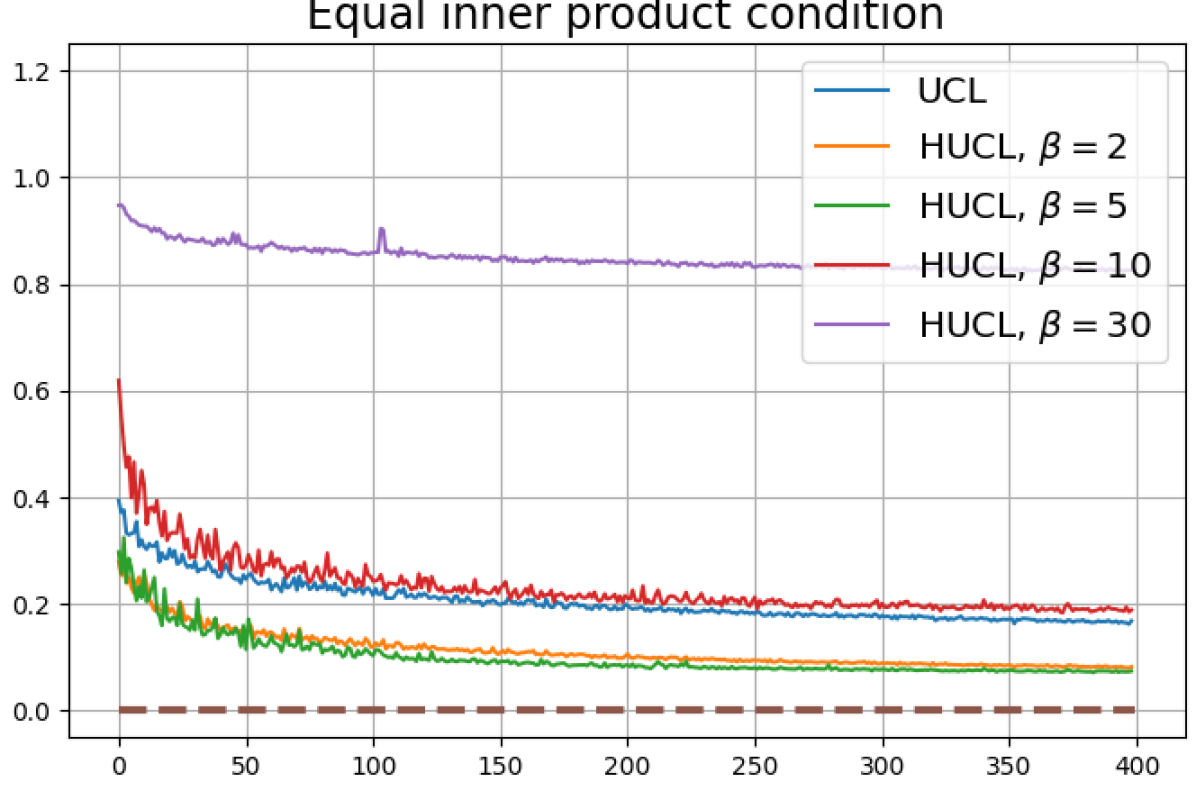
Achievability of Neural-Collapse: We investigate whether SCL and UCL losses trained using Adam can attain the globally optimal solution exhibiting NC. To test this, in line with properties and condition (13) in Theorems 2 and 3, we employ the following metrics which are plotted in Fig. 3 in rows two through four.
-
1.
Zero-sum metric:
-
2.
Unit-norm metric:
-
3.
Equal inner-product metric:
We note that even though the equal inner-product class means condition together with unit-ball normalization implies the zero-sum and unit-norm conditions, we report these three metrics separately to gain more insight.
According to Theorems 2 and 3, the optimal solutions for UCL, SCL, and HSCL are anticipated to manifest NC. However, our experimental findings reveal a gap between the theoretical expectations and the observed outcomes. Specifically, in both supervised and unsupervised settings, when leveraging the random negative sampling method, i.e., when the negative samples are sampled uniformly from the whole data in a mini-batch which may include the anchor and positive samples, NC is not exactly achieved: the zero-sum and equal inner-product metrics do not approach zero for all hardness levels (rows 2 and 4 in Fig. 3). This is also supported by the results in Table 1 which shows the theoretical minimum SCL loss value and the practically observed SCL loss values after epochs for different hardness levels. While our theoretical results posit that both SCL and HSCL should have the same minimum loss value for all values of , the practically observed loss value for SCL deviates noticeably from theory. On the other hand, increased hardness in HSCL, especially at , brings the observed loss value close to the theoretical minimum.
| Theory | Empirical | ||||
| 0.3105 | SCL | HSCL | |||
| 0.3384 | 0.3603 | 0.3106 | 0.3107 | 0.3222 | |
In addition, the manner in which the final values of NC metrics change with increasing hardness levels is qualitatively different in the supervised and unsupervised settings. Specifically, in the supervised settings, increased hardness invariably leads to improved results, and the model tends to approach NC, notably at . However, in the unsupervised settings, there seems to be just a single optimal hardness level ( is best among the choices tested).
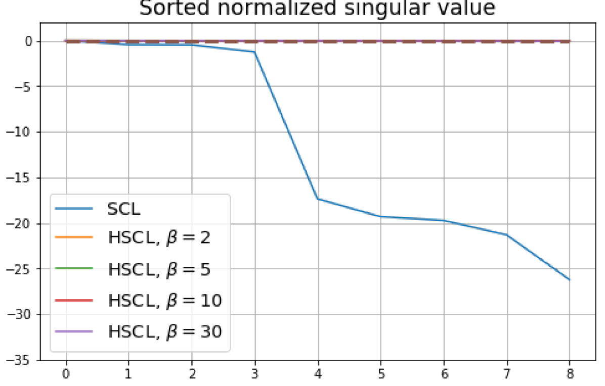
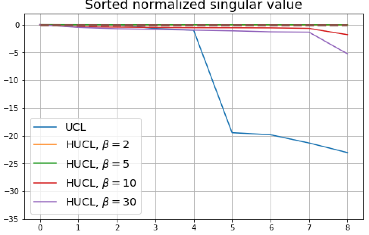
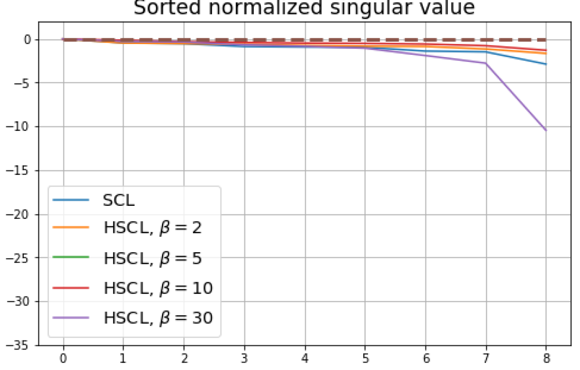
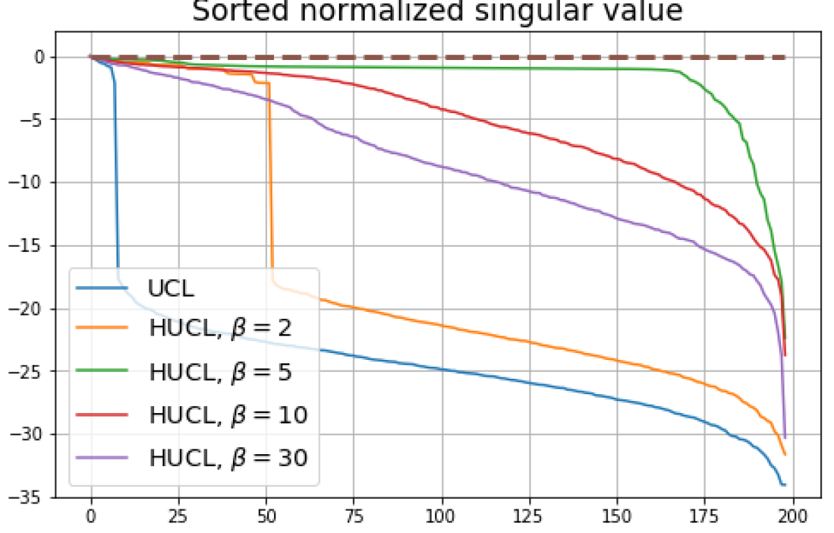
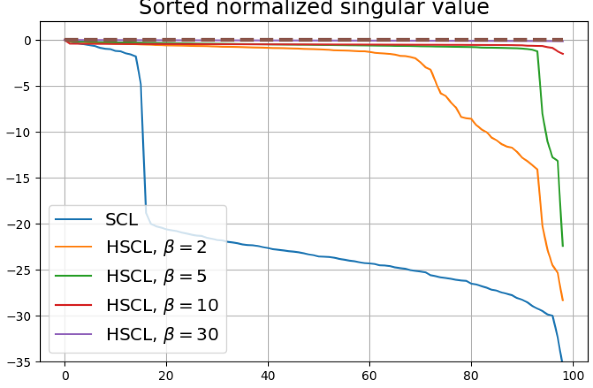
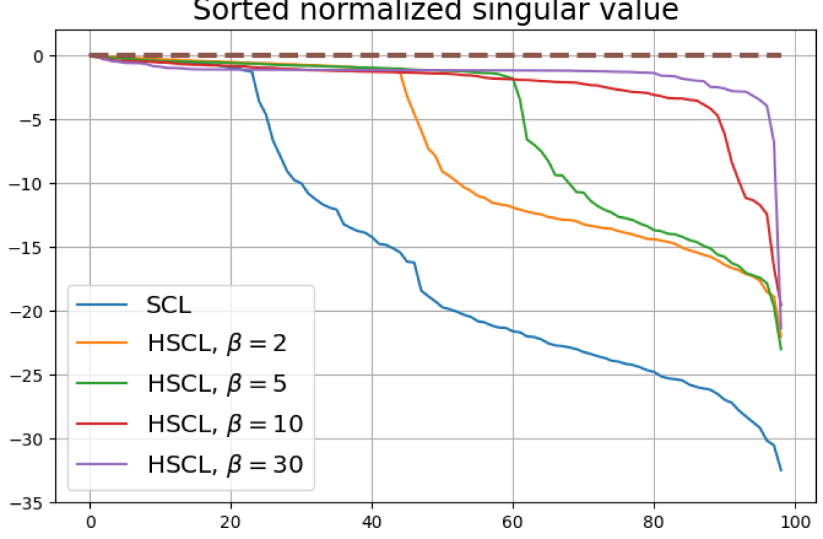
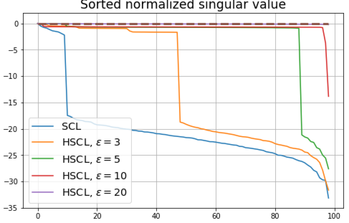
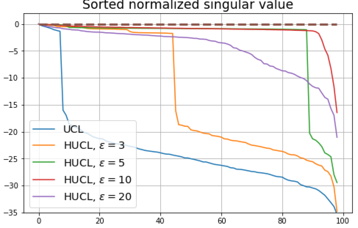
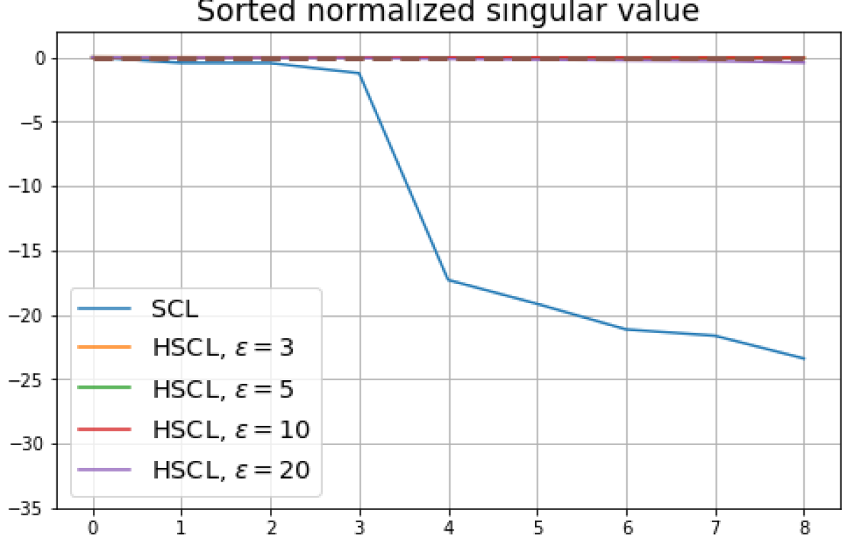
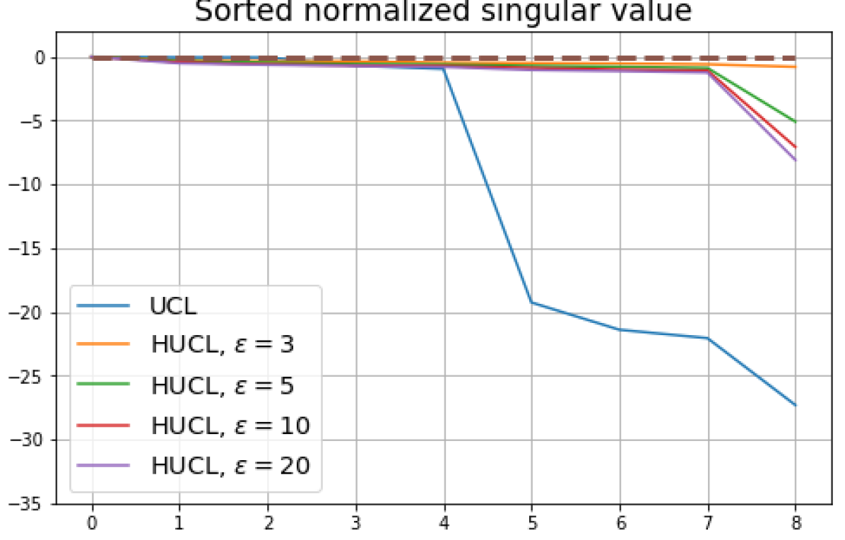
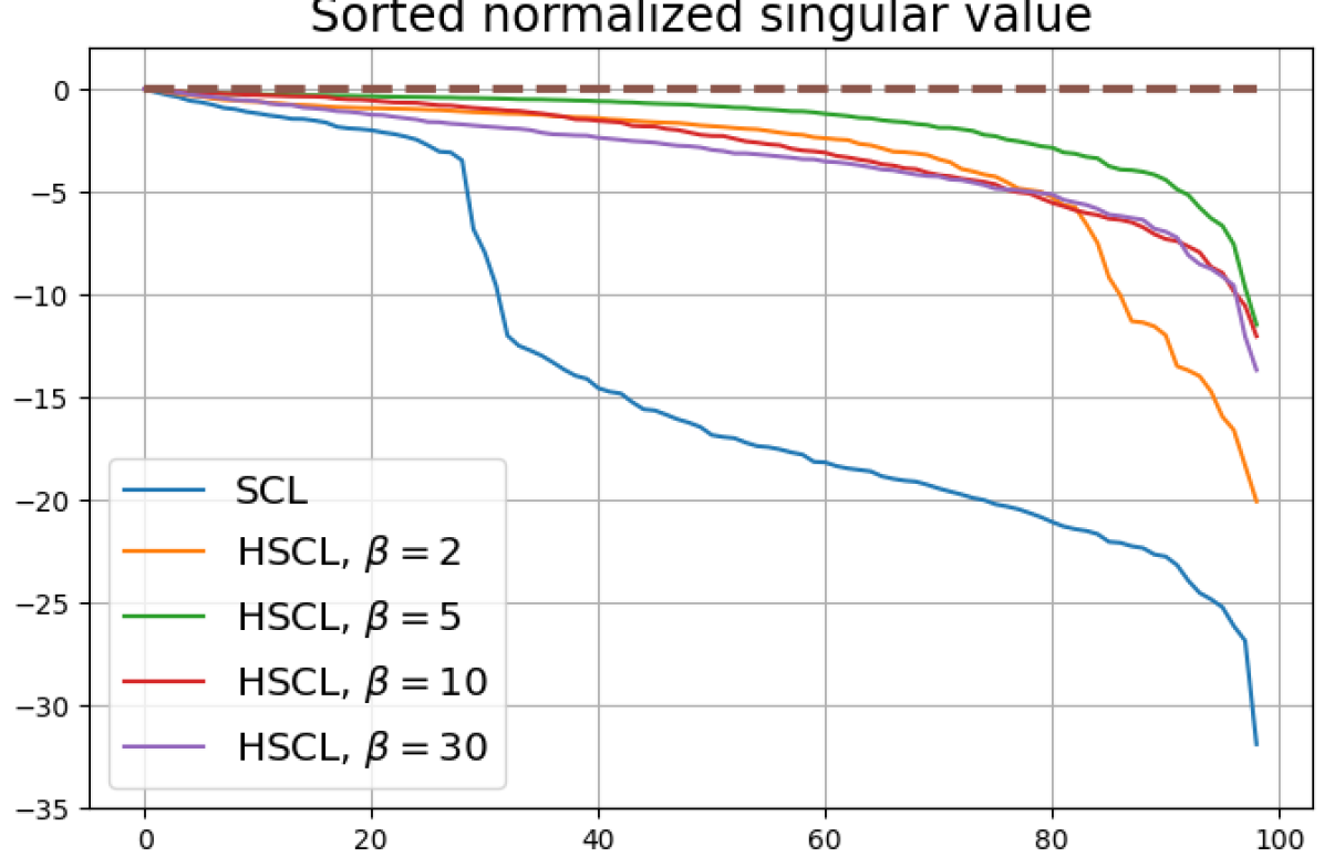
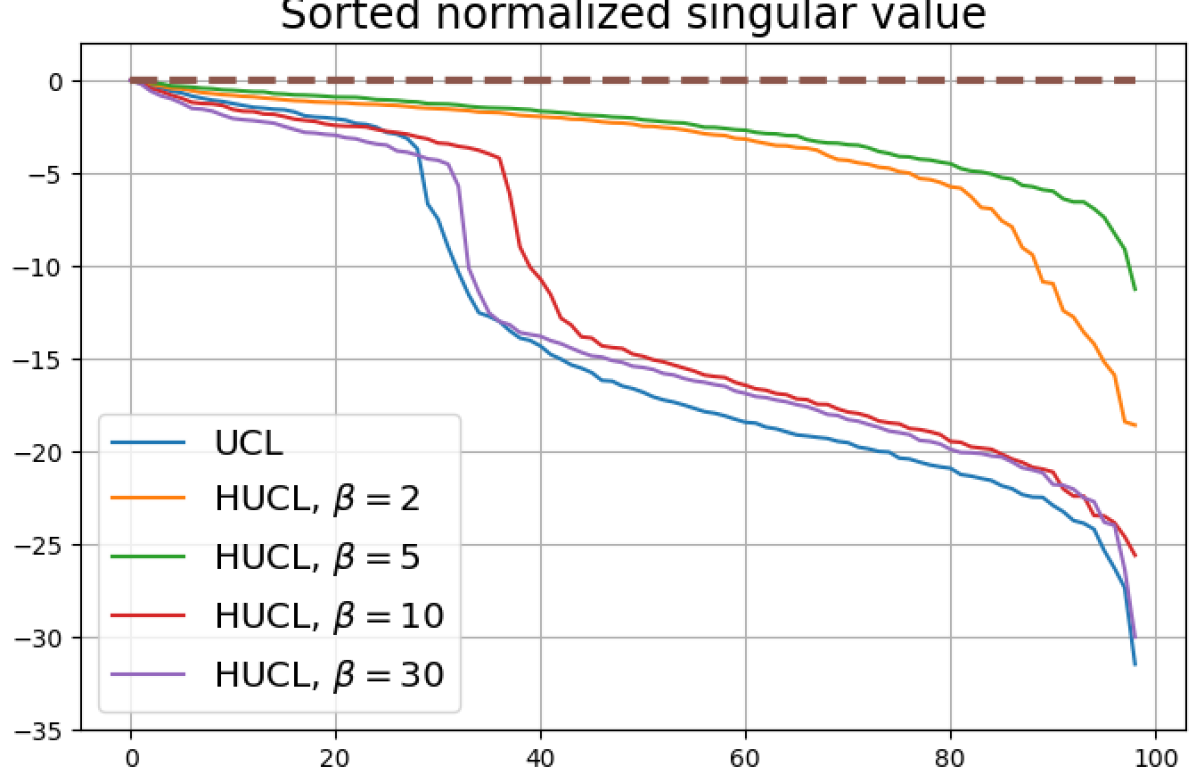
5.3 Dimensional-Collapse
To gain further insights, we investigate the phenomenon of Dimensional-Collapse (DC) that is known to occur in contrastive learning (see [12]).
Definition 7.
[Dimension Collapse (DC)] We say that the class means suffer from DC if their empirical covariance matrix has one or more singular values that are zero or orders of magnitude smaller than the largest singular value.
If , then under Neural-Collapse (NC), the class mean vectors would have full rank in representation space since they form an ETF (see Definition 5). Thus when , . However, we note that because, for example, the class means could have full rank and satisfy the equal inner-product and unit-norm conditions in Theorem 2 without satisfying the zero-sum condition.
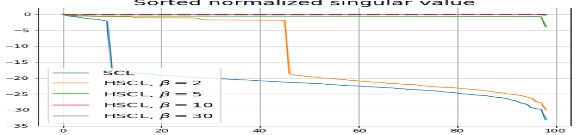
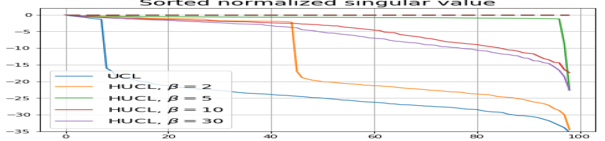
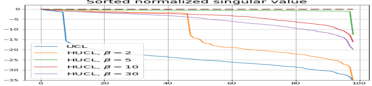
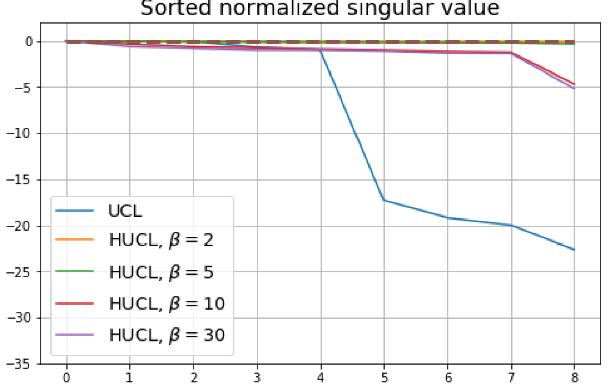
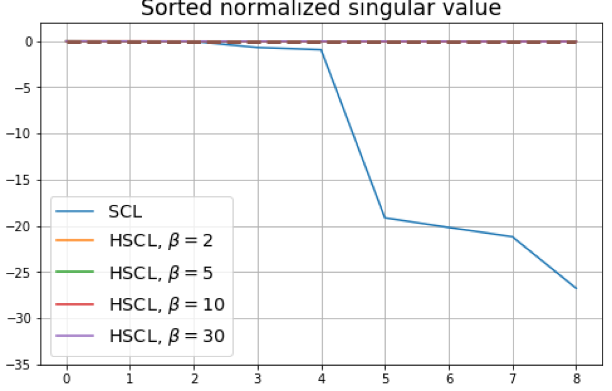
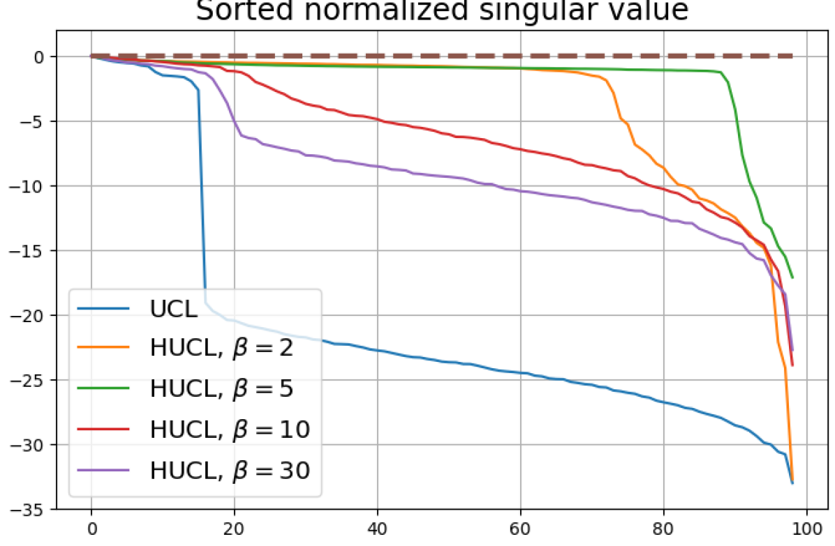
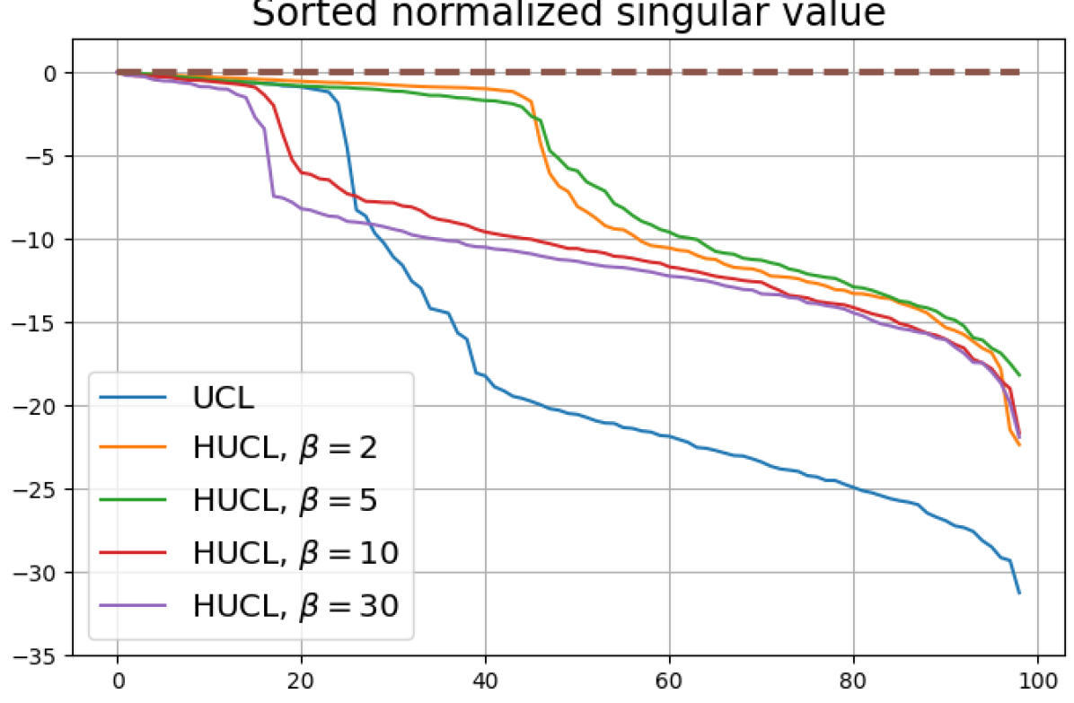
We numerically assess DC by plotting the singular values of the empirical covariance matrix of the class means (at the end of training) normalized by the largest singular value in decreasing order on a log-scale. Results for UCL, SCL, HUCL, and HSCL are shown in Fig. 4. In the supervised settings, (first row and first column of Fig. 4), the results align with our previous observations from Fig. 3. However, in the unsupervised settings (first row and second column of Fig. 4), while HUCL with high hardness values deviates more from NC compared to UCL in Fig. 3, in Fig. 4 we see that HUCL suffers less from DC.
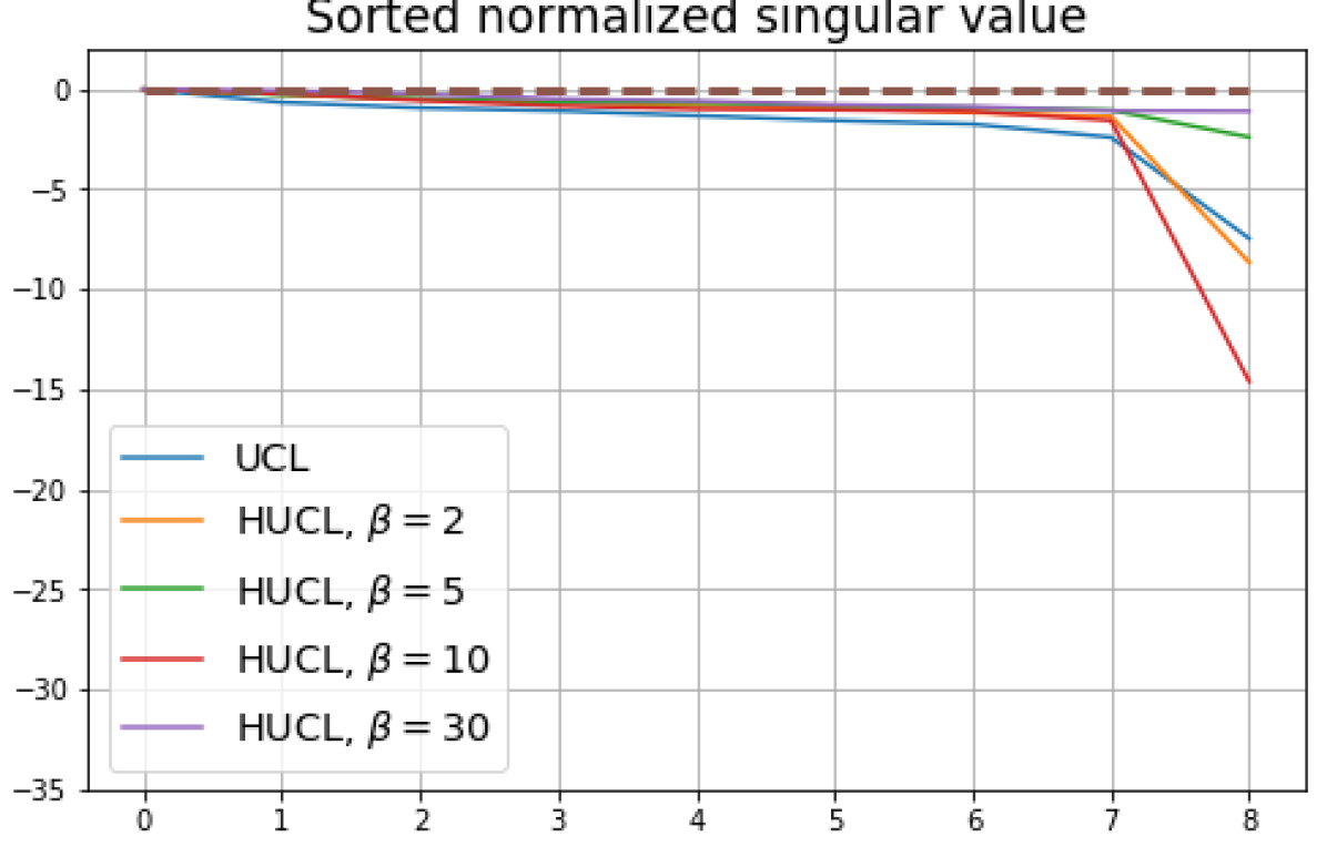
5.4 Role of initialization
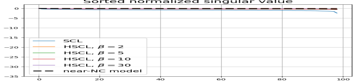
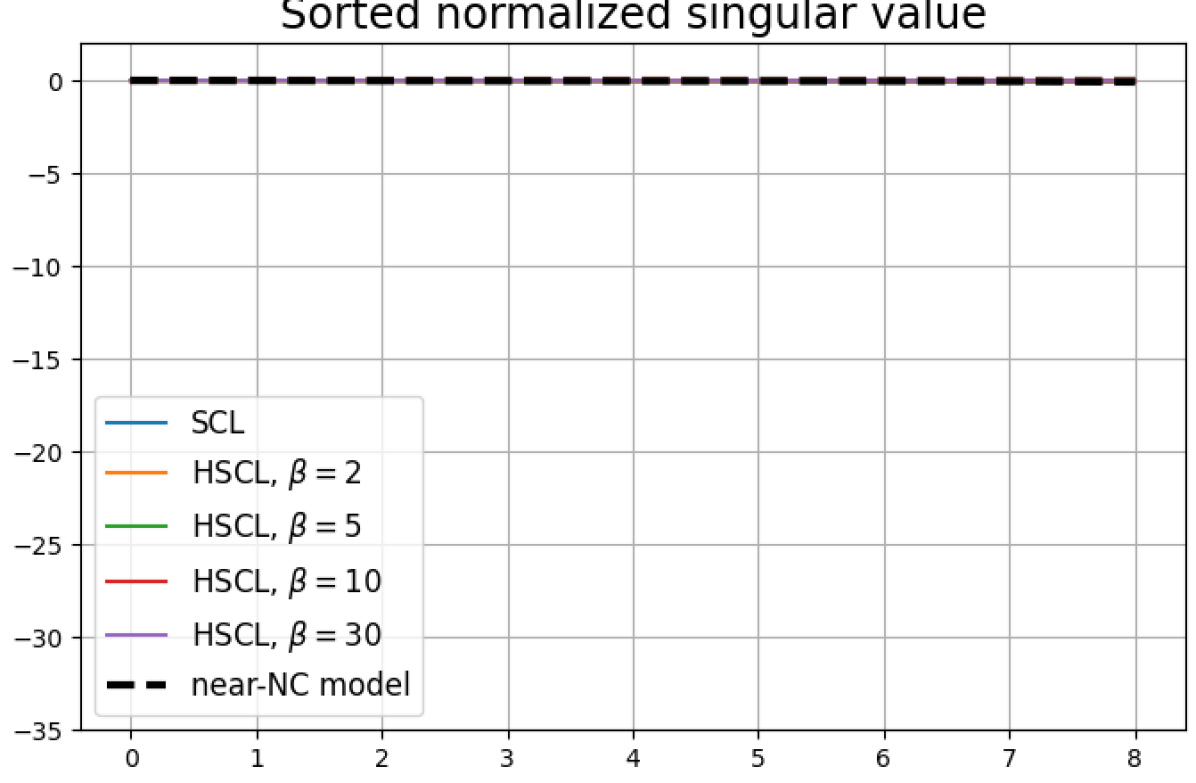
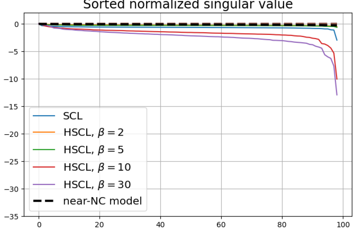
To gain further insights into the DC phenomenon, we trained a model using HSCL with for epochs until it nearly attains NC as measured by the three NC metrics (zero-sum, unit-norm, and equal inner-product) shown in the second row of Table 2. We call this representation mapping (or pre-trained model) the “near-NC” representation mapping (pre-trained model).
Next, with the near-NC representation mapping as initialization, we continue to train the model for an additional 400 epochs under 10 different settings corresponding to hard supervised and hard unsupervised contrastive learning with different hardness levels. Rows 3-12 in Table 2 show the final values of the three NC metrics for the 10 settings. The resulting normalized singular value plots are shown in the second row of Fig. 4.
| Setting | Zero-sum | Unit-norm | Equal inner-product |
| near-NC model | 0.012 | 0.004 | |
| SCL | 0.006 | 0.007 | |
| HSCL, | 0.005 | 0.004 | |
| HSCL, | 0.007 | 0.002 | |
| HSCL, | 0.007 | 0.002 | |
| HSCL, | 0.004 | 0.001 | |
| UCL | 0.005 | 0.005 | |
| HUCL, | 0.005 | 0.003 | |
| HUCL, | 0.004 | 0.002 | |
| HUCL, | 0.093 | 0.047 | |
| HUCL, | 0.761 | 0.586 |
From Table 2 we note that in all supervised settings, the final representation mappings have NC metrics that are very similar to those of initial near-NC mapping. However, in the unsupervised settings, especially HUCL for , the unit-norm and equal inner-product metrics of the final representation mappings are significantly larger than those of the initial near-NC mapping. This shows that mini-batch Adam optimization of CL losses exhibit dynamics that are different in the supervised and unsupervised settings and are impacted by the hardness level of the negative samples.
From the second row of Fig. 4 we make the following observations:
-
•
SCL and HSCL trained with near-NC initialization and Adam do not exhibit DC or DC is negligible (second row and first column of Fig. 4).
-
•
UCL trained with near-NC initialization and Adam also does not exhibit DC, but the behavior of HUCL depends on the hardness level . A larger value appears to make DC more pronounced. This could be explained by the fact that a higher value increases the odds of latent-class collision.

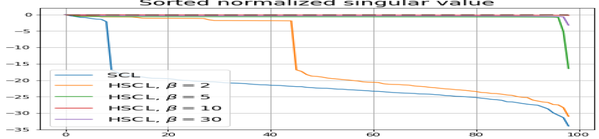
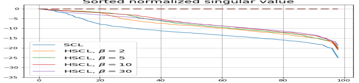
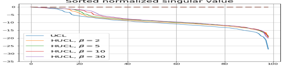
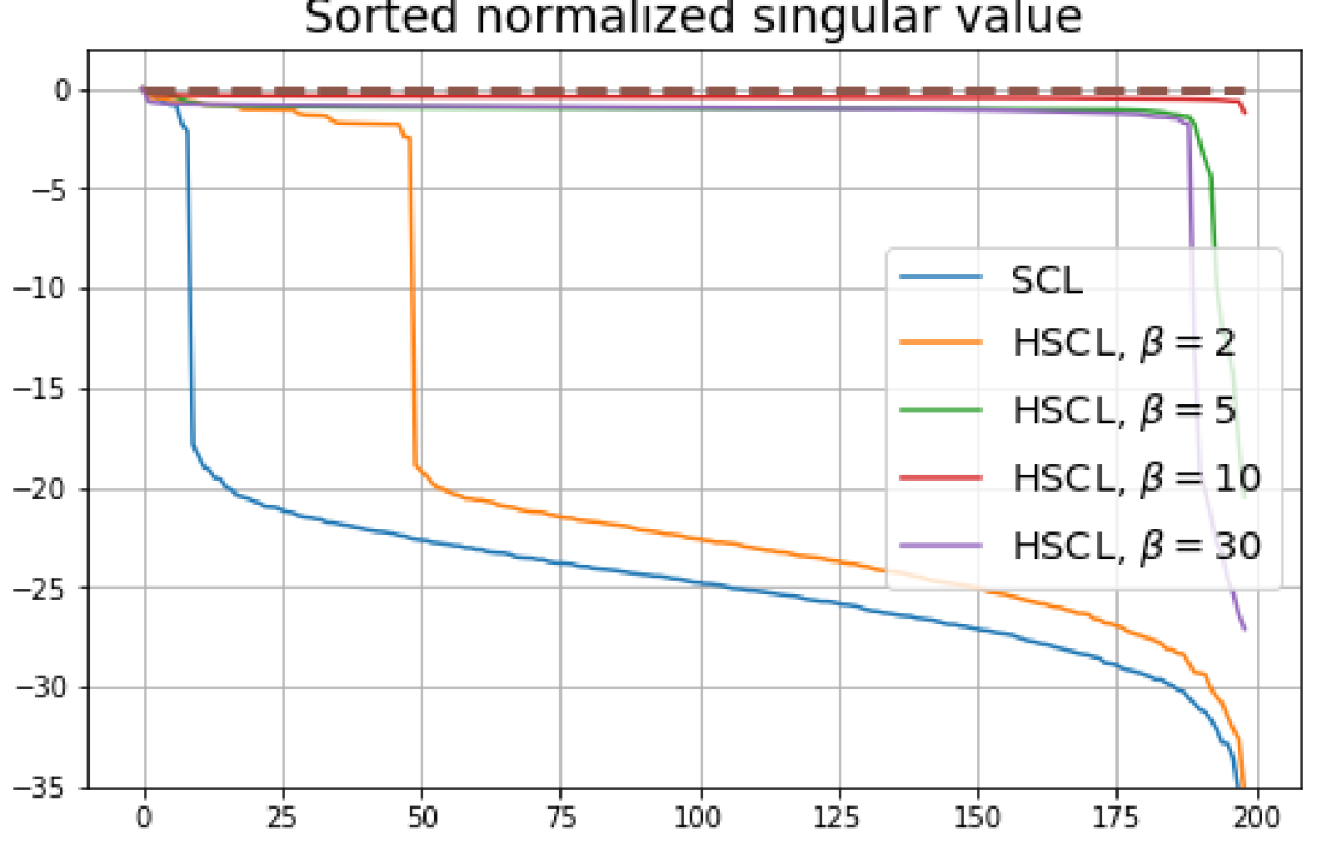
5.5 Role of normalization
Feature normalization also plays an important role in alleviating DC. To demonstrate this, we test three normalization conditions during training: (1) unit-ball normalization, (2) unit-sphere normalization, and (3) no normalization. The resulting normalized singular value plots are shown in Fig. 4 (rows 1, 3, and 4). As can be observed, the behavior of unit-sphere normalization is close to that of unit-ball normalization, and with hard-negative sampling, both SCL and UCL can achieve NC (for suitable hardness levels). Without normalization, neither random-negative nor hard-negative training methods attain NC and they suffer from DC. We also observe that for SCL and UCL, absence of normalization leads to less DC (compare blue curves in rows 1 and 4 of Fig. 4). However, feature normalization could potentially reduce DC in hard-negative sampling for a range of hardness levels.
5.6 Impact of batch size
In Appendix B.3, we report results using different batch sizes. We observe that when the batch size is decreased to 64, NC is still evident in HSCL and HUCL for certain values of . However, when the batch size is further reduced to 32, NC is no longer observed.
5.7 Role of hardening function
5.8 Experiments using the SimCLR framework
In Appendix B.5 we report results using the state-of-the-art SimCLR framework for contrastive learning which uses augmentations to generate samples. The results of Figs. 12 and 13 in Appendix B.5 are somewhat similar to those in Figs. 3 and 4, respectively, but a key difference is the failure to attain NC in the SimCLR sampling framework for both supervised and unsupervised settings at all hardness levels. This is primarily because the SimCLR sampling framework does not utilize label information and cannot guarantee property in Theorem 2 and Theorem 3 nor (for UCL) the conditional independence of anchor and positive samples given their label.
6 Conclusion and open questions
We proved the theoretical optimality of the NC-geometry for SCL, UCL, and notably (for the first time) HSCL losses for a very general family of CL losses and hardening functions that subsume popular choices. We empirically demonstrated the ability of hard-negative sampling to achieve global optima for CL and mitigate dimension collapse, in both supervised and unsupervised settings. Our theoretical and empirical results motivate a number of open questions. Firstly, a tight lower bound for HUCL remains open due to latent-class collision. It is also unclear whether the HUCL loss is minimized iff there is Neural-Collapse. Our theoretical results for the SCL setting did not require conditional independence of anchor and positive samples given their label, but our results for the UCL setting did. A theoretical characterization of the geometry of optimal solutions for UCL in the absence of conditional independence remains open. A difficulty with empirically observing NC in UCL and HUCL is that the number of latent classes is not known because it is, in general, implicitly tied to the properties of the sampling distribution requiring one to choose a sufficiently large representation dimension. Another open question is to unravel precisely how and why hard-negatives alter the optimization landscape enabling the training dynamics of Adam with random initialization to converge to the global optimum for suitable hardness levels and what are optimum hardness levels.
7 Acknowledgements
This research was supported by NSF 1931978.
Appendix A Compatibility of sampling model with SimCLR-like augmentations
The following generative model captures the manner in which many data augmentation mechanisms, including SimCLR, generate a pair of anchor and positive samples. First, a label is sampled. The label may represent an observed class in the supervised setting or a latent (implicit, unobserved) cluster index in the unsupervised setting. Then given , a reference sample is sampled with conditional distribution . Then a pair of samples are generated given via two independent calls to an augmentation mechanism whose behavior can be statistically described by a conditional probability distribution , i.e., . Finally, the representations and are computed via a mapping , e.g., a neural network. Under the setting just described, it follows that both and have identical conditional distributions given which we denote by . This can be verified by checking that both and have the same conditional distribution given equal to
where the integrals will be sums in the discrete (probability mass function) setting. Note that although are conditionally IID given , they need not be conditionally IID given just .
Appendix B Additional experiments
We replicated the same experiments conducted in Sec. 5 on CIFAR10. The results are plotted in Fig. 5 and Fig. 6. In contrast to CIFAR10 and CIFAR100 where the numerical results are provided under three different settings, namely, unit-ball normalization with random initialization, unit-ball normalization with Neural-Collapse initialization, and unit-sphere normalization with random initialization, for Tiny-ImageNet, we only conduct experiments under unit-ball normalization with random initialization. This is because the size of the Tiny-ImageNet dataset (120000 images) is much larger than the sizes of both CIFAR10 and CIFAR100 datasets (50000 images per dataset) which results in a significantly longer processing time. The results for Tiny-ImageNet are plotted in Fig. 7.
B.1 Neural-Collapse and Dimensional-Collapse
For CIFAR10, from Fig. 5 and Fig. 6, we observe similar phenomena as those for CIFAR100. As before, we note that while Theorems 2 and 3 suggest that Neural-Collapse should occur in both the supervised and unsupervised settings when using the random negative sampling method, one may not be able to observe Neural-Collapse in unsupervised settings in practice. For the supervised case in CIFAR10, any degree of hardness propels the representation towards Neural-Collapse. This may be due to the small number of classes in CIFAR10.
For Tiny-ImageNet, from Fig. 7, we observe that when , the geometry of the learned representation closely aligns with that of Neural-Collapse. However, in HUCL, a high degree of hardness can be harmful. At , the geometry most closely approximates Neural-Collapse for both CIFAR10 and Tiny-ImageNet. However, increasing the degree of hardness further, for example at , causes the center of class means to deviate from the origin and the equal inner-product condition is heavily violated.
Furthermore, from the the normalized singular values for CIFAR10 in Fig. 6 and for Tiny-ImageNet in Fig. 7, we observe that random negative sampling without any hardening () suffers from DC whereas hard-negative sampling consistently mitigates DC. The supervised case benefits more from a higher degree of hardness, since in the unsupervised cases there are higher chances of (latent) class collisions.
B.2 Effects of initialization and normalization
The normalized singular value plots for CIFAR10 are shown in Fig. 6. Compared to CIFAR 100 (see Fig. 4), the phenomenon of DC in CIFAR10 is far less pronounced. This may be because CIFAR10 has a smaller number of classes compared to CIFAR100 (10 vs. 100). However, the effects of initialization and normalization on the learned representation geometry are similar to that for CIFAR100:
Effects of initialization: 1) SCL and HSCL trained with near-NC initialization and Adam do not exhibit DC and 2) UCL trained with near-NC initialization and Adam also does not exhibit DC, but the behavior of HUCL depends on the hardness level .
Effects of normalization: The behavior of unit-sphere normalization is close to that of unit-ball normalization, and with hard-negative sampling (and suitable hardness levels), both SCL and UCL can achieve NC. Without normalization, neither regular nor hard-negative training methods attain NC and they suffer from DC. We also observe that with random-negative sampling, un-normalized representations lead to reduced DC in both SCL and UCL. However, hard-negative sampling benefits more from feature normalization and its absence leads to more severe DC.
B.3 Experiments with different batch sizes
To investigate the effect of batch size on the outcomes, we conducted experiments with varying batch sizes. All previous experiments were performed with a batch size of 512. In this section, we present results for batch sizes of 64 and 32 in Fig. 8 and Fig. 9, respectively.
We observe that when the batch size is reduced to 64, Neural-Collapse is still nearly achieved in both HSCL () and HUCL (). However, with a further reduction of batch size to 32, Neural-Collapse is only achieved in HSCL (), and it fails to occur in HUCL for any value of .
B.4 Experiments with a different hardening function
To explore whether similar results can be achieved with a different hardening function, we investigated the impact that changing the hardening function has on NC and DC under unit-ball normalization. We conducted experiments using the CIFAR10 and CIFAR100 datasets adopting the setup consistent with previous experiments but used a new family of hardening functions having the following polynomial form: , for the following set of hardness values . We note that this family of hardening functions decays at a significantly slower rate compared to the exponential hardening function we used in all our previous experiments.
Results for CIFAR100 and CIFAR10 are plotted in Figs. 10 and 11, respectively. We observe phenomena similar to those in Figs. 3 and 5. By selecting an appropriate hardening parameter , we can achieve, or nearly achieve, NC in both supervised and unsupervised settings. Consequently, we can draw conclusions that are qualitatively similar to those in Sec. B.1. Specifically, hard-negative sampling in both supervised and unsupervised settings can mitigate DC while achieving NC.
B.5 Experiments with the SimCLR framework
We conducted additional experiments using the state-of-the-art SimCLR framework for Contrastive Learning. Instead of sampling positive samples from the same class directly, we follow the setting in SimCLR which uses two independent augmentations of a reference sample to create the positive pair. No label information is used to generate the anchor-positive pair.
Figure 12 shows results for SimCLR sampling using the loss function proposed in SimCLR which is the large- asymptotic form of the InfoNCE loss:
| (42) |
where is a weighting hyper-parameter that is set to batch size minus two. Compared to our previous experiments, all the NC metrics deviate significantly away from zero in both supervised and unsupervised settings and all hardness levels. Still, the high-level conclusions for DC are qualitatively similar to those from our previous experiments, specifically that hard-negative sampling can mitigate DC in both supervised and unsupervised settings.
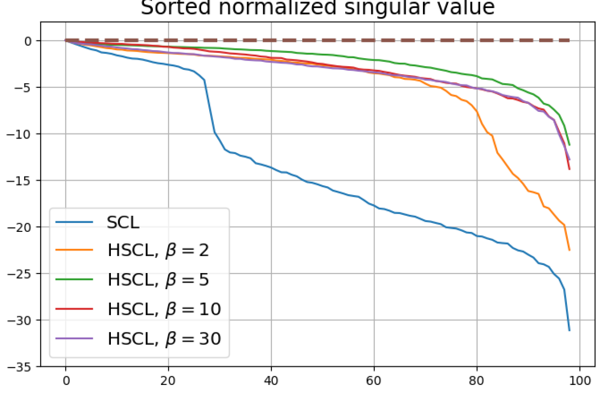
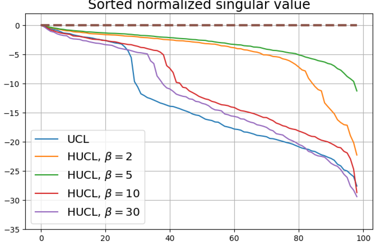
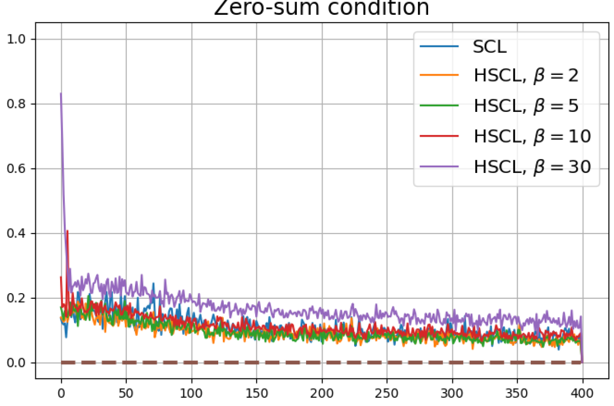
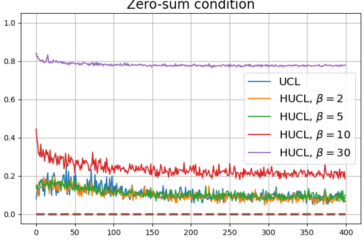
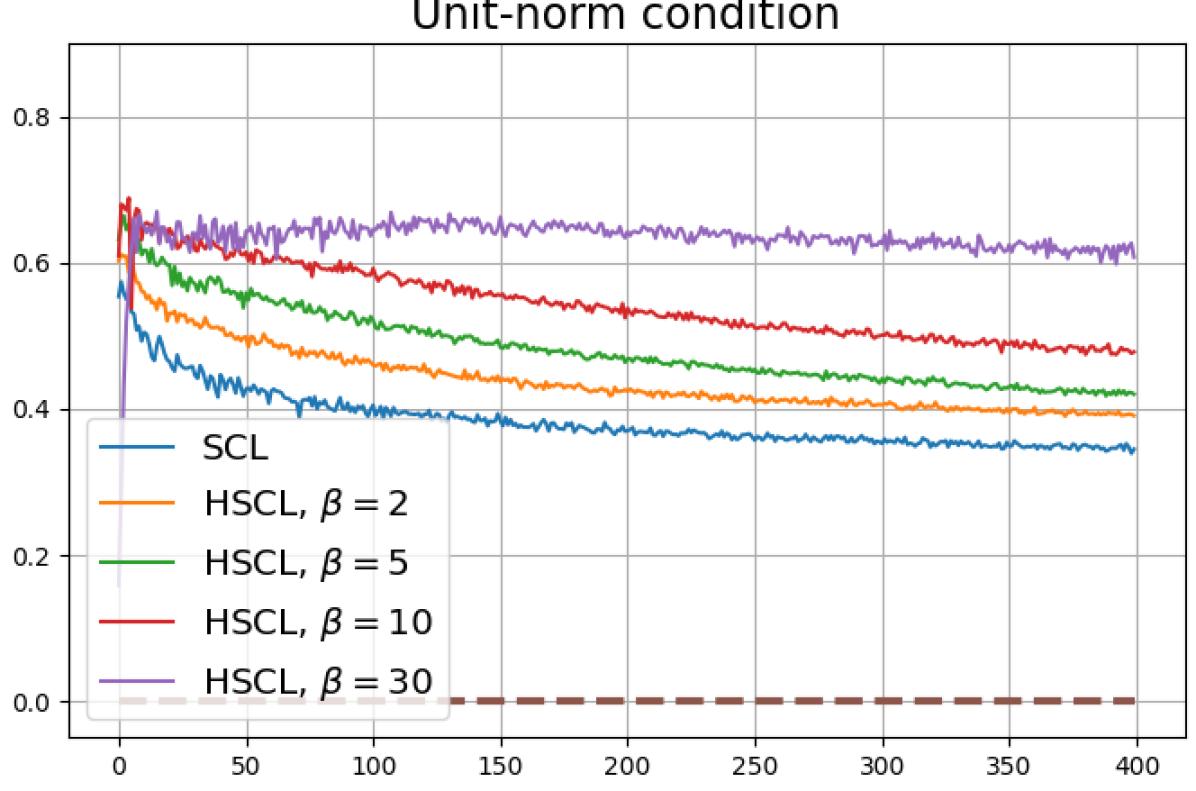
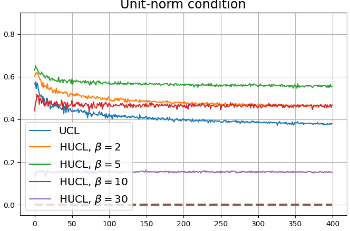
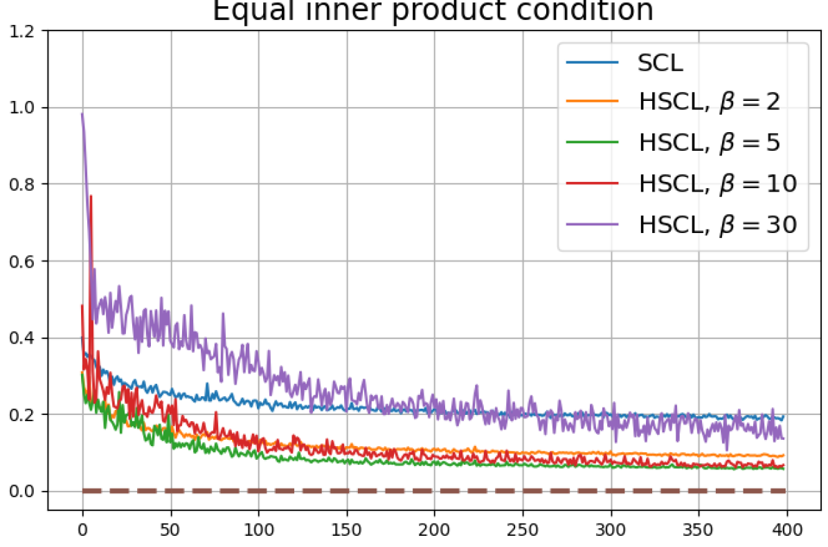
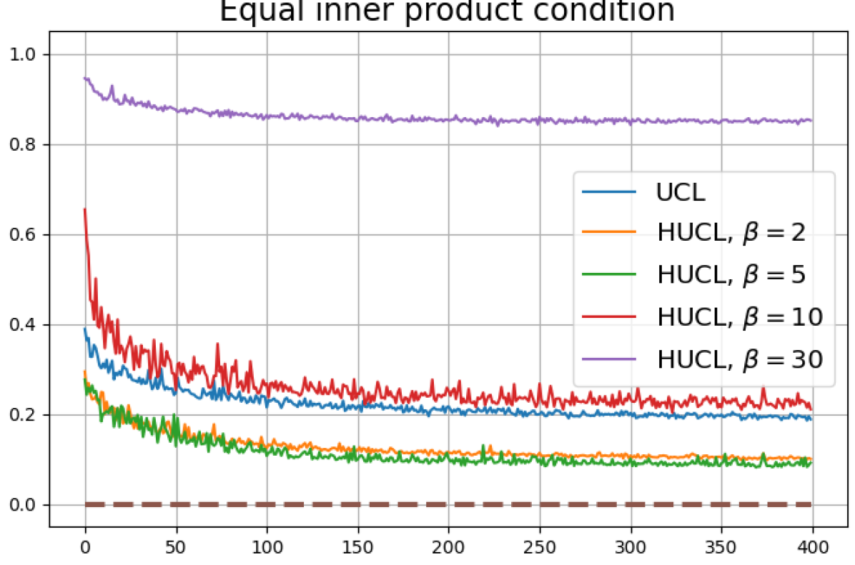
Figure 13 shows results for SimCLR sampling using the InfoNCE loss with and a positive distribution that only relies on the augmentation method. The results are very similar to those in Fig. 12. Since the results in Figs. 12 and 13 share the same SimCLR sampling framework but different losses, it follows that the failure to attain NC is not due to the particular loss function used, but the SimCLR sampling framework itself which does not utilize label information to generate samples. From the unit-norm metric plots in both figures it is clear that the final representations are mostly distributed within the unit-ball than on its surface.
Bibliography
- [1] Sanjeev Arora, Hrishikesh Khandeparkar, Mikhail Khodak, Orestis Plevrakis, and Nikunj Saunshi. A theoretical analysis of contrastive unsupervised representation learning. arXiv preprint arXiv:1902.09229, 2019.
- [2] Randall Balestriero, Mark Ibrahim, Vlad Sobal, Ari Morcos, Shashank Shekhar, Tom Goldstein, Florian Bordes, Adrien Bardes, Gregoire Mialon, Yuandong Tian, et al. A cookbook of self-supervised learning. arXiv preprint arXiv:2304.12210, 2023.
- [3] Stéphane Boucheron, Gábor Lugosi, and Pascal Massart. Concentration Inequalities - A Nonasymptotic Theory of Independence. Oxford University Press, 2013.
- [4] Ting Chen, Simon Kornblith, Mohammad Norouzi, and Geoffrey Hinton. A simple framework for contrastive learning of visual representations. In International conference on machine learning, pages 1597–1607. PMLR, 2020.
- [5] Ching-Yao Chuang, Joshua Robinson, Yen-Chen Lin, Antonio Torralba, and Stefanie Jegelka. Debiased contrastive learning. Advances in neural information processing systems, 33:8765–8775, 2020.
- [6] Patrick Feeney and Michael C Hughes. Sincere: Supervised information noise-contrastive estimation revisited. arXiv preprint arXiv:2309.14277, 2023.
- [7] Florian Graf, Christoph Hofer, Marc Niethammer, and Roland Kwitt. Dissecting supervised contrastive learning. In International Conference on Machine Learning, pages 3821–3830. PMLR, 2021.
- [8] Jeff Z HaoChen, Colin Wei, Adrien Gaidon, and Tengyu Ma. Provable guarantees for self-supervised deep learning with spectral contrastive loss. Advances in Neural Information Processing Systems, 34:5000–5011, 2021.
- [9] Kaiming He, Xiangyu Zhang, Shaoqing Ren, and Jian Sun. Deep residual learning for image recognition. In 2016 IEEE Conference on Computer Vision and Pattern Recognition (CVPR), pages 770–778, 2016.
- [10] Ruijie Jiang, Prakash Ishwar, and Shuchin Aeron. Hard negative sampling via regularized optimal transport for contrastive representation learning. In 2023 International Joint Conference on Neural Networks (IJCNN), pages 1–8. IEEE, 2023.
- [11] Ruijie Jiang, Thuan Nguyen, Prakash Ishwar, and Shuchin Aeron. Supervised contrastive learning with hard negative samples. arXiv preprint arXiv:2209.00078, 2022.
- [12] Li Jing, Pascal Vincent, Yann LeCun, and Yuandong Tian. Understanding dimensional collapse in contrastive self-supervised learning. In International Conference on Learning Representations, 2021.
- [13] Prannay Khosla, Piotr Teterwak, Chen Wang, Aaron Sarna, Yonglong Tian, Phillip Isola, Aaron Maschinot, Ce Liu, and Dilip Krishnan. Supervised contrastive learning. Advances in Neural Information Processing Systems, 33:18661–18673, 2020.
- [14] Alex Krizhevsky, Geoffrey Hinton, et al. Learning multiple layers of features from tiny images. 2009.
- [15] Ya Le and Xuan Yang. Tiny imagenet visual recognition challenge. CS 231N, 7(7):3, 2015.
- [16] Jason D Lee, Qi Lei, Nikunj Saunshi, and Jiacheng Zhuo. Predicting what you already know helps: Provable self-supervised learning. Advances in Neural Information Processing Systems, 34:309–323, 2021.
- [17] Zijun Long, George Killick, Richard McCreadie, Gerardo Aragon Camarasa, and Zaiqiao Meng. When hard negative sampling meets supervised contrastive learning, 2023.
- [18] Vassili Nikolaevich Malozemov and Aleksandr Borisovich Pevnyi. Equiangular tight frames. Journal of Mathematical Sciences, 157(6):789–815, 2009.
- [19] Hyun Oh Song, Yu Xiang, Stefanie Jegelka, and Silvio Savarese. Deep metric learning via lifted structured feature embedding. In Proceedings of the IEEE conference on computer vision and pattern recognition, pages 4004–4012, 2016.
- [20] Aaron van den Oord, Yazhe Li, and Oriol Vinyals. Representation learning with contrastive predictive coding. arXiv preprint arXiv:1807.03748, 2018.
- [21] Vardan Papyan, XY Han, and David L Donoho. Prevalence of neural collapse during the terminal phase of deep learning training. Proceedings of the National Academy of Sciences, 117(40):24652–24663, 2020.
- [22] Advait Parulekar, Liam Collins, Karthikeyan Shanmugam, Aryan Mokhtari, and Sanjay Shakkottai. Infonce loss provably learns cluster-preserving representations. arXiv preprint arXiv:2302.07920, 2023.
- [23] Nils Rethmeier and Isabelle Augenstein. A primer on contrastive pretraining in language processing: Methods, lessons learned, and perspectives. ACM Computing Surveys, 55(10):1–17, 2023.
- [24] Joshua David Robinson, Ching-Yao Chuang, Suvrit Sra, and Stefanie Jegelka. Contrastive learning with hard negative samples. In International Conference on Learning Representations, 2020.
- [25] Joshua David Robinson, Ching-Yao Chuang, Suvrit Sra, and Stefanie Jegelka. Contrastive learning with hard negative samples. In International Conference on Learning Representations, 2021.
- [26] Nguyen Thuan, Jiang Ruijie, Aeron Shuchin, Ishwar Prakash, and Brown Donald. On neural collapse in contrastive learning with imbalanced datasets. In IEEE International Workshop on Machine Learning for Signal Processing, 2024.
- [27] Tongzhou Wang and Phillip Isola. Understanding contrastive representation learning through alignment and uniformity on the hypersphere. In International Conference on Machine Learning, pages 9929–9939. PMLR, 2020.
- [28] Yifei Wang, Qi Zhang, Yisen Wang, Jiansheng Yang, and Zhouchen Lin. Chaos is a ladder: A new theoretical understanding of contrastive learning via augmentation overlap. In International Conference on Learning Representations, 2021.
- [29] Zixin Wen and Yuanzhi Li. Toward understanding the feature learning process of self-supervised contrastive learning. In International Conference on Machine Learning, pages 11112–11122. PMLR, 2021.
- [30] Mike Wu, Milan Mosse, Chengxu Zhuang, Daniel Yamins, and Noah Goodman. Conditional negative sampling for contrastive learning of visual representations. arXiv preprint arXiv:2010.02037, 2020.
- [31] Zhirong Wu, Yuanjun Xiong, Stella X Yu, and Dahua Lin. Unsupervised feature learning via non-parametric instance discrimination. In Proceedings of the IEEE conference on computer vision and pattern recognition, pages 3733–3742, 2018.
- [32] Can Yaras, Peng Wang, Zhihui Zhu, Laura Balzano, and Qing Qu. Neural collapse with normalized features: A geometric analysis over the riemannian manifold. Advances in neural information processing systems, 35:11547–11560, 2022.
- [33] Jinxin Zhou, Xiao Li, Tianyu Ding, Chong You, Qing Qu, and Zhihui Zhu. On the optimization landscape of neural collapse under mse loss: Global optimality with unconstrained features. In International Conference on Machine Learning, pages 27179–27202. PMLR, 2022.
- [34] Liu Ziyin, Ekdeep Singh Lubana, Masahito Ueda, and Hidenori Tanaka. What shapes the loss landscape of self supervised learning? In The Eleventh International Conference on Learning Representations, 2022.