HAT-P-7b: An Extremely Hot Massive Planet Transiting a Bright Star in the Kepler Field
Abstract
We report on the latest discovery of the HATNet project; a very hot giant planet orbiting a bright () star with a small semi-major axis of AU. Ephemeris for the system is days, mid-transit time (BJD). Based on the available spectroscopic data on the host star and photometry of the system, the planet has a mass of and radius of . The parent star is a slightly evolved F6 star with , , K, and metallicity . The relatively hot and large host star, combined with the close orbit of the planet, yield a very high planetary irradiance of erg cm-2 s-1, which places the planet near the top of the pM class of irradiated planets as defined by Fortney et al. (2007). If as predicted by Fortney et al. (2007) the planet re-radiates its absorbed energy before distributing it to the night side, the day-side temperature should be about K. Because the host star is quite bright, measurement of the secondary eclipse should be feasible for ground-based telescopes, providing a good opportunity to compare the predictions of current hot Jupiter atmospheric models with the observations. Moreover, the host star falls in the field of the upcoming Kepler mission; hence extensive space-borne follow-up, including not only primary transit and secondary eclipse observations but also asteroseismology, will be possible.
Subject headings:
planetary systems — stars: individual (HAT-P-7, GSC 03547-01402) techniques: spectroscopic1. Introduction
Transiting planets provide unique information about the nature and evolution of extrasolar planets because they yield direct measurement of the radius and (together with radial velocity data) mass of these objects. Many of these planets are found in quite close-in orbits of their parent stars, in which case the radiation from the parent star may be expected to play a major role in controlling the structure and dynamics of their atmospheres. Transiting planets with very tight orbits about their parent stars are heated sufficiently that their thermal emission is measurable, both at times of secondary eclipse and for some, throughout their orbit (see e.g. Deming et al., 2005; Knutson et al., 2007; Harrington et al., 2007). Such observations, together with observations in different spectral bands of the depth and shape of primary transits, open up the possibility of detailed understanding of the composition, structure, and dynamics of “hot Jupiter” atmospheres. (See e.g. Fortney et al. (2007), Hubeny et al. (2003), Burrows et al. (2006).
Here we report on the HATNet project’s detection of a very hot Jupiter that transits a bright, F6 star, with a day period and semi-major axis of only AU. The parent star (hereafter denoted HAT-P-7), with K and radius has such a high luminosity as to make the surface temperature of this very close-orbiting planet among the highest of any known transiting planet.
Because HAT-P-7 is relatively bright, this opens up the possibility of a number of interesting follow-on studies from space and ground. Notably, the host star is also in the field of view of the forthcoming Kepler mission. This means that many transits will very likely be recorded with extremely high photometric precision during the operational phase of Kepler starting in 2009. Timing variations in the transits, if detected, could indicate the presence of other bodies in the system, such as terrestrial-mass planets or Trojan satellites. For this reason, preparatory observations of transits and secondary eclipses in the HAT-P-7 system undertaken in advance of the mission could significantly increase the scientific return from later observations of the star by Kepler.
The next section (§ 2) describes the photometric detection of the HAT-P-7b planet by the HATNet monitoring system; § 3 outlines both the photometric and spectroscopic follow-up observations; § 4 explains our analysis of these data including derivation of stellar and planetary parameters as well as verification that the signal derives from a transiting planet rather than a “false-positive”; and finally, § 5 discusses the results and implications for further studies of this intriguing system.
2. Photometric detection
The HATNet telescopes HAT-7 and HAT-8 (HATNet; Bakos et al., 2002, 2004) observed HATNet field G154, centered at , , on a near-nightly basis from 2004 May 27 to 2004 August 6. Exposures of 5 minutes were obtained at a 5.5-minute cadence whenever conditions permitted; all in all 5140 exposures were secured, each yielding photometric measurements for approximately stars in the field down to . The field was observed in network mode, exploiting the longitude separation between HAT-7, stationed at the Smithsonian Astrophysical Observatory’s (SAO) Fred Lawrence Whipple Observatory (FLWO) in Arizona (W), and HAT-8, installed on the rooftop of SAO’s Submillimeter Array (SMA) building atop Mauna Kea, Hawaii (W). We note that each light curve obtained by a given instrument was shifted to have a median value to be the same as catalogue magnitude of the appropriate star, allowing to merge light curves acquired by different stations and/or detectors.
Following standard frame calibration procedures, astrometry was performed as described in Pál & Bakos (2006), and aperture photometry results were subjected to External Parameter Decorrelation (EPD, described briefly in Bakos et al., 2007), and also to the Trend Filtering Algorithm (TFA; Kovács et al., 2005). We searched the light curves of field G154 for box-shaped transit signals using the BLS algorithm of Kovács et al. (2002). A very significant periodic dip in brightness was detected in the magnitude star GSC 03547-01402 (also known as 2MASS 19285935+4758102; , ; J2000), with a depth of mmag, a period of days and a relative duration (first to last contact) of , equivalent to a duration of hours.
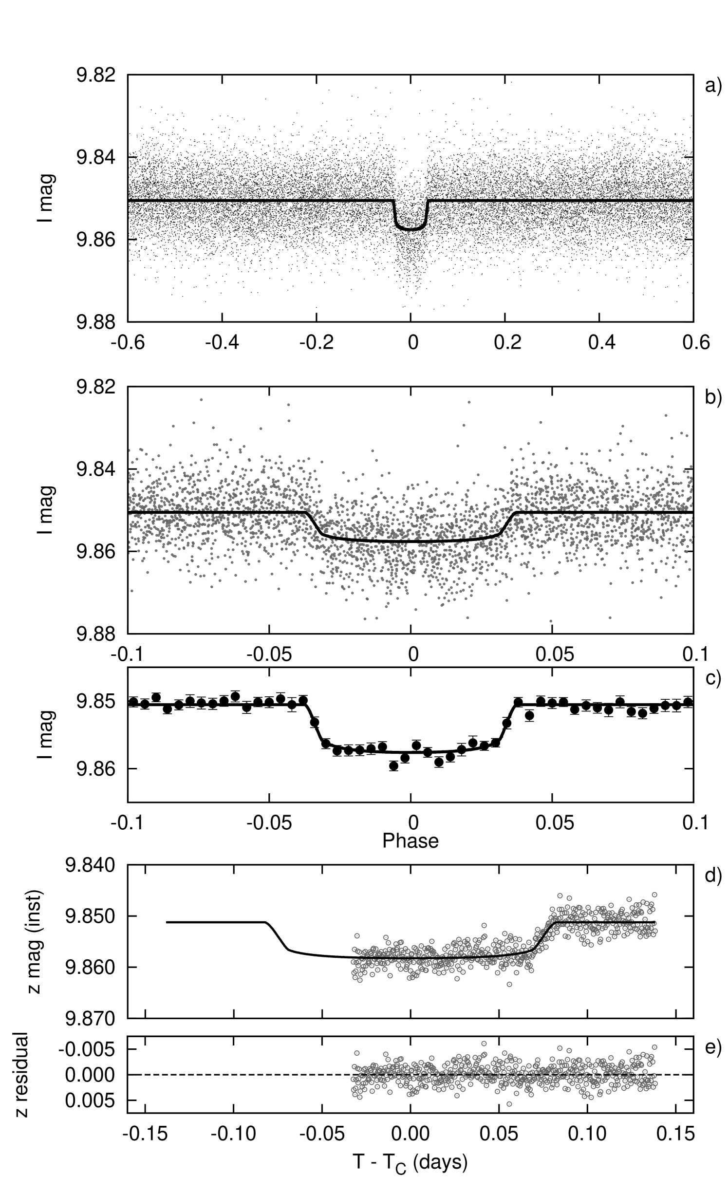
In addition, the star happened to fall in the overlapping area between fields G154 and G155. Field G155, centered at , , was also observed over an extended time in between 2004 July 27 and 2005 September 20 by the HAT-6 (Arizona) and HAT-9 (Hawaii) telescopes. We gathered 1220 and 10260 data-points, respectively (which independently confirmed the transit), yielding a total number of 16620 data-points. The combined HATNet light curve after the EPD and TFA procedures is plotted on Figs. 1a,b, superimposed on these plots is our best fit model (see § 4). We note that TFA was run in signal reconstruction mode, i.e. systematics were iteratively filtered out from the observed time series assuming that the underlying signal is a trapeze-shaped transit (see Kovács et al., 2005, for additional details).
In addition to having a significant overlap with each other, we note that fields G154 and G155 both intersect the field of view of the upcoming Kepler mission (Borucki et al., 2007).
3. Follow-up observations
3.1. Low-resolution Spectroscopy
Following the HATNet photometric detection, HAT-P-7 (then a transit candidate) was observed spectroscopically with the CfA Digital Speedometer (DS, see Latham, 1992) at the FLWO 1.5 m Tillinghast reflector, in order to rule out a number of blend scenarios that mimic planetary transits (e.g. Brown, 2003; O’Donovan et al., 2007), as well as to characterize the stellar parameters, such as surface gravity, effective temperature, and rotation. Four spectra were obtained over an interval of 29 days. These observations cover Å in a single echelle order centered at Å, and have a resolving power of . Radial velocities were derived by cross-correlation, and have a typical precision of . Using these measurements, we have ruled out an unblended companion of stellar mass (e.g. an M dwarf orbiting an F dwarf), since the radial velocities did not show any variation within the uncertainties. The mean heliocentric radial velocity of HAT-P-7 was measured to be . Based on an analysis similar to that described in Torres et al. (2002), the DS spectra indicated that the host star is a slightly evolved dwarf with (cgs), K and .
3.2. High resolution spectroscopy
For the characterization of the radial velocity variations and for the more precise determination of the stellar parameters, we obtained 8 exposures with an iodine cell, plus one iodine-free template, using the HIRES instrument (Vogt et al., 1994) on the Keck I telescope, Hawaii, between 2007 August 24 and 2007 September 1. The width of the spectrometer slit was resulting a resolving power of , while the wavelength coverage was Å. The iodine gas absorption cell was used to superimpose a dense forest of lines on the stellar spectrum and establish an accurate wavelength fiducial (see Marcy & Butler, 1992). Relative radial velocities in the Solar System barycentric frame were derived as described by Butler et al. (1996), incorporating full modeling of the spatial and temporal variations of the instrumental profile. The final radial velocity data and their errors are listed in Table 1. The folded data, with our best fit (see § 4.2) superimposed, are plotted in Fig. 2a.
3.3. Photometric follow-up observations
Partial photometric coverage of a transit event of HAT-P-7 was carried out in the Sloan -band with the KeplerCam CCD on the 1.2 m telescope at FLWO, on 2007 November 2. The total number of frames taken from HAT-P-7 was 514 with cadence of 28 seconds. During the reduction of the KeplerCam data, we used the following method. After bias and flat calibration of the images, an astrometric transformation (in the form of first order polynomials) between the brightest stars and the 2MASS catalog was derived, as described in Pál & Bakos (2006), yielding a residual of pixel. Aperture photometry was then performed using a series of apertures of with the radius of 4, 6 and 8 pixels in fixed positions calculated from this solution and the actual 2MASS positions. The instrumental magnitude transformation was obtained using stars on a frame taken near culmination of the field. The transformation fit was initially weighted by the estimated photon- and background-noise error of each star, then the procedure was repeated weighting by the inverse variance of the light curves. From the set of apertures we have chosen the aperture for which the out-of-transit (OOT) rms of HAT-P-7 was the smallest; the radius of this aperture is 6 pixels. This light curve was then de-correlated against trends using the OOT sections, which yielded a light curve with an overall rms of 1.9mmag at a cadence of one frame per 28 seconds. This is a bit larger than the expected rms of 1.5mmag, derived from the photon noise (1.2mmag) and scintillation noise – which has an expected amplitude of 0.8mmag, based on the observational conditions and the calculations of Young (1967) – possibly due to unresolved trends and other noise sources. The resulting light curve is shown in Fig. 1d.
4. Analysis
The analysis of the available data was done in five steps. First, an independent analysis was performed on the HATNet, the radial velocity (RV) and the high precision photometric follow-up (FU) data, respectively. Analysis of the HATNet data yielded an initial value for the orbital period and transit epoch. The initial period and epoch were used to fold the RV’s, and phase them with respect to the predicted transit time for a circular orbit. The HATNet and the RV epochs together yield a more accurate period, since the time difference between the discovery light curve and the RV follow-up is fairly long; more than 3 years. Using this refined period, we can extrapolate to the expected center of the KeplerCam partial transit, and therefore obtain a fit for the two remaining key parameters describing the light curve: where is the semi-major axis for a circular orbit, and the impact parameter , where is the inclination of the orbit.
Second, using as starting points the initial values as derived above, we performed a joint fit of the HATNet, RV and FU data, i.e. fitting all of the parameters simultaneously. The reason for such a joint fit is that the three separate data-sets and the fitted parameters are intertwined. For example, the epoch (depending partly on the RV fit) has a relatively large error, affecting the extrapolation of the transit center to the KeplerCam follow-up.
In all of the above procedures, we used the downhill simplex method to search for the best fit values and the method of refitting to synthetic data sets to find out the error of the adjusted parameters. The latter method yields a Monte-Carlo set of the a posteriori distribution of the fit parameters.
The third step of the analysis was the derivation of the stellar parameters, based on the spectroscopic analysis of the host star (high resolution spectroscopy using Keck/HIRES), and the physical modeling of the stellar evolution, based on existing isochrone models. As the fourth step, we then combined the results of the joint fit and stellar parameter determination to determine the planetary and orbital parameters of the HAT-P-7b system. Finally, we have done a blend analysis to confirm that the orbiting companion is a hot Jupiter. In the following subsections we give a detailed description of the above main steps of the analysis.
| BJD | RV | ||
|---|---|---|---|
| (2,454,000) | () | () | |
| 336.73958 . | |||
| 336.85366 . | |||
| 337.76211 . | |||
| 338.77439 . | |||
| 338.85455 . | |||
| 339.89886 . | |||
| 343.83180 . | |||
| 344.98804 . |
4.1. Independent fits
For the independent fit procedure, we first analyzed the HATNet light curves, as observed by the HAT-6, HAT-7, HAT-8 and HAT-9 telescopes. Using the initial period and transit length from the BLS analysis, we fitted a model to the 214 cycles of observations spanned by all the HATNet data. Although at this stage we were interested only in the epoch and period, we have used the transit light curve model with the assumption quadratic limb darkening, where the flux decrease was calculated using the models provided by Mandel & Agol (2002). In principle, fitting the epoch and period as two independent variables is equivalent to fitting the time instant of the centers of the first and last observed individual transits, and , with a constraint that all intermediate transits are regularly spaced with period . Note that this fit takes into account all transits that occurred during the HATNet observations, even though it is described only by and . The fit yielded (BJD) and (BJD). The period derived from the and epochs was days. Using these values, we found that there were 326 cycles between and the end of the RV campaign. The epoch extrapolated to the approximate time of RV measurements was (BJD). Note that the error in is much smaller than the period itself ( days), so there is no ambiguity in the number of elapsed cycles when folding the periodic signal.
We then analyzed the radial velocity data in the following way. We defined the transit as that being closest to the end of the radial velocity measurements. This means that the first transit observed by HATNet (at ) was the event. Given the short period, we assumed that the orbit has been circularized (Hut, 1981) (later verified; see below). The orbital fit is linear if we choose the radial velocity zero-point and the amplitudes and as adjusted values, namely:
| (1) |
where is an arbitrary time instant (chosen to be BJD), is the semi-amplitude of the RV variations, and is the initial period taken from the previous independent HATNet fit. The actual epoch can be derived from the above equation since for circular orbits transit center occurs when the RV curve has the most negative slope. Using the equations above, we derived the initial epoch of the transit center to be (BJD). We also performed a more general (non-linear) fit to the RV in which we let the eccentricity float. This fit yielded an eccentricity consistent with zero, namely and . Therefore, we adopt a circular orbit in the further analysis.
Combining the RV epoch with the first epoch observed by HATNet (), we obtained a somewhat refined period, days. This was fed back into phasing the RV data, and we performed the RV fit again to the parameters , and . The fit yielded , and (BJD). This epoch was used to further refine the period to get d, where the error calculation assumes that and are uncorrelated. At this point we stopped the above iterative procedure of refining the epoch and period; instead a final refinement of epoch and period was obtained through performing a joint fit, (as described later in § 4.2). We note that in order to get a reduced chi-square value near unity for the radial velocity fit, it was necessary to quadratically increase the noise component with an amplitude of , which is well within the range of stellar jitter observed for late F stars; see Butler et al. (2006).
Using the improved period and the epoch , we extrapolated to the center of KeplerCam follow-up transit (). Since the follow-up observation only recorded a partial event (see Fig. 1d), this extrapolation was necessary to improve the light curve modeling. For this, we have used a quadratic limb-darkening approximation, based on the formalism of Mandel & Agol (2002). The limb-darkening coefficients were based on the results of the SME analysis (notably, ; see § 4.3 for further details), which yielded and . Using these values and the extrapolated time of the transit center, we adjusted the light curve parameters: the relative radius of the planet , the square of the impact parameter and the quantity as independent parameters (see Bakos et al., 2007, for the choice of parameters). The result of the fit was , and day-1, where the uncertainty of the transit center time due to the relatively high error in the transit epoch was also taken into account in the error estimates.

4.2. Joint fit
The results of the individual fits described above provide the starting values for a joint fit, i.e. a simultaneous fit to all of the available HATNet, radial velocity and the partial follow-up light curve data. The adjusted parameters were , the time of first transit center in the HATNet campaign, , the out-of-transit magnitude of the HATNet light curve in -band and the previously defined parameters of , , , , and . We note that in this joint fit all of the transits in the HATNet light curve have been adjusted simultaneously, tied together by the constraint of assuming a strictly periodic signal; the shape of all these transits were characterized by , and (and the limb-darkening coefficients) while the distinct transit center time instants were interpolated using and , via the RV fit. For initial values we used the results of the independent fits (§ 4.1). The error estimation based on method refitting to synthetic data sets gives the distribution of the adjusted values, and moreover, this distribution can be used directly as an input for a Monte-Carlo parameter determination for stellar evolution modeling, as described later (§ 4.3).
Final results of the joint fit were: (BJD), mag, , , , , and . Using the distribution of these parameters, it is straightforward to obtain the values and the errors of the additional parameters derived from the joint derived fit, namely , , and . All final fit parameters are listed in Table 3.
| Parameter | Value | Source |
|---|---|---|
| (K). | SMEaaSME = ‘Spectroscopy Made Easy’ package for analysis of high-resolution spectra Valenti & Piskunov (1996). See text. | |
| . | SME | |
| (). | SME | |
| (). | Y2+LC+SMEbbY2+LC+SME = Yale-Yonsei isochrones (Yi et al., 2001), light curve parameters, and SME results. | |
| (). | Y2+LC+SME | |
| (cgs). | Y2+LC+SME | |
| (). | Y2+LC+SME | |
| (mag). | Y2+LC+SME | |
| Age (Gyr). | Y2+LC+SME | |
| Distance (pc). | Y2+LC+SME |
4.3. Stellar parameters
The results of the joint fit enable us to refine the parameters of the star. First, the iodine-free template spectrum from Keck was used for an initial determination of the atmospheric parameters. Spectral synthesis modeling was carried out using the SME software (Valenti & Piskunov, 1996), with wavelength ranges and atomic line data as described by Valenti & Fischer (2005). We obtained the following initial values: effective temperature K, surface gravity (cgs), iron abundance , and projected rotational velocity . The rotational velocity is slightly smaller than the value given by the DS measurements. The temperature and surface gravity correspond to a slightly evolved F6 star. The uncertainties quoted here and in the remaining of this discussion are twice the statistical uncertainties for the values given by the SME analysis. This reflects our attempt, based on prior experience, to incorporate systematic errors (e.g. Noyes et al. (2008); see also Valenti & Fischer (2005)). Note that the previously discussed limb darkening coefficients, , , and have been taken from the tables of Claret (2004) by interpolation to the above-mentioned SME values for , , and .
As described by Sozzetti et al. (2007), is a better luminosity indicator than the spectroscopic value of since the variation of stellar surface gravity has a subtle effect on the line profiles. Therefore, we used the values of and from the initial SME analysis, together with the distribution of to estimate the stellar properties from comparison with the Yonsei-Yale (Y2) stellar evolution models by Yi et al. (2001). Since a Monte-Carlo set for values has been derived during the joint fit, we performed the stellar parameter determination as follows. For a selected value of , two Gaussian random values were drawn for and with the mean and standard deviation as given by SME (with formal SME uncertainties doubled as indicated above).Using these three values, we searched the nearest isochrone and the corresponding mass by using the interpolator provided by Demarque et al. (2004). Repeating this procedure for values of , , , the set of the a posteriori distribution of the stellar parameters was obtained, including the mass, radius, age, luminosity and color (in multiple bands). The age determined in this way is Gy with a statistical uncertainty of Gy; however, the uncertainty in the theoretical isochrone ages is about 1.0 Gy. Since the corresponding value for the surface gravity of the star, (cgs),is well within 1- of the value determined by the SME analysis, we accept the values from the joint fit as the final stellar parameters. These parameters are summarized in Table 2.
We note that the Yonsei-Yale isochrones contain the absolute magnitudes and colors for different photometric bands from up to , providing an easy comparison of the estimated and the observed colors. Using these data, we determined the and colors of the best fitted stellar model: and . Since the colors for the infrared bands provided by Yi et al. (2001) and Demarque et al. (2004) are given in the ESO photometric standard system, for the comparison with catalog data, we converted the infrared color to the 2MASS system using the transformations given by Carpenter (2001). The color of the best fit stellar model was , which is in fairly good agreement with the actual 2MASS color of HAT-P-7: . We have also compared the color of the best fit model to the catalog data, and found that although HAT-P-7 has a low galactic latitude, , the model color agrees well with the observed TASS color of (see Droege et al., 2006). Hence, the star is not affected by the interstellar reddening within the errors, since . For estimating the distance of HAT-P-7, we used the absolute magnitude (resulting from the isochrone analysis, see also Table 2) and the observed magnitude. These two yield a distance modulus of , i.e. distance of pc.
4.4. Planetary and orbital parameters
The determination of the stellar properties was followed by the characterization of the planet itself. Since Monte-Carlo distributions were derived for both the light curve and the stellar parameters, the final planetary and orbital data were also obtained by the statistical analysis of the a posteriori distribution of the appropriate combination of these two Monte-Carlo data sets. We found that the mass of the planet is , the radius is and its density is . We note that in the case of binary systems with large mass and radius ratios (such as the one here) there is a strong correlation between and (see e.g. Beatty et al., 2007). This correlation is also exhibited here with . The final planetary parameters are also summarized at the bottom of Table 3.
Due to the way we derived the period, i.e. , one can expect a large correlation between the epochs , and the period itself. Indeed, and , while the correlation between the two epochs is negligible; . It is easy to show that if the signs of the correlations between two epochs and (in our case and ) and the period are different, respectively, then there exists an optimal epoch , which has the smallest error among all of the interpolated epochs. We note that will be such that it also exhibits the smallest correlation with the period. If and are the respective uncorrelated errors of the two epochs, then
| (2) |
where square brackets denote the time of the transit event nearest to the time instance . In the case of HAT-P-7b, and , the corresponding epoch is the event at (BJD). The final ephemeris and planetary parameters are summarized in Table 3.
| Parameter | Value |
|---|---|
| Light curve parameters | |
| (days) . | |
| () . | |
| (days)aa: total transit duration, time between first to last contact; : ingress/egress time, time between first and second, or third and fourth contact. . | |
| (days)aa: total transit duration, time between first to last contact; : ingress/egress time, time between first and second, or third and fourth contact. . | |
| . | |
| . | |
| . | |
| (deg) . | |
| Spectroscopic parameters | |
| () . | |
| () . | |
| . | (adopted) |
| Planetary parameters | |
| () . | |
| () . | |
| . | |
| () . | |
| (AU) . | |
| (cgs) . | |
4.5. Excluding blend scenarios
Following Torres et al. (2007), we explored the possibility that the measured radial velocities are not real, but instead caused by distortions in the spectral line profiles due to contamination from a nearby unresolved eclipsing binary. In that case the “bisector span” of the average spectral line should vary periodically with amplitude and phase similar to the measured velocities themselves (Queloz et al., 2001; Mandushev et al., 2005). We cross-correlated each Keck spectrum against a synthetic template matching the properties of the star (i.e. based on the SME results, see § 4.3), and averaged the correlation functions over all orders blueward of the region affected by the iodine lines. From this representation of the average spectral line profile we computed the mean bisectors, and as a measure of the line asymmetry we computed the “bisector spans” as the velocity difference between points selected near the top and bottom of the mean bisectors (Torres et al., 2005). If the velocities were the result of a blend with an eclipsing binary, we would expect the line bisectors to vary in phase with the photometric period with an amplitude similar to that of the velocities. Instead, we detect no variation in excess of the measurement uncertainties (see Fig. 2c). We have also tested the significance of the correlation between the radial velocity and the bisector variations. Therefore, we conclude that the velocity variations are real and that the star is orbited by a Jovian planet. We note here that the mean bisector span ratio relative to the radial velocity amplitude is the smallest () among all the HATNet planets, indicating an exceptionally high confidence that the RV signal is not due to a blend with an eclipsing binary companion.
5. Discussion
With orbital period of only 2.2 days, implying a semi-major axis of only AU, HAT-P-7b, is a “very hot Jupiter”, a name frequently given to giant planets with orbital period less than 3 days (see Bouchy et al., 2004). However, what really matters is the incident flux from the parent star, which for HAT-P-7b is exceptionally high because (a) the large radius of the parent star ( ) combined with the small semi-major axis yields a very small geometrical factor (whose inverse describes the stellar flux impinging on the planet); and (b) its parent star has relatively high effective temperature: K. The flux impinging on the planet is erg cm-2s-1. This places it among the most highly irradiated members of the “pM” class of planets, as discussed by Fortney et al. (2007).
For a pM class planet, Fortney et al. (2007) argue that the incident radiation is absorbed by TiO and VO molecules in a hot stratosphere, and almost immediately re-radiated, rather than being partially advected to the night side of the planet, as would be the case if the radiation were absorbed deeper down in the cooler atmosphere of a “pL” planet, which would not have gaseous TiO and VO in its atmosphere.
For a pM planet, the dayside temperature would be given by
| (3) |
where is the Bond albedo, which we assume to be essentially zero (see, e.g. Rowe et al., 2007), and the redistribution factor (see Lopez-Morales and Seager, 2007). For HAT-P-7 this yields a dayside temperature of K. If at the other extreme, contrary to the theory of Fortney et al. (2007), the incident energy absorbed by HAT-P-7b were to be distributed isotropically over the planet’s surface before being re-emitted, as is predicted for “pL” planets too cool to have significant TiO and VO in their atmospheres, then in Equation 3, and the day-side temperature would be K. Thus, detection and measurement of the emission from the dayside of HAT-P-7b would yield an important test of the theory of Fortney et al. (2007).
Lopez-Morales and Seager (2007) and Fortney et al. (2007) noted that the thermal emission in the optical and near infrared from very hot Jupiters should be detectable from the ground. Lopez-Morales and Seager (2007) identified OGLE-TR-56b, the only other known very hot jupiter with predicted dayside temperature as high as that of HAT-P-7b, as a particularly promising candidates. However, since HAT-P-7 is 6 magnitudes brighter than OGLE-TR-56, it is a far better candidate for secondary eclipse studies from the ground. For HAT-P-7, the brightness decrease in -band at secondary eclipse should be or in the respective cases of zero (pM-type) or complete (pL-type) planet-wide re-distribution of irradiated stellar flux. This implies that in the former case the eclipse could be detected at the 2-sigma level with a 1.2-m telescope with a -band integration of 4 hours during eclipse (that is, the total eclipse duration), plus 4 more hours of out-of-eclipse observation. We plan to carry out such observations in the near future with the KeplerCam on FLWO 1.2 m and with MMT 6.5 m (also at FLWO) telescopes.
Recently Pollacco et al. (2007) reported the discovery of the transiting exoplanet WASP-3b, located 0.0317 AU from an F star with K and radius ; this indicates a very high radiative flux at the planet of erg cm-2s-1, comparable to but about 25% smaller than the radiative flux at HAT-P-7b. For the same reasons as for the case of HAT-P-7b discussed above, this almost certainly will be a pM-class planet, so that its dayside temperature should be about 2530K, as indicated by Equation 3 with and . This planet should also be detectable in visible or near infrared radiation. In fact, if it is a pM planet, the depth of secondary eclipse as seen in -band should be similar to that for HAT-P-7b, namely : although with its lower dayside temperature the surface brightness of WASP-3b should be smaller than for HAT-P-7b, the geometrical factor is larger, because WASP-3 is a less evolved star.
HAT-P-7b has an additional important property in that it is in the field of view of one of the detectors on the forthcoming Kepler mission (Borucki et al., 2007), currently scheduled for launch in early 2009 to monitor stars for photometric signals from transiting planets and other forms of stellar variability. Hence, HAT-P-7 should be subjected to intense and regular photometric observations for several years starting in 2009. This will permit extremely high precision light curves of the primary transit, the secondary transit, and perhaps also the variation of thermal and reflected light emission from the planet over the course of its orbit as described above. In addition, it will be possible to search intensively for transit timing variations over the several year lifetime of the mission. Such observations could yield important information about orbital variations due to other companions in the system including terrestrial-mass or smaller planets or Trojans, or to other effects such as precession of the orbital plane or the orbital line of nodes. To maximize the scientific return from Kepler in this regard, it would be very useful to obtain high precision light curves both from the ground, and from space instruments such as Epoxi and MOST, in the very near term for later comparison with Kepler observations.
Asteroseismology of HAT-P-7 using Kepler could yield an independent measurement of the star’s mean density from the “large separation” between p-modes of the same low angular degree (e.g. Stello et al., 2007). This would provide a check on the mean density of the star completely independent of that derived from the transit measurements of the parameter. Equivalently, the asteroseismology measurements would yield an independent measurement of the stellar radius, and hence a more precise value for the radius of the planet HAT-P-7b. Such a rich combined data set could have additional benefits for understanding stellar structure and evolution.
References
- Bakos et al. (2002) Bakos, G. Á., Lázár, J., Papp, I., Sári, P. & Green, E. M. 2002, PASP, 114, 974
- Bakos et al. (2004) Bakos, G. Á., Noyes, R. W., Kovács, G., Stanek, K. Z., Sasselov, D. D., & Domsa, I. 2004, PASP, 116, 266
- Bakos et al. (2007) Bakos, G. Á., et al. 2007a, ApJ, 670, 826
- Bakos et al. (2007) Bakos, G. Á., et al. 2007b, ApJ, 671, 173
- Beatty et al. (2007) Beatty, T. G. et al. 2007, ApJ, 663, 573
- Borucki et al. (2007) Borucki, W. J. et al. 2006, ASP Conf. Ser., 366, 309
- Bouchy et al. (2004) Bouchy, F. et al. 2007, A&A, 421, 13
- Brown (2003) Brown, T. M. 2003, ApJ, 593, L125
- Burrows et al. (2006) Burrows, A., Sudarsky, D., and Hubeny, I. 2006, ApJ, 650, 1140
- Butler et al. (1996) Butler, R. P. et al. 1996, PASP, 108, 500
- Butler et al. (2006) Butler, R. P., Wright, J., Marcy, G., Fischer, D., Vogt, S., Tinney, C., Jones, H., Carter, B., Johnson, J, McCarthy, C. Penny, A. 2006, ApJ, 646, 505
- Carpenter (2001) Carpenter, J. 2001, AJ, 121, 2851
- Claret (2004) Claret, A. 2004, A&A, 428, 1001
- Demarque et al. (2004) Demarque et al. 2004, ApJ, 155, 667
- Deming et al. (2005) Deming, D., Seager, S., Richardson, L. J., Harrington, J. 2005, Nature, 434, 740
- Droege et al. (2006) Droege, T. F., Richmond, M. W., & Sallman, M. 2006, PASP, 118, 1666
- Fortney et al. (2007) Fortney, J. J., Lodders, K., Marley, M., Freedman, R. 2007, astroph/0710.2558
- Gaudi (2005) Gaudi, B. S., Seager, S., Mallen-Ornelas, G. 2005, ApJ, 623, 472
- Harrington et al. (2007) Harrington, J., Luszcz, S., Seager, S., Deming, D., & Richardson, L. J. 2007, Nature, 447, 691
- Hubeny et al. (2003) Hubeney, I., Burrows, A., Sudarsky, D. 2003, ApJ, 594, 1011
- Hut (1981) Hut, P. 1981, A&A, 99, 126
- Knutson et al. (2007) Knutson, H. A., et al. 2007, Nature, 447, 183
- Kovács et al. (2002) Kovács, G., Zucker, S., & Mazeh, T. 2002, A&A, 391, 369
- Kovács et al. (2005) Kovács, G., Bakos, G. Á., & Noyes, R. W. 2005, MNRAS, 356, 557
- Latham (1992) Latham, D. W. 1992, in IAU Coll. 135, Complementary Approaches to Double and Multiple Star Research, ASP Conf. Ser. 32, eds. H. A. McAlister & W. I. Hartkopf (San Francisco: ASP), 110
- Lopez-Morales and Seager (2007) Lopez-Morales, M. & Seager, S. 2007, in press (astroph/0708.0822)
- Mandel & Agol (2002) Mandel, K., & Agol, E. 2002, ApJ, 580, L171
- Mandushev et al. (2005) Mandushev, G. et al. 2005, ApJ, 621, 1061
- Marcy & Butler (1992) Marcy, G. W., & Butler, R. P. 1992, PASP, 104, 270
- Noyes et al. (2008) Noyes, R. W. et al. 2008, ApJ, 673, L79
- Ochsenbein et al. (2000) Ochsenbein, F., Bauer, P., & Marcout, J. 2000, A&AS, 143, 23
- O’Donovan et al. (2007) O’Donovan, F. T. et al. 2007, ApJ, 662, 658
- Pál & Bakos (2006) Pál, A., & Bakos, G. Á. 2006, PASP, 118, 1474
- Pollacco et al. (2007) Pollacco, D. et al. 2007, MNRAS, submitted (astroph/0711.0126)
- Queloz et al. (2001) Queloz, D. et al. 2001, A&A, 379, 279
- Rowe et al. (2007) Rowe, J. et al. 2007, in press (astroph/0711.4111)
- Sozzetti et al. (2007) Sozzetti, A. et al. 2007, ApJ, 664, 1190
- Stello et al. (2007) Stello, D., Kjeldsen, H. &, Bedding, T. R. 2007, PASP, in press (astroph/0702051)
- Torres et al. (2002) Torres, G., Boden, A. F., Latham, D. W., Pan, M. & Stefanik, R. P. 2002, AJ, 124, 1716
- Torres et al. (2005) Torres, G., Konacki, M., Sasselov, D. D., & Jha, S. 2005, ApJ, 619, 558
- Torres et al. (2007) Torres, G. et al. 2007, ApJ, 666, 121
- Torres, Winn & Holman (2008) Torres, G., Winn, J. N., Holman, M. J. 2008, ApJ, in press (astroph/0801.1841)
- Valenti & Fischer (2005) Valenti, J. A., & Fischer, D. A. 2005, ApJS, 159, 141
- Valenti & Piskunov (1996) Valenti, J. A., & Piskunov, N. 1996, A&AS, 118, 595
- Vogt et al. (1994) Vogt, S. S. et al. 1994, Proc. SPIE, 2198, 362
- Yi et al. (2001) Yi, S. K. et al. 2001, ApJS, 136, 417
- Young (1967) Young, A. T. 1967, AJ, 72, 747