HDPView: Differentially Private Materialized View for Exploring High Dimensional Relational Data
Abstract.
How can we explore the unknown properties of high-dimensional sensitive relational data while preserving privacy? We study how to construct an explorable privacy-preserving materialized view under differential privacy. No existing state-of-the-art methods simultaneously satisfy the following essential properties in data exploration: workload independence, analytical reliability (i.e., providing error bound for each search query), applicability to high-dimensional data, and space efficiency. To solve the above issues, we propose HDPView, which creates a differentially private materialized view by well-designed recursive bisected partitioning on an original data cube, i.e., count tensor. Our method searches for block partitioning to minimize the error for the counting query, in addition to randomizing the convergence, by choosing the effective cutting points in a differentially private way, resulting in a less noisy and compact view. Furthermore, we ensure formal privacy guarantee and analytical reliability by providing the error bound for arbitrary counting queries on the materialized views. HDPView has the following desirable properties: (a) Workload independence, (b) Analytical reliability, (c) Noise resistance on high-dimensional data, (d) Space efficiency. To demonstrate the above properties and the suitability for data exploration, we conduct extensive experiments with eight types of range counting queries on eight real datasets. HDPView outperforms the state-of-the-art methods in these evaluations.
PVLDB Reference Format:
PVLDB, 15(9): 1766 - 1778, 2022.
doi:10.14778/3538598.3538601
††This work is licensed under the Creative Commons BY-NC-ND 4.0 International License. Visit https://creativecommons.org/licenses/by-nc-nd/4.0/ to view a copy of this license. For any use beyond those covered by this license, obtain permission by emailing info@vldb.org. Copyright is held by the owner/author(s). Publication rights licensed to the VLDB Endowment.
Proceedings of the VLDB Endowment, Vol. 15, No. 9 ISSN 2150-8097.
doi:10.14778/3538598.3538601
1. Introduction
In the early stage of data science workflows, exploring a database to understand its properties in terms of multiple attributes is essential to designing the subsequent tasks. To understand the properties, data analysts need to issue a wide variety of range counting queries. If the database is highly sensitive (e.g., personal healthcare records), data analysts may have little freedom to explore the data due to privacy issues (Su et al., 2020; Wang et al., 2019).
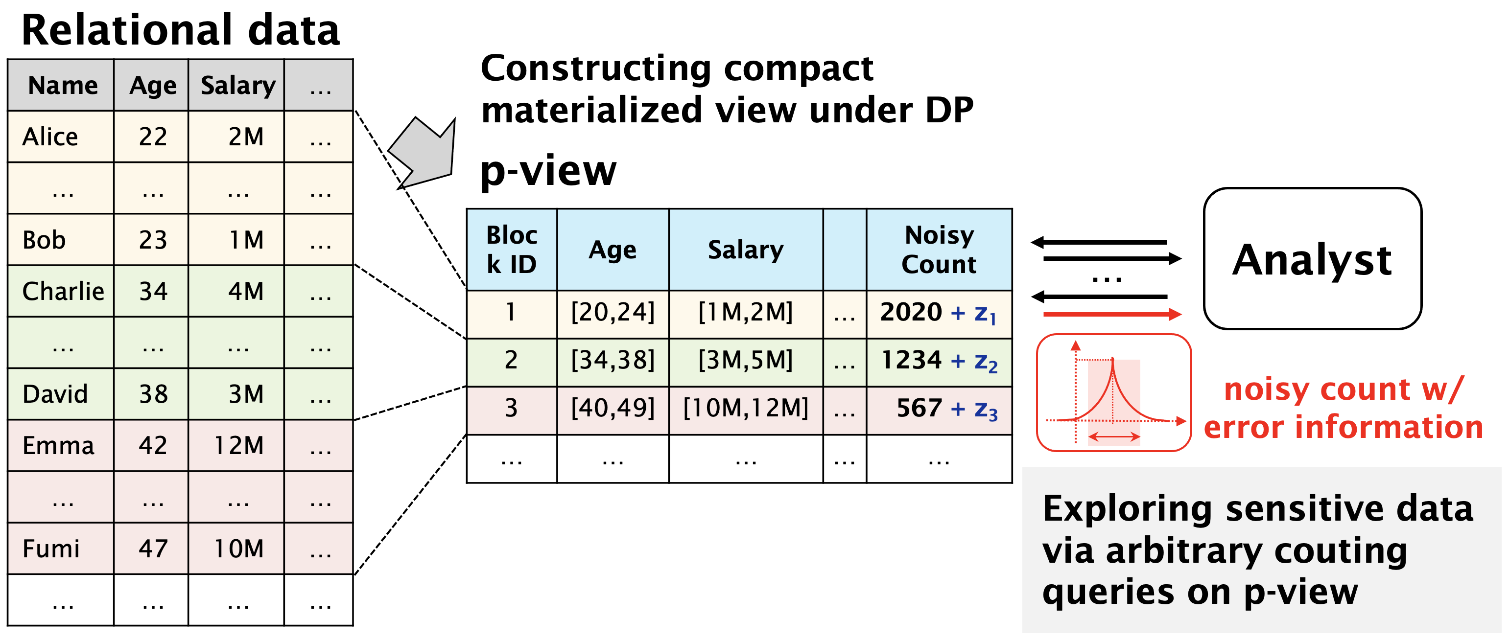
How can we explore the properties of high-dimensional sensitive data while preserving privacy? This paper focuses on guaranteeing differential privacy (DP) (Dwork, 2006; Dwork et al., 2014) via random noise injections. As Figure 1 shows, we especially study how to construct a privacy-preserving materialized view (p-view for short) of relational data, which enables data analysts to explore arbitrary range counting queries in a differential private way. Note that once a p-view is created, the privacy budget is not consumed any more for publishing counting queries, different from interactive differentially private query systems (Johnson et al., 2018a; Ge et al., 2019; Wilson et al., 2019; Rogers et al., 2020; Johnson et al., 2018b), which consume the budget every time queries are issued. In this work, we describe the desirable properties of the p-view, especially in data exploration for high-dimensional data, and fill the gaps of the existing methods.
| Identity111Identity adds noise to the entries of the count vector by the Laplace mechanism (Dwork, 2006) and cannot directly perturb high-dimensional datasets due to the domains being too large; we measure estimated error using the method described in (McKenna et al., 2018). (Dwork, 2006) | Privtree (Zhang et al., 2016) | HDMM (McKenna et al., 2018) | PrivBayes (Zhang et al., 2017) | HDPView (ours) | |
|---|---|---|---|---|---|
| Workload independence | ✓ | ✓ | ✓ | ✓ | |
| Analytical reliability | ✓ | ✓ | ✓ | ✓ | |
| Noise resistance on high-dimensional | only low-dimensional | ✓ | ✓ | ✓ | |
| Space efficiency | ✓ | ✓ | ✓ |
Several methods for constructing a p-view have been studied in the existing literature. The most primitive method is to add Laplace noise (Dwork, 2006) to each cell of the count tensor (or vector) representing the original histogram and publish the perturbed data as a p-view. While this noisy view can answer arbitrary range counting queries with a DP guarantee, it accumulates a large amount of noise. Data-aware partitioning methods (Li et al., 2014; Zhang et al., 2014; Qardaji et al., 2013; Xiao et al., 2012; Yaroslavtsev et al., 2013; Zhang et al., 2016; Kotsogiannis et al., 2019) are potential solutions, but they focus only on low-dimensional data due to the high complexity of discovering the optimal partitioning when the data have multiple attributes. Additionally, these methods require exponentially large spaces as the dimensionality of the data increases due to the count tensor representation, which can easily make them impractical. Workload-aware optimization methods (Li et al., 2014, 2015; McKenna et al., 2018; Kotsogiannis et al., 2019) are promising techniques for releasing query answers for high-dimensional data; however, they cannot provide query-independent p-views needed in data exploration.
In addition, one of the most popular approaches these days is differentially private learning of generative models (Qardaji et al., 2014; Chen et al., 2015; Zhang et al., 2017; Jordon et al., 2018; Takagi et al., 2021; Harder et al., 2021; Fan et al., 2020; Zhang et al., 2021; Ge et al., 2020). Through the training of deep generative models (Jordon et al., 2018; Takagi et al., 2021; Harder et al., 2021; Ge et al., 2020; Fan et al., 2020) or graphical models (Zhang et al., 2017, 2021), counting queries and/or marginal queries can be answered directly from the model or indirectly with synthesized data via sampling. These methods are very space efficient because the synthetic dataset or graphical model can be used to answer arbitrary counting queries. However, these families rely on complex optimization methods such as DP-SGD (Abadi et al., 2016), and it is very difficult to quantitatively estimate the error of counting queries using synthetic data, which eventually leads to a lack of reliability in practical use. Unlike datasets often used in the literature, the data collected in the practical field may be completely unmodelable. Table 1 summarizes a comparison between the most related works and our method, HDPView, i.e., High-Dimensional Private materialized View. Each method is described in more detail in Section 2.
Our target use case is privacy-preserving data exploration on high-dimensional data, for which the p-view should have the following four properties:
-
•
Workload independence: Data analysts desire to issue arbitrary queries for exploring data. These queries should not be predefined.
-
•
Analytical reliability: For reliability in practical data exploration, it is necessary to be able to estimate the scale of the error for arbitrary counting queries.
-
•
Noise resistance on high-dimensional data: Range counting queries compute the sum over the range and accumulate the noise injected for DP. This noise accumulation makes the query answers useless. To avoid this issue, we need a robust mechanism even for high-dimensional data.
-
•
Space efficiency: It is necessary to generate spatially efficient views even for count tensors with a large number of total domains on various datasets.
Our proposal. To satisfy all the above requirements, we propose a simple yet effective recursive bisection method on a high-dimensional count tensor, HDPView. Our proposed method has the same principle as (Xiao et al., 2012; Li et al., 2014; Zhang et al., 2016) of first partitioning a database into small blocks and then averaging over each block with noise. Unlike the existing methods, HDPView can efficiently perform error-minimizing partitioning even on multidimensional count tensors instead of conventional 1D count vectors. HDPView recursively partitions multidimensional blocks at a cutting point chosen in a differentially private manner while aiming to minimize the sum of aggregation error (AE) and perturbation error (PE). Compared to Privtree (Zhang et al., 2016), our proposed method provides a more data-aware flexible cutting strategy and proper convergence of block partitioning, which results in smaller errors in private counting queries and much better spatial efficiency of the generated p-views. Our method provides a powerful and practical solution for constructing a p-view under the DP constraint. More importantly, the p-view generated by HDPView can work as a query processing system and expose the estimated error bound at runtime for any counting query without further privacy consumption. This error information ensures reliable analysis for data explorers.
| Identity11footnotemark: 1 (Dwork, 2006) | Privtree (Zhang et al., 2016) | HDMM (McKenna et al., 2018) | PrivBayes (Zhang et al., 2017) | HDPView (ours) | |
|---|---|---|---|---|---|
| Average relative RMSE | |||||
| Average relative size of p-view | 5578.27 | N/A | N/A |
Contributions. Our contributions are threefold. First, we design a p-view and formalize the segmentation for a multidimensional count tensor to find an effective p-view as error minimizing optimization problem. P-view can be widely used for data exploration process on multidimensional data and is a differentially private approximation of a multidimensional histogram that can release counting queries with analytical reliability. Second, we propose HDPView described above to find a desirable solution to the optimization problem. Our algorithm is more effective than conventional algorithms due to finding flexible partitions and more efficient due to making appropriate convergence decisions. Third, we conduct extensive experiments, whose source code and dataset are open, and show that HDPView has the following merits. (1) Effectiveness: HDPView demonstrates smaller errors for various range counting queries and outperforms the existing methods (Dwork, 2006; Zhang et al., 2016; Li et al., 2014; McKenna et al., 2018; Zhang et al., 2017) on multi-dimensional real-world datasets. (2) Space efficiency: HDPView generates a much more compact representation of the p-view than the state-of-the-art (i.e., Privtree (Zhang et al., 2016)) in our experiment.
Preview of result. We present a summary previewing of the experimental results. Table 2 shows the average relative root mean squared error against (RMSE) of HDPView in eight types of range counting queries on eight real-world datasets and the average relative size of the p-view generated by the algorithms. With Identity, we obtain a p-view by making each cell of the original count tensor a converged block. HDPView yields the smallest error score on average. This is a desirable property for data explorations. Furthermore, compared to that of Privtree (Zhang et al., 2016), the p-view generated by HDPView is more space efficient.
2. Related Works
In the last decade, several works have proposed differentially private methods for exploring sensitive data. Here, we describe the state-of-the-arts related to our work.
Data-aware partitioning. Data-aware partitioning is a conventional method that aims to directly randomize and expose the entire histogram for all domains (e.g., count vector, count tensor); thereby, it can immediately compose a p-view that answers all counting queries. A naïve approach to constructing a differentially private view is adding Laplace noise (Dwork, 2006) to all values of a count vector; this is called the Identity mechanism. This naïve approach results in prohibitive noise on query answers through the accumulation of noise over the grouped bins used by queries. DAWA (Li et al., 2014) and AHP (Zhang et al., 2014) take data-aware partitioning approaches to reduce the amount of noise. The partitioning-based approaches first split a raw count vector into bins and then craft differentially private aggregates by averaging each bin and injecting a single unit of noise in each bin. However, these approaches work only for very low (e.g., one or two) -dimensional data due to the high complexity of discovering the optimal solution when the data have multiple attributes. DPCube (Xiao et al., 2012) is a two-step multidimensional data-aware partitioning method, but the first step, obtaining an accurate approximate histogram, is difficult on high-dimensional data with small counts in each cell.
Privtree (Zhang et al., 2016) and (Cormode et al., 2012) perform multidimensional data-aware partitioning on count tensors, mainly targeting the spatial decomposition task for spatial data. Unlike our method, this method uses a fixed quadtree as the block partitioning strategy, which leads to an increase in unnecessary block partitioning as the dimensionality increases. As a result, it downgrades the spatial efficiency and incurs larger perturbation noise. In addition, this method aims to partition the blocks such that the count value is below a certain threshold, while our proposed method aims to minimize the AE of the blocks and reduce count query noise.
Optimization of given workloads. Another well-established approach is the optimization for a given workload. Li et al. (Li et al., 2015) introduced a matrix mechanism (MM) that crafts queries and outputs optimized for a given workload. The high-dimensional MM (HDMM) (McKenna et al., 2018) is a workload-aware data processing method extending the MM to be robust against noise for high-dimensional data. PrivateSQL (Kotsogiannis et al., 2019) selects the view to optimize from pregiven workloads. In the data exploration process, it is not practical to assume a predefined workload, and these methods are characterized by a loss of accuracy when optimized for a workload of wide variety of queries.
Private data synthesis. Private data synthesis, which builds a privacy-preserving generative model of sensitive data and generates synthetic records from the model, is also useful for data exploration. Note that synthesized dataset can work as a p-view by itself. PrivBayes (Zhang et al., 2017) can heuristically learn a Bayesian network of data distribution in a differentially private manner. DPPro (Xu et al., 2017), Priview (Qardaji et al., 2014) and PrivSyn (Zhang et al., 2021) represent distribution by approximation with several smaller marginal tables. While these methods provide a partial utility guarantee based on randomized mechanisms such as Laplace mechanisms or random projections, they face difficulties in providing an error bound for arbitrary counting queries on the synthesized data. Differentially private deep generative models have also attracted attention (Acs et al., 2018; Jordon et al., 2018; Takagi et al., 2021; Harder et al., 2021), but most of the works focus on the reconstruction of image datasets. Fan et al. (Fan et al., 2020) studied how to build a good generative model based on generative adversarial nets (GAN) for tabular datasets. Their experimental results showed that the utility of differentially private GAN was lower than that of PrivBayes for tabular data. (Ren et al., 2018) provides a solution for high-dimensional data in a local DP setting.
As mentioned in Section 1, the accuracy of these methods has improved greatly in recent years, but it is difficult to guarantee their utility for analysis using counting queries, and there are large gaps in practice. DPPro (Xu et al., 2017) utilizes a random projection (Johnson and Lindenstrauss, 1984) that preserve L2-distance to the original data in an analyzable form to give a utility guarantee, but this is different from the guarantee for each counting query. CSM (Zheng et al., 2019) gives a utility analysis for queries, however, their analysis ignores the effect of information loss due to compression, which may not be accurate. Also, as shown in their experiments, they apply intense preprocessing to the domain size and do not show the effectiveness for high-dimensional data. Our proposed method provides an end-to-end error analysis for arbitrary counting queries by directly constructing p-views from histograms without any intermediate generative model.
Querying and programming framework. PrivateSQL (Kotsogiannis et al., 2019) is a differentially private relational database system for multirelational tables, where for each table, it applies an existing noise-reducing method such as DAWA. Unlike our method, PrivateSQL needs a given workload to design private views to release. Flex (Johnson et al., 2018a), Google’s work (Wilson et al., 2019) and APEx (Ge et al., 2019) are SQL processing frameworks under DP. They issue queries to the raw data, which can consume an infinite amount of the privacy budgets. Hence, we believe that these DP-query processing engines are not suitable for data exploration tasks where many instances of trial and error may be possible. Our method generates p-view, which can be used as a differentially private query system that allows any number of range counting queries to be issued.
3. Preliminaries
This section introduces essential knowledge for understanding our proposal. We first describe notations this paper uses. Then, we briefly explain DP.
3.1. Notation
Let be the input database with records consisting of an attribute set that has attributes . The domain of an attribute has a finite ordered set of discrete values, and the size of the domain is denoted as . The overall domain size of is , where . In the case where attribute is continuous, we transform the domain into a discrete domain by binning, and in the case where attribute is categorical, we transform it into an ordered domain. Then, can be represented as a range where for all , . For ranges , means the number of value satisfies .
We consider transforming the database into the -mode count tensor , where given ranges , represents the number of records where . We utilize as a count value in ; this corresponds to a cell of the count tensor. We denote a subtensor of as block . is also a -mode count tensor, but its domain in each dimension is smaller than or equal to that of the original count tensor ; i.e., each attribute , of and of satisfy and . We denote the domain size of as .
Last, we denote as a counting query and as a workload. is a set of counting queries, where , and returns the counting query results for count tensor .
3.2. Differential Privacy
DP (Dwork, 2006) is a rigorous mathematical privacy definition that quantitatively evaluates the degree of privacy protection when we publish outputs. DP is used in broad domains and applications (Bindschaedler et al., 2017; Chaudhuri et al., 2019; Papernot et al., 2016). The importance of DP is supported by the fact that the US census announced ’2020 Census results will be protected using “differential privacy”, the new gold standard in data privacy protection’ (Abowd, 2018).
Definition 0 (-differential privacy).
A randomized mechanism satisfies -DP if, for any two inputs such that differs from in at most one record and any subset of outputs , it holds that
We define databases and as neighboring databases.
Practically, we employ a randomized mechanism that ensures DP for a function . The mechanism perturbs the output of to cover ’s sensitivity, which is the maximum degree of change over any pair of datasets and .
Definition 0 (Sensitivity).
The sensitivity of a function for any two neighboring inputs is:
where is a norm function defined in ’s output domain.
When is a histogram, equals 1 (Hay et al., 2009). Based on the sensitivity of , we design the degree of noise to ensure DP. The Laplace mechanism and exponential mechanism are well-known as standard approaches.
The Laplace mechanism can be used for randomizing numerical data. Releasing the histogram is a typical use case of this mechanism.
Definition 0 (Laplace Mechanism).
For function , the Laplace mechanism adds noise as:
| (1) |
where denotes a vector of independent samples from a Laplace distribution with mean 0 and scale .
The exponential mechanism is the random selection algorithm. The selection probability is weighted based on a score in a quality metric for each item.
Definition 0 (Exponential Mechanism).
Let be the quality metric for choosing an item in the database . The exponential mechanism randomly samples from with weighted sampling probability defined as follows:
| (2) |
Quantifying the privacy of differentially private mechanisms is essential for releasing multiple outputs. Sequential composition and parallel composition are standard privacy accounting methods.
Theorem 5 (Sequential Composition (Dwork, 2006)).
Let be mechanisms satisfying -, -DP. Then, a mechanism sequentially applying satisfies ()-DP.
Theorem 6 (Parallel Composition (McSherry, 2009)).
Let be mechanisms satisfying -, -DP. Then, a mechanism applying to the disjoint datasets in parallel satisfies -DP.
4. Problem Formulation
4.1. Segmentation as Optimization

This section describes the foundation of multidimensional data-aware segmentation that seeks a solution for the differentially private view from the input count tensor . Every count is sanitized to satisfy DP. We formulate multidimensional block segmentation as an optimization problem.
Foundation. Given a count tensor , we consider partitioning into blocks . The blocks satisfy where , and . We denote the sum over as and its perturbed output as . We can sample with the Laplace mechanism and craft the -differentially private sum in .
For any count in the block , we have two types of errors: Perturbation Error (PE) and Aggregation Error (AE). Assuming that we replace any count with , the absolute error between and can be computed as
| (3) |
Therefore, the total error over block , namely, the segmentation error (SE), can be given by:
| (4) |
where
| (5) | ||||
| (6) |
Problem. The partitioning makes the PE of each block times smaller than those of the original counts with Laplace noise. Furthermore, we consider the expectation of the SE
| (7) |
Thus, to discover the optimal partition , we need to minimize Eq. (7). The optimization problem is denoted as follows:
| (8) |
Challenges. It is not easy to discover the optimal partition . This problem is an instance of the set partitioning problem (Balas and Padberg, 1976), which is known to be NP-complete, where the objective function is computed by brute-force searching for every combination of candidate blocks. It is hard to solve since the search space is basically a very large scale due to large . Therefore, this paper seeks an efficient heuristic solution with a good balance between utility (i.e., smaller errors) and privacy.
4.2. P-view Definition
Our proposed p-view has a simple structure. The p-view consists of a set of blocks, each of which has a range for each attribute and an appropriately randomized count value, as shown in Figure 1. Formally, we define the p-view as follows.
| (9) |
Thus, each block has this -dimensional domain and the sanitized sum of count values .
In the range counting query processing, a counting query needs to have the range condition . Let the ranges of be , and we calculate the intersection of and the block and add the count value according to the size of the intersection. Hence, the result can be calculated as follows.
| (10) |
The number of intersection calculations is proportional to the number of blocks, and the complexity of the query processing is .
5. Proposed Algorithm
This section introduces our proposed solution. Our solution constructs a p-view of the input relational data while preserving utility and privacy with analytical reliability to estimate errors in the arbitrary counting queries against the p-view (Eq.(10)).
5.1. Overview
Our challenge is to devise a simple yet effective algorithm that enables us to efficiently search a block partitioning with small total errors and DP guarantees. As a realization of the algorithm, we propose HDPView.
Figure 2 illustrates an overview of our proposed algorithm. First, HDPView creates the initial block that covers the whole count tensor . Second, we recursively bisect a block (initially ) into two disjoint blocks and . Before bisecting , we check whether the AE over is sufficiently small. If the result of the check is positive, we stop the recursive bisection for . Otherwise, we continue to split . We pick a splitting point () for splitting into and which have smaller AEs. Although splitting does not always result in smaller total AEs, proper cut point obviously makes AEs much smaller. Third, HDPView recursively executes these steps separately for and . After convergence is met for all blocks, HDPView generates a randomized aggregate by where for each block . Finally, for all , we obtain the randomized count .
The abovementioned algorithm can discover blocks that heuristically reduce the AEs, and is efficient due to its simplicity. However, the question is how can we make the above algorithm differentially private?. To solve this question, we introduce two mechanisms, random converge (Section 5.2) and random cut (Section 5.3). Random converge determines the convergence of the recursive bisection, and random cut determines the effective single cutting point. These provide reasonable partitioning strategy to reduce the total errors with small privacy budget consumption.
The overall algorithm of HDPView are described in Algorithm 1. Let be the total privacy budget for HDPView, where is the budget for the recursive bisection and is the budget for the perturbation. HDPView utilizes for random converge and for random cut (). is a hyperparameter that determines the size of and , where corresponds to the Laplace noise scale of random converge (Lines 10, 18) and is a bias term for AE (Lines 11, 17). These are, sketchily, tricks for performing random converge with depth-independent scales, which are explained in Section 5.2 and a detailed proof of DP is given in Section 5.4. The algorithm runs recursively (Lines 12, 30, 31), alternating between random converge (Lines 16-20) and random cut (Lines 21-28). The random converge stops when the AE becomes small enough, consuming a total budget of independent of the number of depth. The random cut consumes a budget of for each cutting point selection until the depth exceeds . is set as , where is hyperparameter and is the total domain size of the data. As we see later in Theorem 2, AE is not increased by splitting, so if the depth is greater than , we split randomly without any privacy consumption until convergence. After the recursive bisection converges, HDPView perturbs the count by adding the Laplace noise while consuming .
5.2. Random Converge
AE decreases by properly splitting the blocks, however unnecessary block splitting leads to an increase in PE as mentioned above. To stop the recursive bisection at the appropriate depth, we need to obtain the exact AE of the block, which is a data-dependent output, therefore we need to provide a DP guarantee. One approach is to publish differential private AE so that making the decision for the stop is also DP by the post-processing property. In other words, the stop is determined by where is a threshold indicating AE is small enough. However, this method consumes privacy budget every time the AE is published, and the budget cannot be allocated unless the depth of the partition is decided in advance. Therefore, we utilize the observation for the privacy loss of Laplace mechanism-based threshold query (Zhang et al., 2016) and design the biased AE (BAE) of the block instead of : , where is the current depth of bisection, is a bias parameter, i.e., we determine the convergence by . Intuitively, the BAE is designed to tightly bound the privacy loss of the any number of Laplace mechanism-based threshold queries with constant noise scale . When the value is sufficiently larger than the threshold, this privacy loss decreases exponentially (Zhang et al., 2016). Then, it can be easily bounded by an infinite series regardless of the number of queries. Conversely, when the value is small compared to the threshold, each threshold query consumes a constant budget. To limit the number of such budget consumptions, a bias is used to force a decrease in the value for each threshold query (i.e., each depth) because BAE has a minimum and if the value is guaranteed to be less than the minimum for adjacent databases, the privacy loss is zero. The design of our BAE allows for two constant budget consumptions at most, with the remainder being bounded by an infinite series. We give a detailed proof in Section 5.4. As a whole, since BAE is basically close to AE, AEs are expected to become sufficiently small overall.
Then, we consider about where if is too large, block partitioning will not sufficiently proceed, causing large AEs, and if it is too small, more blocks will be generated, leading to increase in total PEs. To prevent unwanted splitting, it is appropriate to stop when the increase in PE is greater than the decrease in AE. We design the threshold as which is the standard deviation of the Laplace noise to be perturbed. Considering the each bisection increases the total PE by , when the AE becomes less than the PE, the division will increase the error at least. Hence, it is reasonable to stop under this condition.
5.3. Random Cut
Here, the primary question is how to pick a reasonable cutting point from all attribute values in a block under DP. Our intuition is that a good cutting point results in smaller AEs in the two split blocks. We design random cut by combining an exponential mechanism with scoring based on the total AE after splitting.
Let and be the blocks split from by the cutting point , and the quality function of in is defined as follows:
| (11) |
Then, we compute the score for all attribute values , , and satisfies and . Note that the number of candidates for is proportional to the sum of the domains for each attribute , not to the total domains . We employ weighted sampling via an exponential mechanism to choose one cutting point . The sampling probability of is proportional to
| (12) |
where is the L1-sensitivity of the quality metric . We denote the L1-sensitivity of AE as , and we can easily find because is the sum of two AEs. Thus, each time a cut point is published according to such weighted sampling, a privacy budget of is consumed. We set as the budget allocated to random cut (i.e., ) divided by . If the cutting depth exceeds , we switch to random sampling (Line 27 in Algorithm 1). Hence, cutting will not stop regardless of the depth or budget.
Compared to Privtree (Zhang et al., 2016), for a -dimensional block, at each cut, HDPView generates just 2 blocks with this random cut while Privtree generates blocks with fixed cutting points. Privtree’s heuristics prioritizes finer partitioning, which sufficiently works in low-dimensional data because AEs become very small and the total PEs is not so large. In high-dimensional data, however, it causes unnecessary block splitting resulting in too much PEs. HDPView carefully splits blocks one by one, thus suppressing unnecessary block partitioning and reducing the number of blocks i.e., smaller PEs. It also enables flexibly shaped multidimensional block partitioning. Moreover, while whole design of HDPView including convergence decision logic and cutting strategy are based on an error optimization problem as described in Section 4, Privtree has no such background. This allows HDPView to provide effective block partitioning rather than simply fewer blocks, which we empirically confirm in Section 6.2.
5.4. Privacy Accounting
For privacy consumption accounting, since HDPView recursively splits a block into two disjoint blocks, we only have to trace a path toward convergence. In other words, because HDPView manipulates all the blocks separately, we can track the total privacy consumption by the parallel composition for each converged block. The information published by the recursive bisection is the result of segmentation; however, note that since there is a constraint on the cutting method for the block, it must be divided into two parts; in the worst case, the published blocks may expose all the cutting points. For a given converged block , we denote the series of cutting points by , and as the block after being divided into two parts at cutting point . To show the DP guarantee, let and be the neighboring databases, and let be the probability that is generated from . We need to show that for any , , and that
| (13) |
to show that the recursive bisection satisfies -DP.
The block with the largest of the converged disjoint blocks is , which has the longest and contains different data between and . Random converge and random cut are represented as follows.
| (14) |
where is the initial count tensor and for all , indicates a neighboring block for . Taking the logarithm,
| (15) |
and let the first item of the right-hand of Eq.(15) be , and the other items be .
corresponds to the privacy of the random cut, with each probability following Eq.(12). Given , for any , the following holds from sequential composition.
| (16) |
The following are privacy guarantees for the other part, , based on the observations presented in (Zhang et al., 2016). First, we consider the sensitivity of AE .
Theorem 1.
The L1-sensitivity of the AE is .
Proof.
Let be the block that differs by only one count from . The can be computed as follows:
Finally, the L1-sensitivity of AE can be derived as:
∎
Thus, we also obtain , and
| (17) |
Furthermore, from the proof in the Appendix in (Zhang et al., 2016), when we have , then
| (18) |
Next, we show the monotonic decreasing property of AE for block partitioning.
Theorem 2.
For any , .
Proof.
We show that when is an arbitrary block with an arbitrary element added to it, the AEs always satisfy . Let the elements in be , and let be the block with added. The mean values in each block are and and and . Considering how much the AE can be reduced with the addition of to , holds for each (), so is at most . On the other hand, with the addition of , AE increases by at least because this is a new item. Since , then . Hence, always holds. Therefore, since always has more elements than , . ∎
Considering , there exists a natural number () where if , , if , , and if , . Therefore, using Eqs.(17, 18),
| (19) |
Thus, to make satisfy -DP, should holds. Since the and that satisfy these conditions are not uniquely determined, these values are determined by giving as a hyperparameter . Then, we can always calculate and , in turn, which satisfies . is valid for . If is extremely close to 1, diverges and random convergence is too inaccurate. As increases, decreases, but increases. Thus and are trade-offs, and independently of the dataset, there exists a point at which both values are reasonably small. Around works well empirically. Please see Appendix A for a specific analytical result.
Finally, together with , the recursive bisection by random converge and random cut satisfies -DP. In addition, the perturbation consumes for each block to add Laplace noise, so together with this, HDPView satisfies -DP.
5.5. Error Analysis
When a p-view created by HDPView publishes a counting query answer, we can dynamically estimate an upper bound distribution of the error included in the noisy answer. The upper bound of the error can be computed from the number of blocks used to answer the query and the distribution of the perturbation. Note that this can be computed without consuming any extra privacy budget because, as shown in 5.4, in addition to the count values, block partitioning results are released in a DP manner.
As a count query on the p-view is processed as Eq. (10), the answer consists of the sum of the query results for each block, and from Eq. (4), each block contains two types of errors: AE and PE. Let the error of a counting query be where and are the original and noisy data, respectively, and we define the error by the L1-norm. First, since the AE depends on the concrete count values of each block involved in each query condition, we characterise the block distribution by defining an -uniformly scattered block.
Definition 0 (-uniformly scattered).
A block is -uniformly scattered if for any subblock ,
| (20) |
While depends on the actual data, it is expected to decrease with each step by random cut.
Then, we have the following theorem for the error.
Theorem 4.
If for all , block is -uniformly scattered, any satisfying , and any satisfying and , the error of a counting query satisfies and with probability of at least , respectively, with
| (21) |
where , is depth of that can be public information.
Proof.
The errors included in are PEs and AEs. Both of them follow independent probability distributions for each block, and we first show the PE. For each , perturbation noise is uniformly divided inside . Hence, the total PE in the query is represented by where and is Laplace random variable following .
Then, we consider the AE. From random converge, given a , then holds. Considering , when ,
| (22) |
And when ,
| (23) |
Thus, the upper bound of is distributed under . In other words, AE cannot be observed directly, but the upper bound distribution is bounded by the Laplace distribution. Also note that the AE satisfies .
Therefore, for the error lower bound, we only need to consider the PEs, . is independent random variable, respectively. We apply Chernoff bound to the sum, for any and ,
| (24) |
where is required for existence of the moment generating function. By using follows , we can derive
| (25) |
On the other hand, for the error upper bound, we need to consider AEs as well. Hence, we apply Chernoff bound to the sum of independent random variables following each Laplace distribution. Considering the upper bound distribution of has for the mean and for the variance, let be a Laplace random variable whose mean and variance are 0 and , respectively, then we have
| (26) |
where since block is -uniformly scattered, AE included in the query and block is at most . Lastly, for any , where and , from the inequality, we can derive as follows:
This completes the proof. ∎
Importantly, this can be dynamically computed for any counting queries, helping the analyst to perform a reliable exploration.
Similarly, since the HDMM (McKenna et al., 2018) optimizes budget allocations for counting queries by the MM, we can statically calculate the error distributions for each query. However, this is workload-dependent. In data exploration, we consider predefined workload is strong assumption to be avoided.
6. Evaluation
In this section, we report the results of the experimental evaluation of HDPView. To evaluate our proposed method, we design experiments to answer the following questions:
-
•
How effectively can the constructed p-views be used in data exploration via various range counting queries?
-
•
How space-efficiently can the constructed p-views represent high-dimensional count tensors?
We shows the effectiveness of HDPView via range counting queries in section 6.2, and section 6.3 reports the space efficiency.
| Dataset | #Record |
|
#Domain | Variance | ||
|---|---|---|---|---|---|---|
| Adult (dat, 1996) | 48842 | 15 (9) | 0.0360 | |||
| Small-adult | 48842 | 4 (2) | 0.0237 | |||
| Numerical-adult | 48842 | 7 (1) | 0.0200 | |||
| Traffic (dat, 2019) | 48204 | 8 (2) | 0.0484 | |||
| Bitcoin (dat, 2020) | 500000 | 9 (1) | 0.0379 | |||
| Electricity (dat, 2014a) | 45312 | 8 (1) | 0.0407 | |||
| Phoneme (dat, 2015) | 5404 | 6 (1) | 0.0304 | |||
| Jm1 (dat, 2014b) | 10885 | 22 (1) | 0.0027 |
6.1. Experimental Setup
We describe the experimental setups. In the following experiments, we run 10 trials with HDPView and the competitors and report their averages to remove bias. Throughout the experiments, the hyperparameters of HDPView are fixed as . Please see Appendix A for insights on how to determine the hyperparameters. We provide observations and insights into all the hyperparameters of HDPView in Appendix of the full version (fullversion).
Datasets. We use several multidimensional datasets commonly used in the literature, as shown in Table 3. Adult (dat, 1996) includes 6 numerical and 9 categorical attributes. We prepare Small-adult by extracting 4 attributes (age, workclass, race, and capital-gain) from Adult. Additionally, we form Numerical-adult by extracting only numerical attributes and a label. Traffic (dat, 2019) is a traffic volume dataset. Bitcoin (dat, 2020) is a Bitcoin transaction graph dataset. Electricity (dat, 2014a) is a dataset on changes in electricity prices. Phoneme (dat, 2015) is a dataset for distinguishing between nasal and oral sounds. Jm1 (dat, 2014b) is a dataset of static source code analysis data for detecting defects with 22 attributes. HDPView and most competitors require the binning of all numerical attribute values for each dataset. Basically, we set the number of bins to 100 or 10 when the attribute is a real number. We consider that the number of bins should be determined by the level of granularity that analysts want to explore, regardless of the distribution of the data. For categorical columns, we simply apply ordinal encoding. In Table 3, #Domain shows the total domain sizes after binning. Variance is the mean of the variance for each dimension of the binned and normalized dataset and gives an indication of how scattered the data is.
Implementations of competitors. We compare our proposed method HDPView with Identity (Dwork, 2006), Privtree (Zhang et al., 2016), HDMM (McKenna et al., 2018), PrivBayes (Zhang et al., 2017), and DAWA partitioning mechanism (Li et al., 2014). For these methods, we perform the following pre- and postprocessing steps. For Identity, we estimate errors following (McKenna et al., 2018), employing implicit matrix representations and workload-based estimation, because it is infeasible to add noises on a high-dimensional count tensor because of the huge space. For Privtree, as described in (Zhang et al., 2016), we set the threshold to 0 and allocate half of the privacy budget to tree construction and half to perturbation. Using the same method as HDPView, the blocks obtained by Privtree are used as the p-view. For the HDMM, we utilize p-Identity strategies as a template. DAWA’s partitioning mechanism can be applied to multidimensional data by flattening data into a 1D vector. However, when the domain size becomes large, the optimization algorithm based on the v-optimal histogram for the count vector cannot be applied due to the computational complexity. Therefore, we apply DAWA to Small-adult and Phoneme because their domain sizes are relatively small. We perform only DAWA partitioning without workload optimization to compare the partitioning capability without a given workload to evaluate workload-independent p-view generation. For fairness, PrivBayes is trained on raw data888PrivBayes shows worse performances with binned data in our prestudy.. PrivBayes, in counting queries, samples the exact number of original data points; therefore, it may consume extra privacy budget.
Workloads. We prepare different types of workloads. -way All Marginal is all marginal counting queries using all combinations of attributes. -way All Range is the range version of the marginal query. Prefix-D is a prefix query using all combinations of attributes. Random-D Range Query is a range query for arbitrary attributes and we randomly generate 3000 queries for a single workload.
Reproducibility. The experimental code is publicly available on the https://github.com/FumiyukiKato/HDPView.
6.2. Effectiveness
We evaluate how effective p-views constructed by HDPView are in data exploration by issuing various range counting queries.
Evaluation metrics. We evaluate HDPView and other mechanisms by measuring the RMSE for all counting queries. Formally, given the count tensor , randomized view and workload , the RMSE is defined as: . This metric is useful for showing the utility of the p-view. It corresponds to the objective function optimized by MM families (Li et al., 2015; McKenna et al., 2018), where given a workload matrix and a query strategy , which is the optimized query set to answer the workload, the expected error of the workloads is . Thus, we can compare the measured errors with this optimized estimated errors. We also report the relative RMSE against HDPView for comparison.
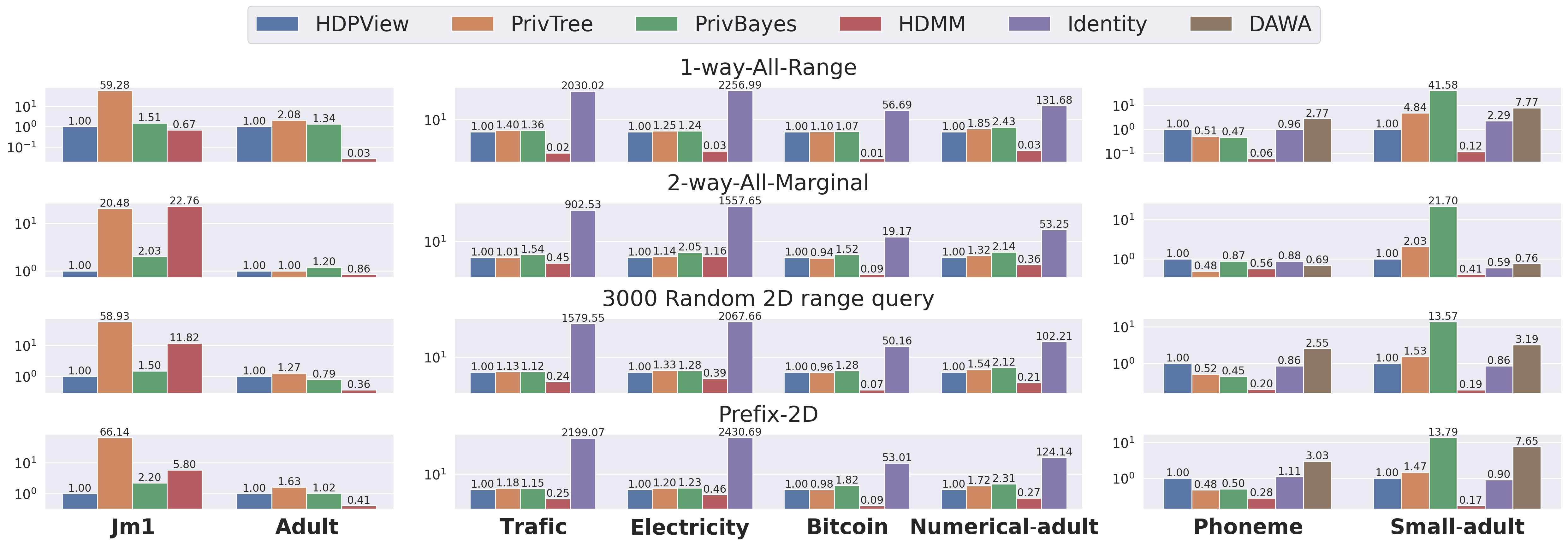
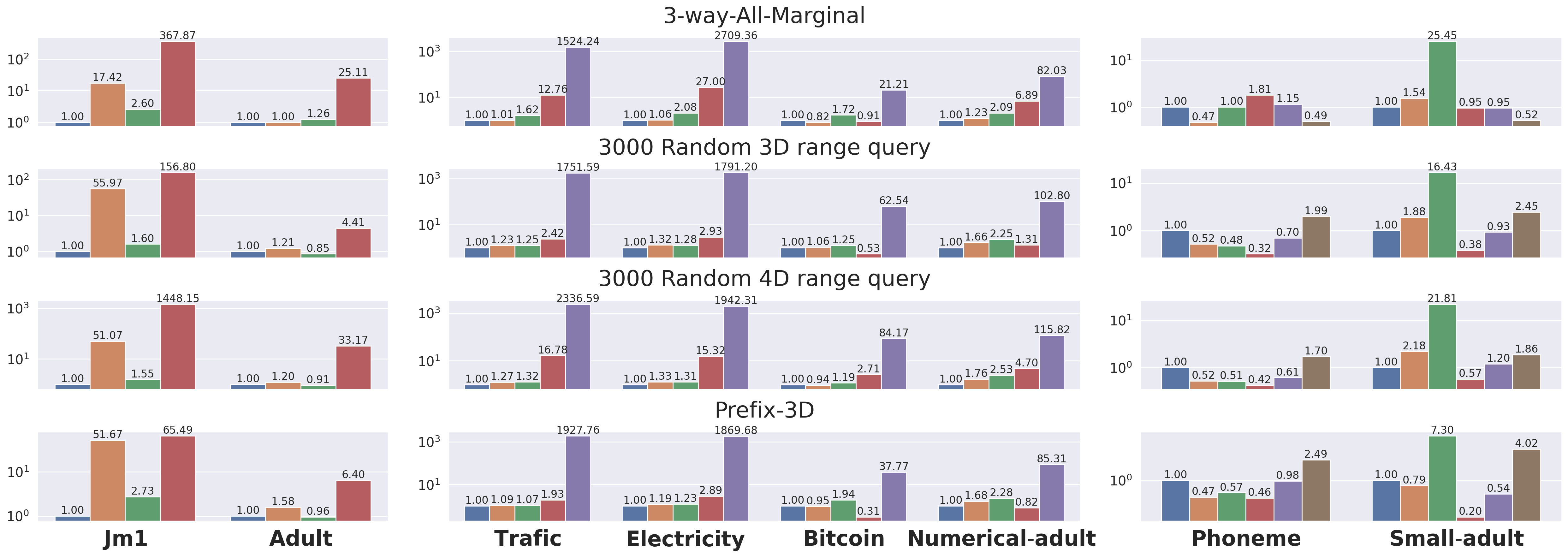
High quality on average. Figure 3 shows the relative RMSEs for all datasets and workloads and algorithms with privacy budget =1.0. The relative RMSE (log-scale) is plotted on the vertical axis and the dataset on the horizontal axis where high-dimensional datasets (Jm1 and Adult) are on the left, medium-dimensional datasets (Traffic, Electricity, Bitcoin and Numerical-adult) are in the middle, and low-dimensional datasets (Small-adult and Phoneme) are on the right. The errors with Identity for high-dimensional data are too large and are omitted for appearance. As a whole, HDPView works well. In Section 1, Table 2 shows the relative RMSE averaged over all workloads and all datasets in Figure 3, and HDPView achieves the lowest error on average. In data exploration, we want to run a variety of queries, so the average accuracy is important. We believe HDPView has such a desirable property. A detailed comparisons with the competitors are explained in the following paragraphs.
Comparison with Identity, HDMM and DAWA. Identity, which is the most basic Baseline, and HDMM, which performs workload optimization, cause more errors for high-dimensional datasets than HDPView. For Identity, the reason is that the accumulation of noise increases as the number of domains increases. HDPView avoids the noise accumulation by grouping domains into large blocks. The results of HDMM show that the increasing dimension of the dataset and the dimension of the query can increase the error. This is because the matrix representing the counting queries to which the matrix mechanism is applied becomes complicated, making it hard to find efficient budget allocations. This is why the accuracy of the 3- or 4-dimensional queries for Jm1 and Adult is poor with HDMM. In particular, the HDMM’s sensitivity to dimensionality increases can also be seen in Figure 7. DAWA’s partitioning leads more errors than the HDPView and Privtree. When applied to multi-dimensional data, DAWA finds the optimal partitioning on a domain mapped in one-dimension, while HDPView and Privtree finds more effective multi-dimensional data partitioning.
| #Blocks | 15669 |
| RMSE | 657.37 |
| #Blocks | 19475 |
| RMSE | 315.79 |
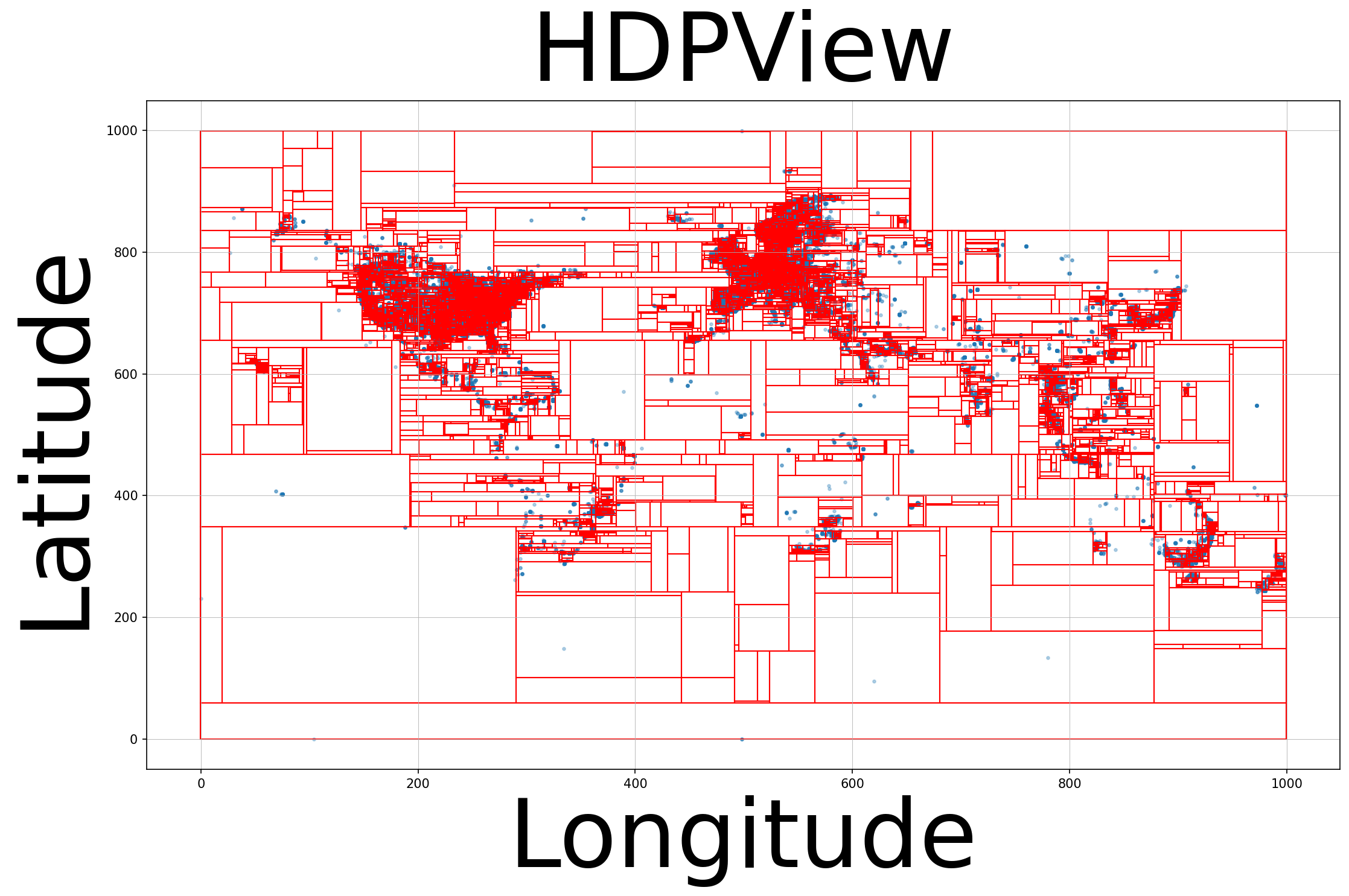
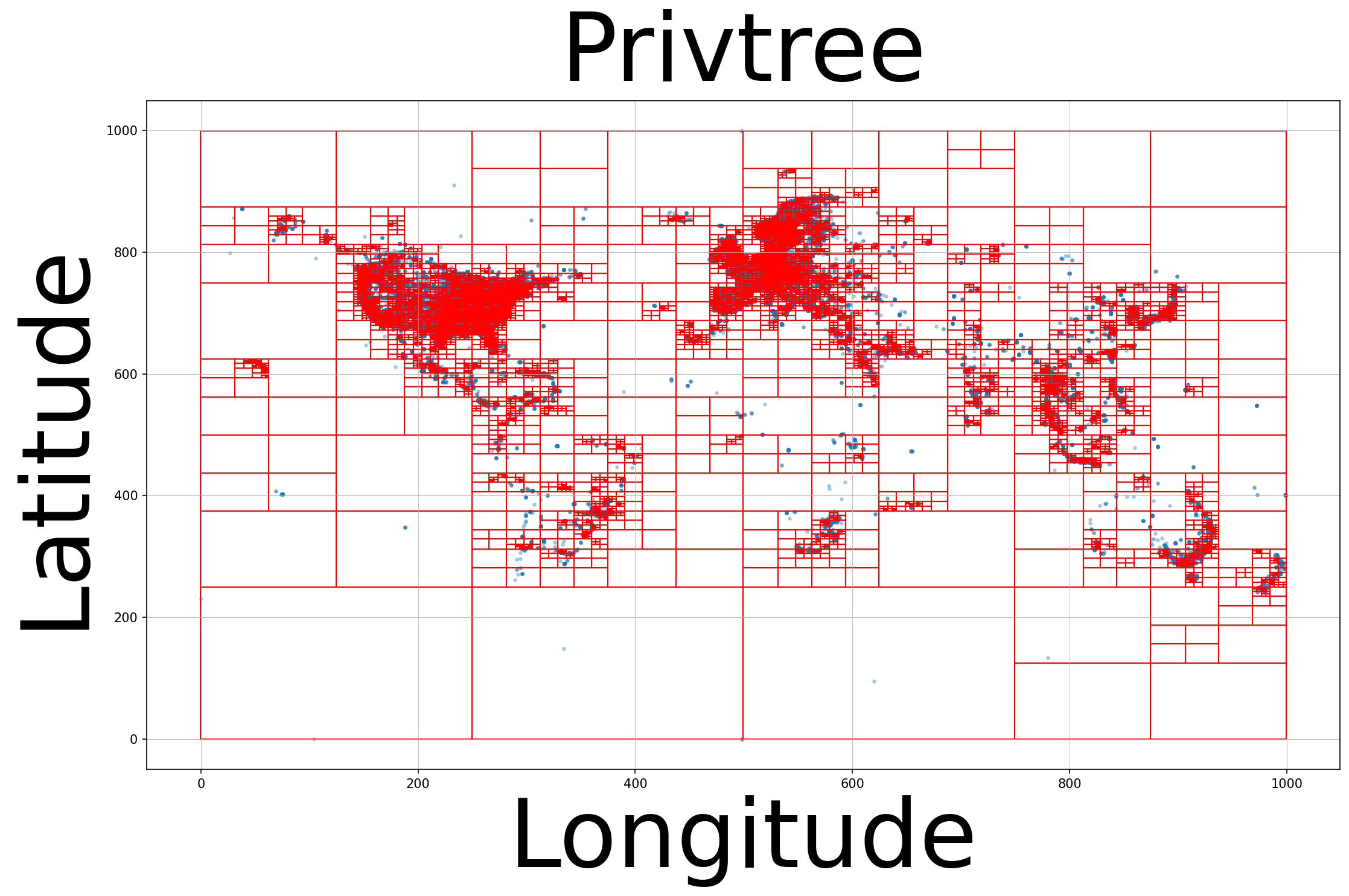
Comparison with Privtree. Overall, HDPView outperforms Privtree’s accuracy mainly for mid- to high-dimensional datasets. In particular, we can see Privtree’s performance drops drastically in high-dimensionality (i.e., Jm1). Privtree achieves higher accuracy than HDPView for Phoneme. This is likely because Privtree’s strategy, which prioritize finer splitting, are sufficient for the small domain size rather than HDPView’s heuristic algorithm. Even if the blocks is too fine, the accumulation of PEs is not so large in low-dimensionality, and AEs become smaller, which results in an accurate p-view. The reason why HDPView is better for Small-adult despite the low-dimensionality may be that the sizes of the cardinality of attributes are uneven (Small-adult: {74, 9, 5, 100}, Phoneme: {10, 10, 10, 10, 10, 10, 2}), which may make Privtree’s fixed cutting strategy ineffective. To see the very low-dimensional case, Figure 4 shows the block partitioning for the 2D data with a popular Gowalla (Leskovec, 2011) check-in dataset. The table below shows the number of blocks and the RMSE for the 3000 Random 2D range query. HDPView yields fewer blocks and Privtree generates a less noisy p-view for the abovementioned reason. The figure also confirms that HDPView performs a flexible shape of block partitioning.
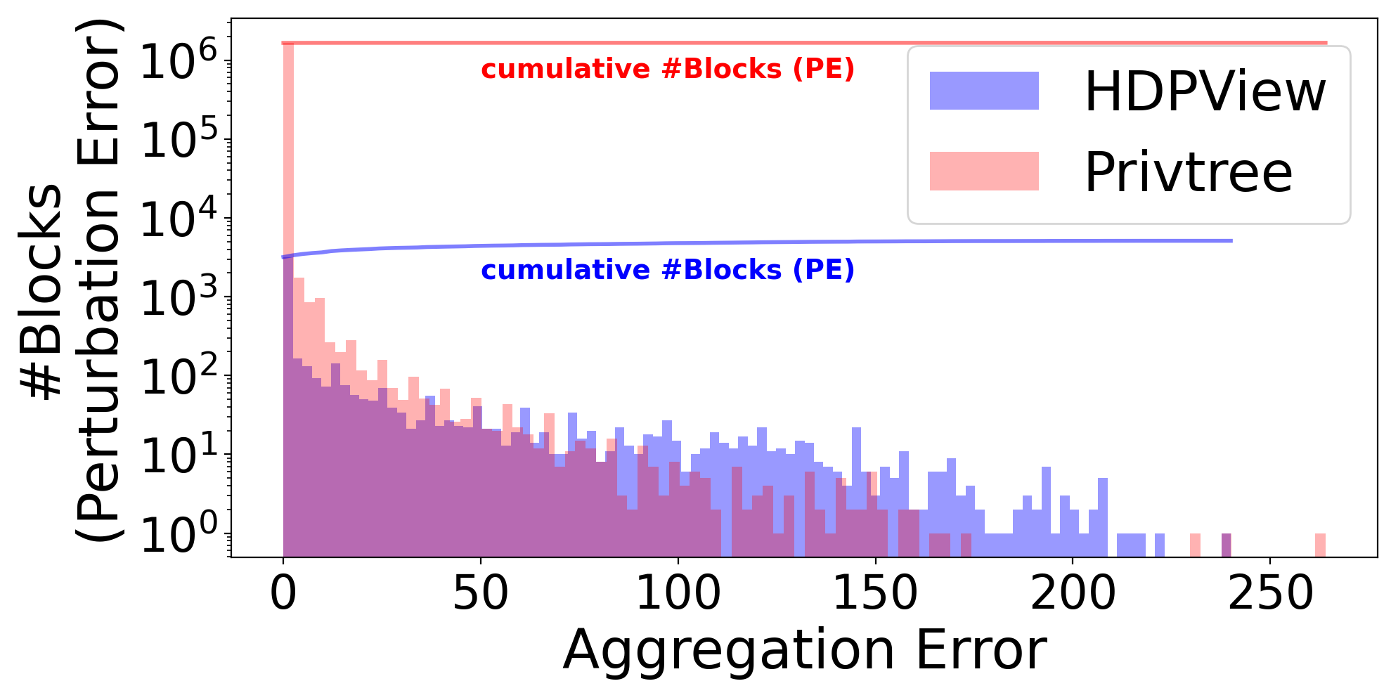
On the other hand, for high-dimensional dataset, this property can be avenged. In Privtree, a single cutting always generates new blocks, which are too fine, resulting in very large PEs even though the AEs are smaller. Figure 5 shows the distribution of AEs for blocks on Adult for HDPView and Privtree. HDPView has slightly larger AE blocks, but Privtree has a large number of blocks and cause larger PEs. An extreme case is Jm1 in which Privtree causes large errors. This is probably because Jm1 actually requires fewer blocks since the distribution is highly concentrated (c.f., Table 3). Figure 8 shows that the number of blocks of generated p-view by HDPView and Privtree. For Jm1, HDPView generates very small number of blocks while Privtree does not. We can confirm that HDPView avoids unnecessary splitting via random cut and suppresses the increase in PEs which causes in Privtree. This would be noticeable for datasets with concentrated distributions, where the required number of blocks is essentially small.
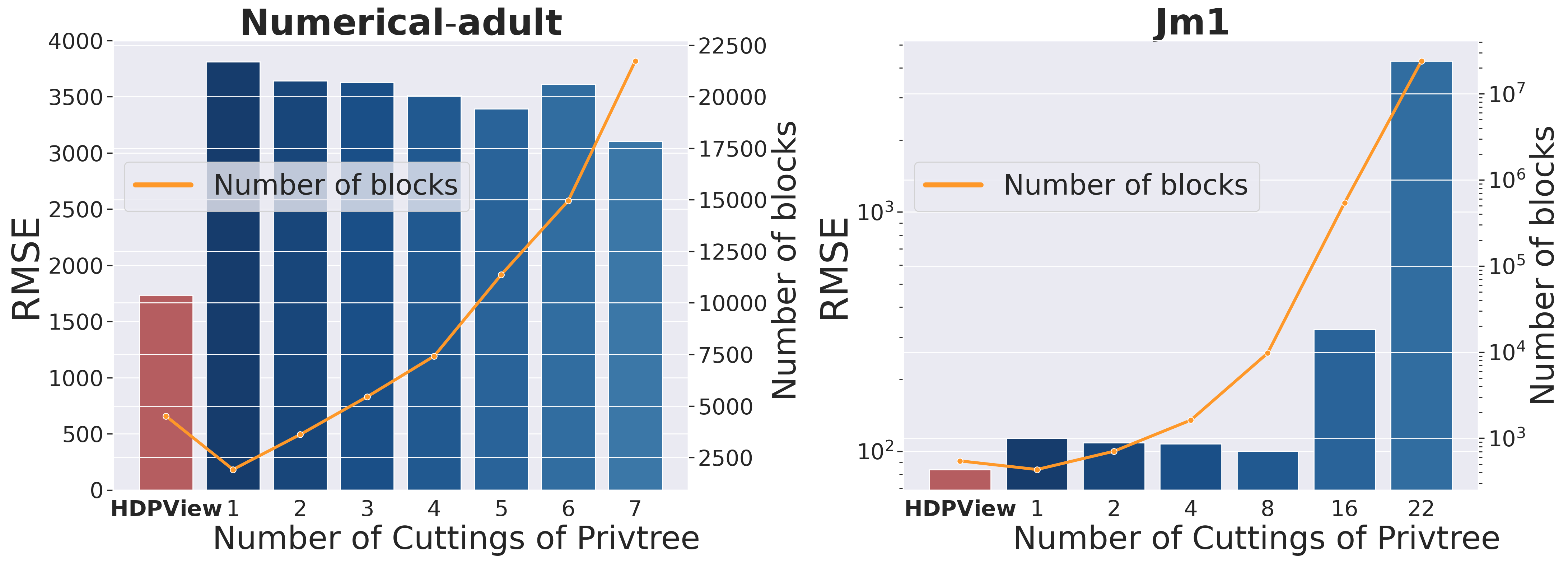
Figure 6 shows the results of reducing the number of cut attributes in Privtree and adjusting the number of blocks in p-view on Numerical-adult and Jm1. If the number of cut attributes is smaller than the dimension , we choose target attributes in a round-robin way (Appendix of (Zhang et al., 2016)). In the case of Numerical-adult, the error basically decreases as the number of cut attributes is increased, similar to the observation in Appendix of (Zhang et al., 2016). However, for high-dimensional data such as Jm1, the error increases rapidly as the number of cut attributes increases to some extent. This is consistent with the earlier observation that influence of PEs increases. Also, in any cases, the error of HDPView is smaller, indicating that HDPView not only has a smaller number of blocks, but also performs effective block partitioning compared to Privtree on these datasets.
Comparison with PrivBayes. We do not consider PrivBayes a direct competitor because it is a generative model approach that does not provide any analytical reliability as described in Section 2. However, PrivBayes is a state-of-the-art specialized for publishing differentially private marginal queries; therefore, we compared the accuracy to demonstrate the performance of HDPView. As shown in Figure 3, HDPView is a little more accurate than PrivBayes in many cases. However, in Adult, PrivBayes slightly outperforms HDPView. Because PrivBayes uses Bayesian network to learn the data distribution, it can fit well even to high-dimensional data as long as the distribution of the data is easily modelable. In HDPView, with larger dimensionality, the PEs grow slightly because the total number of blocks increases. The AEs also grow since more times of random converge result in larger errors. Thus, the total error is at least expected to increase, and the larger dimensionality may work to the advantage of PrivBayes. Still, HDPView is advantageous, especially for concentrated data such as Jm1.
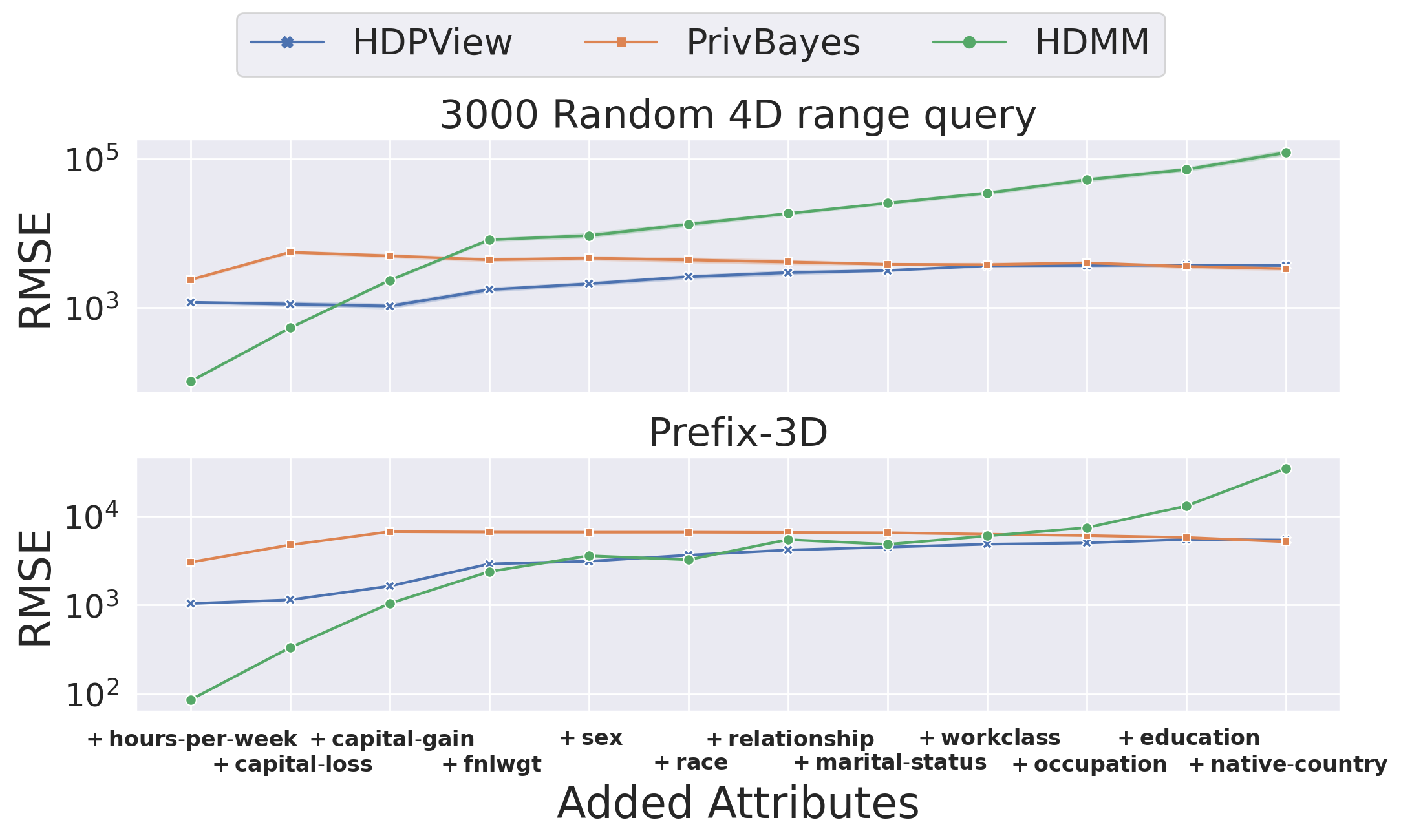
We consider the reason why on Numerical-adult, which has a smaller dimensionality than Adult, PrivBayes is less accurate than HDPView is because the effective attributes for capturing the accurate marginal distributions with Bayesian network are removed. We can see the same behavior for Small-adult. The following experimental results can support this. Figure 7 describes the changes in the RMSE with attributes added to Adult one by one in two workloads, where the added attributes are shown on the horizontal axis. Initially, HDPView is more accurate than PrivBayes. As attributes are added, HDPView is basically robust with increasing dimensionality, but the error increases slightly. On the other hand, interestingly, the error in PrivBayes becomes slightly smaller.
Lastly, considering HDPView is better in Numerical-adult and worse in Adult, one of the advantages of PrivBayes may be due to the increase in categorical attributes. Because HDPView bisects the ordered domain space, it may be hard to effectively divide categorical attributes, which possibly worsens the accuracy in HDPView.
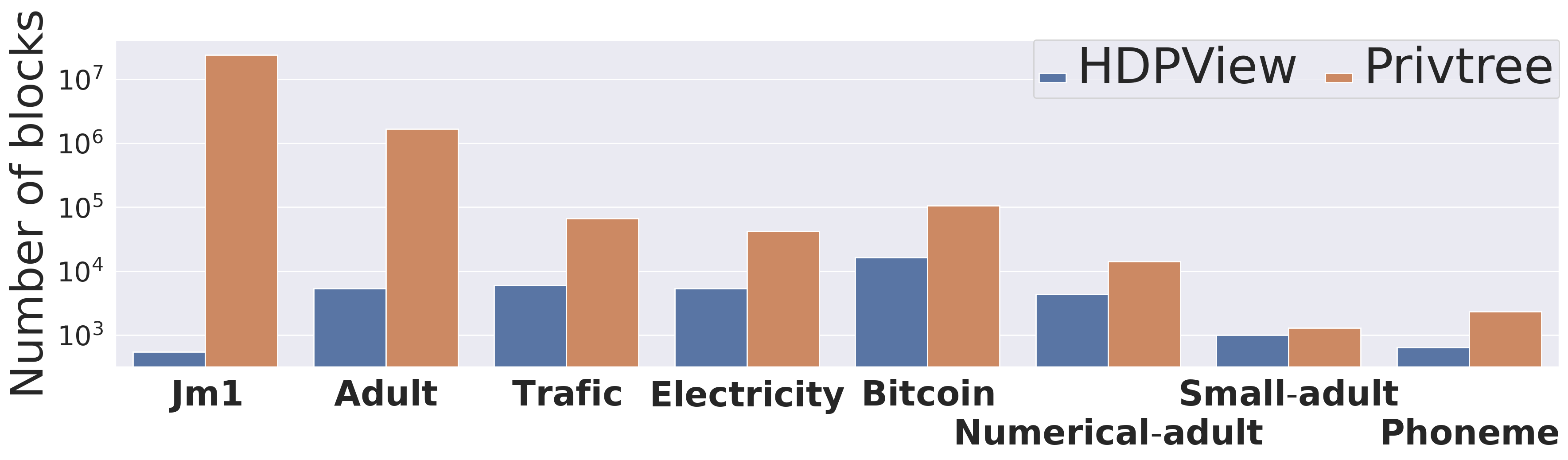
6.3. Space Efficiency
Our proposed p-view stores each block in a single record. This method avoids redundancy in recording all cells that belong to the same block. The p-view consists of blocks and values, and basically, the space complexity follows the number of blocks. Figure 8 shows a comparison between the numbers of blocks of HDPView and Privtree. While the accuracy of the counting queries of HDPView is higher than that of Privtree, the number of blocks generated by HDPView is much lower than that of Privtree, indicating that the strategy of HDPView avoids unnecessary splitting. In particular, on Jm1, HDPView is more efficient than Privtree. Table 4 shows the size of the randomized views, Identity-based noisy count vector (not p-view) and p-view generated by HDPView at =1.0. Since HDPView constructs the p-view by a compact representation, it results in up to times smaller space on Adult.
| Dataset | Identity-based | HDPView |
|---|---|---|
| Adult | 30.99 EB | 3.61 MB |
| Bitcoin | 1.27 TB | 6.77 MB |
| Electricity | 1.11 TB | 2.19 MB |
| Phoneme | 781.34 KB | 273.59 KB |
7. Conclusion
We addressed the following research question: How can we construct a privacy-preserving materialized view to explore the unknown properties of the high-dimensional sensitive data? To practically construct the p-view, we proposed a data-aware segmentation method, HDPView. In our experiments, we confirmed the following desirable properties, (1) Effectiveness: HDPView demonstrated smaller errors for various range counting queries in multidimensional queries. (2) Space efficiency: HDPView generates a compact representation of the p-view. We believe that our method helps us explore sensitive data in the early stages of data mining while preserving data utility and privacy.
References
- (1)
- dat (1996) 1996. Adult Data Set - UCI Machine Learning Repository. http://archive.ics.uci.edu/ml/datasets/Adult.
- dat (2014a) 2014a. electricity - OpenML. https://www.openml.org/d/151.
- dat (2014b) 2014b. jm1 - OpenML. https://www.openml.org/d/1053.
- dat (2015) 2015. phoneme - OpenML. https://www.openml.org/d/1489.
- dat (2019) 2019. Metro Interstate Traffic Volume Data Set - UCI Machine Learning Repository. http://archive.ics.uci.edu/ml/datasets/Metro+Interstate+Traffic+Volume.
- dat (2020) 2020. BitcoinHeistRansomwareAddressDataset Data Set - UCI Machine Learning Repository. https://archive.ics.uci.edu/ml/datasets/BitcoinHeistRansomwareAddressDataset.
- Abadi et al. (2016) Martin Abadi, Andy Chu, Ian Goodfellow, H Brendan McMahan, Ilya Mironov, Kunal Talwar, and Li Zhang. 2016. Deep learning with differential privacy. In Proceedings of the 2016 ACM SIGSAC Conference on Computer and Communications Security. ACM, 308–318.
- Abowd (2018) John M Abowd. 2018. The us census bureau adopts differential privacy. In Proceedings of the 24th ACM SIGKDD International Conference on Knowledge Discovery & Data Mining. 2867–2867.
- Acs et al. (2018) Gergely Acs, Luca Melis, Claude Castelluccia, and Emiliano De Cristofaro. 2018. Differentially private mixture of generative neural networks. IEEE Transactions on Knowledge and Data Engineering 31, 6 (2018), 1109–1121.
- Balas and Padberg (1976) Egon Balas and Manfred W Padberg. 1976. Set partitioning: A survey. SIAM review 18, 4 (1976), 710–760.
- Bindschaedler et al. (2017) Vincent Bindschaedler, Reza Shokri, and Carl A Gunter. 2017. Plausible deniability for privacy-preserving data synthesis. Proceedings of the VLDB Endowment 10, 5 (2017), 481–492.
- Chaudhuri et al. (2019) Kamalika Chaudhuri, Jacob Imola, and Ashwin Machanavajjhala. 2019. Capacity bounded differential privacy. In Advances in Neural Information Processing Systems. 3469–3478.
- Chen et al. (2015) Rui Chen, Qian Xiao, Yu Zhang, and Jianliang Xu. 2015. Differentially private high-dimensional data publication via sampling-based inference. In Proceedings of the 21th ACM SIGKDD International Conference on Knowledge Discovery and Data Mining. ACM, 129–138.
- Cormode et al. (2012) Graham Cormode, Cecilia Procopiuc, Divesh Srivastava, Entong Shen, and Ting Yu. 2012. Differentially private spatial decompositions. In 2012 IEEE 28th International Conference on Data Engineering. IEEE, 20–31.
- Dwork (2006) Cynthia Dwork. 2006. Differential privacy. In Proceedings of the 33rd international conference on Automata, Languages and Programming-Volume Part II. Springer-Verlag, 1–12.
- Dwork et al. (2014) Cynthia Dwork, Aaron Roth, et al. 2014. The algorithmic foundations of differential privacy. Found. Trends Theor. Comput. Sci. 9, 3-4 (2014), 211–407.
- Fan et al. (2020) Ju Fan, Junyou Chen, Tongyu Liu, Yuwei Shen, Guoliang Li, and Xiaoyong Du. 2020. Relational Data Synthesis Using Generative Adversarial Networks: A Design Space Exploration. Proc. VLDB Endow. 13, 12 (July 2020), 1962–1975. https://doi.org/10.14778/3407790.3407802
- Ge et al. (2019) Chang Ge, Xi He, Ihab F Ilyas, and Ashwin Machanavajjhala. 2019. Apex: Accuracy-aware differentially private data exploration. In Proceedings of the 2019 International Conference on Management of Data. 177–194.
- Ge et al. (2020) Chang Ge, Shubhankar Mohapatra, Xi He, and Ihab F Ilyas. 2020. Kamino: Constraint-Aware Differentially Private Data Synthesis. arXiv preprint arXiv:2012.15713 (2020).
- Harder et al. (2021) Frederik Harder, Kamil Adamczewski, and Mijung Park. 2021. DP-MERF: Differentially Private Mean Embeddings with RandomFeatures for Practical Privacy-preserving Data Generation. In International Conference on Artificial Intelligence and Statistics. PMLR, 1819–1827.
- Hay et al. (2009) Michael Hay, Vibhor Rastogi, Gerome Miklau, and Dan Suciu. 2009. Boosting the accuracy of differentially-private histograms through consistency. arXiv preprint arXiv:0904.0942 (2009).
- Johnson et al. (2018b) Noah Johnson, Joseph P Near, Joseph M Hellerstein, and Dawn Song. 2018b. Chorus: Differential privacy via query rewriting. arXiv preprint arXiv:1809.07750 (2018).
- Johnson et al. (2018a) Noah Johnson, Joseph P Near, and Dawn Song. 2018a. Towards practical differential privacy for SQL queries. Proceedings of the VLDB Endowment 11, 5 (2018), 526–539.
- Johnson and Lindenstrauss (1984) William B Johnson and Joram Lindenstrauss. 1984. Extensions of Lipschitz mappings into a Hilbert space 26. Contemporary mathematics 26 (1984).
- Jordon et al. (2018) James Jordon, Jinsung Yoon, and Mihaela van der Schaar. 2018. PATE-GAN: generating synthetic data with differential privacy guarantees. In International Conference on Learning Representations.
- Kotsogiannis et al. (2019) Ios Kotsogiannis, Yuchao Tao, Xi He, Maryam Fanaeepour, Ashwin Machanavajjhala, Michael Hay, and Gerome Miklau. 2019. PrivateSQL: a differentially private SQL query engine. Proceedings of the VLDB Endowment 12, 11 (2019), 1371–1384.
- Leskovec (2011) Jure Leskovec. 2011. Gowalla Dataset. http://snap.stanford.edu/data/loc-Gowalla.html.
- Li et al. (2014) Chao Li, Michael Hay, Gerome Miklau, and Yue Wang. 2014. A Data- and Workload-Aware Algorithm for Range Queries under Differential Privacy. Proc. VLDB Endow. 7, 5 (Jan. 2014), 341–352. https://doi.org/10.14778/2732269.2732271
- Li et al. (2015) Chao Li, Gerome Miklau, Michael Hay, Andrew McGregor, and Vibhor Rastogi. 2015. The matrix mechanism: optimizing linear counting queries under differential privacy. The VLDB journal 24, 6 (2015), 757–781.
- McKenna et al. (2018) Ryan McKenna, Gerome Miklau, Michael Hay, and Ashwin Machanavajjhala. 2018. Optimizing Error of High-Dimensional Statistical Queries under Differential Privacy. Proc. VLDB Endow. 11, 10 (June 2018), 1206–1219. https://doi.org/10.14778/3231751.3231769
- McSherry (2009) Frank D McSherry. 2009. Privacy integrated queries: an extensible platform for privacy-preserving data analysis. In Proceedings of the 2009 ACM SIGMOD International Conference on Management of data. 19–30.
- Papernot et al. (2016) Nicolas Papernot, Martín Abadi, Ulfar Erlingsson, Ian Goodfellow, and Kunal Talwar. 2016. Semi-supervised knowledge transfer for deep learning from private training data. arXiv preprint arXiv:1610.05755 (2016).
- Qardaji et al. (2013) Wahbeh Qardaji, Weining Yang, and Ninghui Li. 2013. Differentially private grids for geospatial data. In 2013 IEEE 29th international conference on data engineering (ICDE). IEEE, 757–768.
- Qardaji et al. (2014) Wahbeh Qardaji, Weining Yang, and Ninghui Li. 2014. Priview: practical differentially private release of marginal contingency tables. In Proceedings of the 2014 ACM SIGMOD international conference on Management of data. 1435–1446.
- Ren et al. (2018) Xuebin Ren, Chia-Mu Yu, Weiren Yu, Shusen Yang, Xinyu Yang, Julie A McCann, and S Yu Philip. 2018. LoPub: High-Dimensional Crowdsourced Data Publication with Local Differential Privacy. IEEE Transactions on Information Forensics and Security 13, 9 (2018), 2151–2166.
- Rogers et al. (2020) Ryan Rogers, Subbu Subramaniam, Sean Peng, David Durfee, Seunghyun Lee, Santosh Kumar Kancha, Shraddha Sahay, and Parvez Ahammad. 2020. LinkedIn’s Audience Engagements API: A privacy preserving data analytics system at scale. arXiv preprint arXiv:2002.05839 (2020).
- Su et al. (2020) Du Su, Hieu Tri Huynh, Ziao Chen, Yi Lu, and Wenmiao Lu. 2020. Re-identification Attack to Privacy-Preserving Data Analysis with Noisy Sample-Mean. In Proceedings of the 26th ACM SIGKDD International Conference on Knowledge Discovery & Data Mining. 1045–1053.
- Takagi et al. (2021) Shun Takagi, Tsubasa Takahashi, Yang Cao, and Masatoshi Yoshikawa. 2021. P3GM: Private high-dimensional data release via privacy preserving phased generative model. In 2021 IEEE 37th International Conference on Data Engineering (ICDE). IEEE, 169–180.
- Wang et al. (2019) Zhen Wang, Xiang Yue, Soheil Moosavinasab, Yungui Huang, Simon Lin, and Huan Sun. 2019. Surfcon: Synonym discovery on privacy-aware clinical data. In Proceedings of the 25th ACM SIGKDD International Conference on Knowledge Discovery & Data Mining. 1578–1586.
- Wilson et al. (2019) Royce J Wilson, Celia Yuxin Zhang, William Lam, Damien Desfontaines, Daniel Simmons-Marengo, and Bryant Gipson. 2019. Differentially private sql with bounded user contribution. arXiv preprint arXiv:1909.01917 (2019).
- Xiao et al. (2012) Yonghui Xiao, Li Xiong, Liyue Fan, and Slawomir Goryczka. 2012. DPCube: Differentially private histogram release through multidimensional partitioning. arXiv preprint arXiv:1202.5358 (2012).
- Xu et al. (2017) Chugui Xu, Ju Ren, Yaoxue Zhang, Zhan Qin, and Kui Ren. 2017. DPPro: Differentially Private High-Dimensional Data Release via Random Projection. IEEE Transactions on Information Forensics and Security 12, 12 (2017), 3081–3093. https://doi.org/10.1109/TIFS.2017.2737966
- Yaroslavtsev et al. (2013) Grigory Yaroslavtsev, Graham Cormode, Cecilia M Procopiuc, and Divesh Srivastava. 2013. Accurate and efficient private release of datacubes and contingency tables. In 2013 IEEE 29th International Conference on Data Engineering (ICDE). IEEE, 745–756.
- Zhang et al. (2017) Jun Zhang, Graham Cormode, Cecilia M Procopiuc, Divesh Srivastava, and Xiaokui Xiao. 2017. Privbayes: Private data release via bayesian networks. ACM Transactions on Database Systems (TODS) 42, 4 (2017), 25.
- Zhang et al. (2016) Jun Zhang, Xiaokui Xiao, and Xing Xie. 2016. Privtree: A differentially private algorithm for hierarchical decompositions. In Proceedings of the 2016 International Conference on Management of Data. ACM, 155–170.
- Zhang et al. (2014) Xiaojian Zhang, Rui Chen, Jianliang Xu, Xiaofeng Meng, and Yingtao Xie. 2014. Towards Accurate Histogram Publication under Differential Privacy. In Proceedings of the 2014 SIAM International Conference on Data Mining, Philadelphia, Pennsylvania, USA, April 24-26, 2014, Mohammed Javeed Zaki, Zoran Obradovic, Pang-Ning Tan, Arindam Banerjee, Chandrika Kamath, and Srinivasan Parthasarathy (Eds.). SIAM, 587–595. https://doi.org/10.1137/1.9781611973440.68
- Zhang et al. (2021) Zhikun Zhang, Tianhao Wang, Ninghui Li, Jean Honorio, Michael Backes, Shibo He, Jiming Chen, and Yang Zhang. 2021. PrivSyn: Differentially Private Data Synthesis. In USENIX Security Symposium.
- Zheng et al. (2019) Zhigao Zheng, Tao Wang, Jinming Wen, Shahid Mumtaz, Ali Kashif Bashir, and Sajjad Hussain Chauhdary. 2019. Differentially private high-dimensional data publication in internet of things. IEEE Internet of Things Journal 7, 4 (2019), 2640–2650.
Appendix A Analysis for Hyperparameters
We provide an explanation of the hyperparameters of HDPView. As shown in Algorithm 1, HDPView requires four main hyperparameters, , , and . We mentioned in Section 6.1 that we fix the hyperparameters as in our experiments. Here, we provide some insights into each hyperparameter from observations of experimental results on a real-world dataset Small-adult varying each hyperparameter.
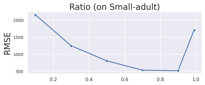
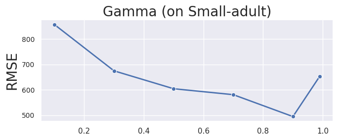
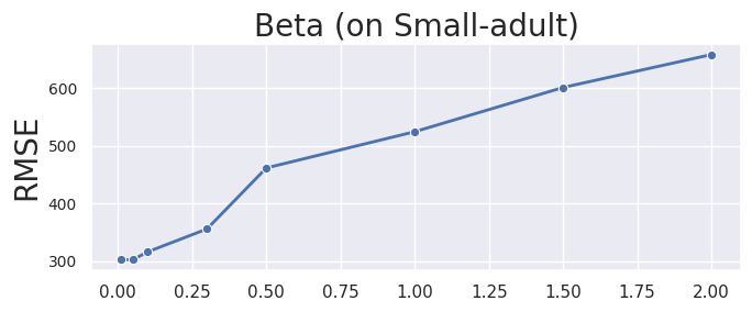
Figures 9 10 11 13 show the RMSEs for 3000 random 2D range query on Small-adult dataset when only one of the hyperparameters varies and others are fixed as the abovementioned default. From this result, we obtain the following insights:
Ratio, . The best accuracy is achieved when the Ratio is approximately 0.7~0.9 as shown in Figure 9. In HDPView, seemingly, the effect of aggregation error is larger than perturbation error, therefore we try to allocate a budget to the cutting side so that the aggregation error is smaller.
Gamma, . As shown in Figure 10, it was confirmed that prioritizing therandom converge to accurately determine AEs improves accuracy rather than random cut. However, if no budget is allocated for random cut, the error increases, i.e., a completely random cutting strategy lose accuracy compared to appropriate our proposed random cut. Therefore, 0.9 is reasonable. However, the random cut may be less less significant due to the conservative setting of the shown below.
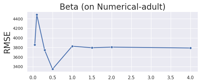
Beta, . The is somewhat conservatively determined. We choose because, when , the maximum depth of HDPView ’s bisection rarely reaches on various datasets. As a rough guideline, if the total number of domains in a given dataset is , all blocks can be split at times depth, assuming the domains are bisected exactly in the all cutting. Thus is deep enough to split all the blocks, allowing for some skewness, and all the cutting point is likely to be selected by an Exponential Mechanism rather than by random one. However, remember the budget for each EM is inversely proportional to , depending on the data set, the budget available for EM may be unnecessarily small due to the unnecessarily large setting of as is the case with Small-adult (Figure 11). We also show the Numerical-adult result as another example (Figure 12). The small do not take full advantage of the random cut. Since determining the optimal for any dataset is impossible without additional privacy consumption, we conservatively set for all dataset in the experiment.
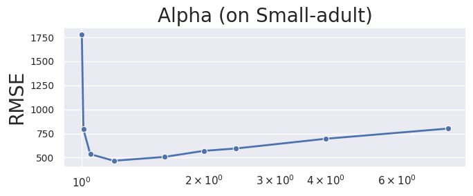
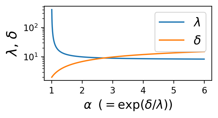
Alpha, . , i.e., , is valid for . If is extremely close to 1, diverges and HDPView does not work well because random converge causes large errors. Because and , as increases, decreases and converges to 3, but increases. Thus and are trade-offs. When increases, the bias of BAE increases, which also leads to a worse convergence decision. Figure 14 plots the size of and for various when . As increases, the increases, but the decrease in is small, starting from approximately 1.4. Therefore, around works well empirically and we use as default value.