HEAL: Brain-inspired Hyperdimensional Efficient Active Learning
Abstract
Drawing inspiration from the outstanding learning capability of our human brains, Hyperdimensional Computing (HDC) emerges as a novel computing paradigm, and it leverages high-dimensional vector presentation and operations for brain-like lightweight Machine Learning (ML). Practical deployments of HDC have significantly enhanced the learning efficiency compared to current deep ML methods on a broad spectrum of applications. However, boosting the data efficiency of HDC classifiers in supervised learning remains an open question.
In this paper, we introduce Hyperdimensional Efficient Active Learning (), a novel Active Learning (AL) framework tailored for HDC classification. proactively annotates unlabeled data points via uncertainty and diversity-guided acquisition, leading to a more efficient dataset annotation and lowering labor costs. Unlike conventional AL methods that only support classifiers built upon deep neural networks (DNN), operates without the need for gradient or probabilistic computations. This allows it to be effortlessly integrated with any existing HDC classifier architecture. The key design of is a novel approach for uncertainty estimation in HDC classifiers through a lightweight HDC ensemble with prior hypervectors. Additionally, by exploiting hypervectors as prototypes (i.e., compact representations), we develop an extra metric for to select diverse samples within each batch for annotation. Our evaluation shows that surpasses a diverse set of baselines in AL quality and achieves notably faster acquisition than many BNN-powered or diversity-guided AL methods, recording 11 to 40,000 speedup in acquisition runtime per batch.
Brain-inspired Computing, Active Learning, Hyperdimensional Computing
1 Introduction
The unparalleled performance of modern Machine Learning (ML) techniques such as Deep Neural Networks (DNN) is underpinned by the availability of vast and diverse data sources, facilitating ML applications in myriad real-world scenarios. Although beneficial for complex tasks, DNNs suffer from computational inefficiencies primarily due to their large model sizes and resource-demanding learning process [1, 2]. Consequently, DNNs are less suitable for edge and real-time applications. Conversely, an emerging and brain-inspired computing paradigm named HyperDimensional Computing (HDC) has shed light on a more lightweight path toward learning and reasoning [3, 4, 5, 6].
The human brain can process and retrieve information with remarkable robustness and efficiency based on neural signals with high dimensions [7]. In HDC, this motivates researchers to encode inputs to high-dimensional vector representations, i.e., hypervectors [8]. Building upon this hypervector encoding, previous works provide a well-defined set of hypervector operations for symbol representation, concept manipulation, and crucially, model learning [9, 3]. These operations are also designed to closely mimic human brain functionalities [10], fostering efficient learning, memorization, and information retrieval. In real-world implementations, HDC distinguishes itself from DNN by leveraging its hardware-friendly and straightforward mathematical operations to ensure lightweight and parallelizable processing [11, 12, 13], making it particularly suitable for swift online learning with limited computing resources [4, 14].
In the prevalent supervised learning scenario, a faster learner like HDC is undoubtedly important for lowering the learning cost. Nonetheless, the cost of acquiring labeled data cannot be ignored given the high costs and labor intensity of annotation. This poses a major challenge nowadays since the success of current ML algorithms is coupled with the cost of obtaining sufficient high-quality labeled data beforehand. Especially, with the model complexity growing, learning supervised DNN becomes significantly more data-demanding. While HDC surpasses DNN in learning efficiency, especially regarding model training iterations and runtime, it still significantly benefits from larger labeled datasets to achieve superior learning quality [13, 4]. Therefore, it is worthwhile investigating lightweight HDC learning with improved data efficiency.
We will focus on a specific strategy for improving data efficiency in this paper, namely Active Learning (AL). AL is a technique that reduces the annotation cost in data-centric and expert-driven supervised ML tasks. It proactively identifies unlabeled data that is deemed beneficial for subsequent training [15]. This contrasts with conventional supervised ML where the model passively learns from existing labeled data; yet, not all data points are equally important and indiscriminately labeling data points could be a waste of precious annotation budget (both time and financial). Therefore, prior research has introduced various AL strategies for data-intensive DNNs to prioritize annotating data points that are more informative than others. Model uncertainty quantization [16, 17], representative data sampling [18], and information-theory-based AL [19] rank among the most widely applied methods.
Most AL methods are designed to work side by side with DNNs, utilizing the gradient information, embeddings, or output logits of neural networks to shape the AL acquisition strategy [16, 17, 20, 19]. However, having to rely on inefficient DNN backbones means that their overall efficiency is limited. Apart from this, existing AL methods also show significant overhead, in terms of how long it takes to acquire a batch of new data points. For example, representative sampling methods require pair-wise comparison throughout the dataset and sequential greedy acquisition [18]; both incur high computation overhead and poor scalability. Uncertainty-based and information-theoretical AL methods leverage Bayesian Neural Networks (BNN) to properly quantify model uncertainty and predictive probability. However, it is well known that BNNs have even worse learning and inference efficiency when compared to regular DNNs [21, 22, 23, 24]. Existing BNN methods mainly rely on variational inference to approximate the model posterior and the marginal predictive distribution [23, 21]. These methods vary in their implementation of variational inference and generate final predictive probability, and thus they also have different sources of inefficiency.
In this paper, we present , an AL methodology that leverages brain-inspired hypervector operations to further refine HDC-based ML, enhancing sample efficiency and addressing the limitations of existing AL methods. Our contributions are summarized as follows:
-
•
To the best of our knowledge, is the first AL algorithm specifically designed for HDC-based ML. Prior HDC algorithms require the training dataset to be as complete as possible to ensure the highest learning quality. However, proactively annotates unlabeled data points via uncertainty and diversity-guided acquisition, leading to a more efficient dataset annotation and lowering the labor cost.
-
•
Implementing AL within the HDC context presents significant challenges, as conventional approaches rely on BNNs and gradient-based learning for uncertainty estimation and diversity metrics. In contrast, is gradient-free and seamlessly integrates with any pre-existing HDC classifier architecture.
-
•
Within the framework of , we introduce a novel approach for uncertainty estimation in HDC classifiers through a lightweight HDC ensemble with prior hypervectors. The AL acquisition metric is based on average similarity margins across sub-models. Furthermore, leveraging hypervector memorization, we develop an extra metric for to acquire diverse samples in batch-mode AL.
-
•
Comprehensive comparison reveals that outperforms in terms of AL quality and data efficiency against a diverse set of baselines on four distinct datasets. Meanwhile, achieves notably faster acquisition than many BNN-powered or diversity-guided AL methods, recording 11 to 40,000 speedup in terms of acquisition runtime per batch.
As for the organization of this paper: In Section 2, we summarize the prior works, challenges, and necessary concepts regarding AL, Bayesian inference, and HDC. In Section 3, we discuss our design in to enable uncertainty estimation in HDC classification algorithms, compare several algorithm design choices, and introduce techniques to enhance the overall efficiency. We present the AL algorithm with the proposed diversity metric in Section 4 and evaluate its performance against several baselines in Section 5.
2 Background & Related Works
In this section, we formally define the problem setting for AL and cover the related AL notations that will be used in this paper (Section 2.1). Since a great many AL methods are powered by Bayesian inference, we introduce the necessary backgrounds for Bayesian inference methods in Section 2.2, especially ones that are related to BNNs. Apart from AL techniques using BNNs, we also consider general AL methods used in deep learning and analyze the challenges in existing algorithm designs (Section 2.3). Last but not least, for readers that are not familiar with HDC, we include a concise but comprehensive introduction as well as representative related works in Section 2.4.
2.1 Problem Settings for Active Learning
In this paper, we focus on a multi-class classification problem, with being the instance space and being the label space. Suppose that there are different classes in : . We are interested in a classifier that predicts the label of each instance, which can be regarded as a mapping function . stands for the classifier parameters. For the case of AL, we assume that the classifier is trained in a supervised way; however, instead of having a large labeled dataset in the beginning, the classifier starts training with a small labeled training set and the size of training set will gradually growing as the AL algorithm kicked in. This particular training procedure is known as pool-based AL since there is a relatively large pool of unlabeled data . As regular supervised learning, a testing or validation dataset is used for evaluation.
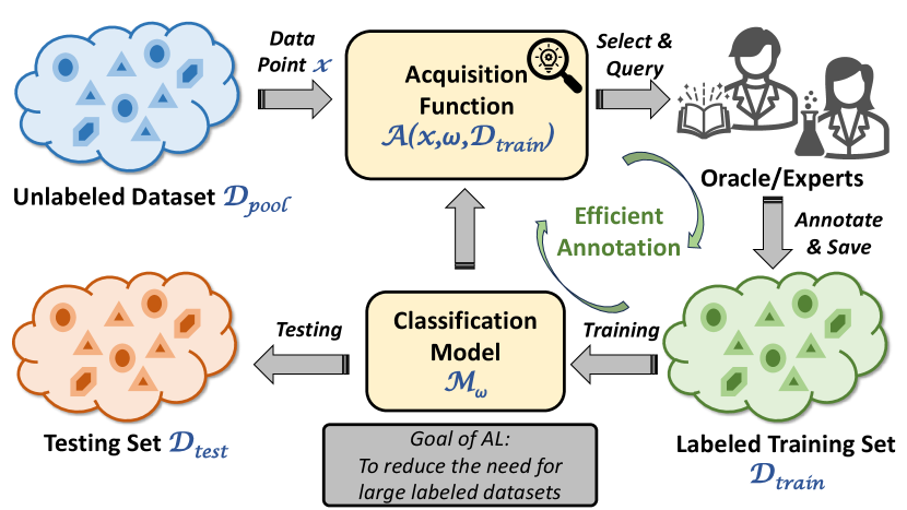
Fig. 1 presents the procedure of AL, which includes an oracle to provide extra labeled data points. The oracle can give the correct label for every data point in as long as the annotation request is made from AL. The labeled data points are then removed from and added to the training dataset . The goal of AL, in short, is to minimize the number of annotation requests (also the size of the labeled dataset) while ensuring satisfying prediction accuracy. Specifically, at each step, AL uses an acquisition function to rank samples in and select extra data that maximizes this function, given the current classifier trained using :
| (1) |
In practice, AL algorithms usually acquire a batch of new data points instead of only one at each step to reduce the frequency and cost of model retraining. This can be achieved by simply acquiring top data points according to the acquisition function . Sometimes, it is also required to slightly modify the acquisition function [19] or add extra metrics [16] to maintain the diversity in acquired batches. (more details in Section 4.2).
2.2 Bayesian Inference for DNNs
Bayesian inference plays a key role in uncertainty-based AL as it provides a principled way of understanding the uncertainty inherent in predictions [19, 15]. In Bayesian inference, the neural networks are no longer modeled in static weights but stochastically in a distribution [25]. It is known as the posterior distribution whose variance quantifies the belief in DNN weights given the seen data points in training. This also means a prior belief exists before training. Using the posterior, the predictive distribution is calculated as: . We can compute the posterior using the Bayes Theorem as follows:
| (2) |
with being the likelihood. From the equation above, it is clear that the exact posterior will be intractable in DNNs because the weight space is generally high-dimensional and takes exponential time to evaluate the integral in the denominator [23].
Therefore, approximating the posterior in a more tractable way is fundamental for achieving Bayesian inference in DNNs. Variational Inference (VI) has been a widely applied method that replaces the original with a simpler variational distribution with a tractable , e.g., a family of Gaussian distributions [22, 21]. This is usually achieved by minimizing the Kullback-Leibler (KL) divergence that measures the differences between two probability distributions. By rearranging the terms in the KL divergence, we get Evidence Lower Bound (ELBO).
Early works that tried to apply VI for DNNs built up the foundation for what we know today as Bayesian Neural Networks (BNN) [26, 27, 28]. However, they faced several challenges such as the lack of support for modern DNNs and scalability to larger datasets [29]. More recent BNN works [21, 22, 23] make it practical to apply Bayesian inference for deep learning tasks, thanks to their compatibility with most DNN structures and mini-batch gradient descent optimization.
Apart from VI-based BNNs, researchers also develop methods based on ensemble learning for uncertainty estimation in DNNs. For example, MC-Dropout [24] proposes to approximate Bayesian inference by adding dropout layers. In its design, dropout layers are enabled also in network inference instead of just during training. The predictive distribution and uncertainty are derived from these multiple forward passes, assuming that the predictions follow a Gaussian distribution. On the other hand, Deep Ensemble [30] more explicitly utilizes the ensemble of DNNs with bootstrapping and adversarial training. For classification problems, the predictive probabilities are computed as the average of ensemble softmax probabilities. Prior works [31, 32] also show that Deep Ensemble generally achieves the best performance on uncertainty estimation, compared to the implicit ensemble in MC-Dropout and VI-based BNN.
2.3 Existing DNN-AL Methods and Their Challenges
As is pointed out in the introduction, one motivation of this paper is that current AL methods face various kinds of inefficiencies; these challenges are the consequences of using acquisition functions with high overhead as well as relying on computation-heavy DNNs (or BNNs) for training and inference.
Uncertainty-based AL: Many existing AL methods are based on a certain uncertainty metric. For example, confidence sampling [33] will select samples with the smallest predictive probability while entropy sampling [34] selects points with the highest predictive entropy values . Both confidence and entropy provide direct estimations of model uncertainty [20]. Margin sampling [35, 36, 37] approaches this at a slightly different angle, where it sorts samples in the AL pool according to the probability margin . Here stands for the predicted label and is the class with the second largest predictive probability. The data point with the smallest margin indicates low confidence in prediction and will be annotated by experts.
However, the aforementioned methods generally have significant acquisition costs as they require BNN during uncertainty estimation. As for the BNNs mentioned above in 2.2, they all show overheads in different aspects. First, to obtain the predictive distribution, methods like MC-Dropout and Bayes-by-Backprop require more than 100 forward inferences on one single test sample. The inefficient BNN inference directly leads to a higher acquisition cost since every AL step requires scoring all data in . The same is true for Deep Ensemble where the inference is inefficiently carried out on multiple sub-models. Second, training BNNs is notably more costly than regular DNNs using similar architectures. For example, network parameters are doubled in BNNs that parameterize the variance of weights [23], and they can have poor scalability to dataset sizes [38].
In addition, AL methods with only the uncertainty metric are prone to sample duplicate data points in the batch acquisition, compromising the advantage in data efficiency. The next few categories of AL methods mitigate this problem by explicitly or implicitly considering the diversity in batch acquisition. However, they have also shown significantly higher overhead in acquisition.
Information Theory Based AL: AL methods [15, 19] also utilize information theory such as the mutual information (also known as the expected information gain) to guide the acquisition. Here we show the definition of mutual information in batch acquisition (i.e., BatchBALD [19]):
|
|
(3) |
Notice that we omit the conditioning on for each term in this equation. The first term on the right side of the equation represents the overall predictive uncertainty with the unconditioned entropy while the second term is the expected conditional entropy for each sampled model. In short, this acquisition function looks for data points on which sampled models (from the posterior ) disagree with each other.
As for the drawbacks, they still suffer from the overhead of Bayesian inference and posterior computation, since the information metric selected will only be helpful and properly calibrated with Bayesian inference. In addition, computing equation 3 in each step of batch acquisition is time-consuming and memory-heavy as the complexity grows exponentially with the batch sizes [19]. With a batch size larger than 10, the acquisition runtime can become inhabitable for deployment on CPUs or any resource-limited hardware.
Representative Sampling Based AL: Algorithms in this group aim to find a subset of data points that can behave as a surrogate for the complete training dataset, which is an intuitive method to reduce the annotation cost while ensuring learning quality. The core-set method [18, 39] achieves this goal by leveraging the geometry of the data points and minimizing the covering radius of the selected subset, where a smaller covering radius means a better surrogate. However, the computational cost remains high for this method because it requires computing pairwise distances for every point to be added in the representative subset; this limits the scalability and deployments of this method.
Hybrid AL Methods: Work in [17] applies meta-learning to help balance the part that follows the representative sampling and the part for uncertainty-based sampling. Work in [40] also aims to acquire data points that are diverse and informative. A more recent work [16] proposes BADGE, a diversity and uncertainty-guided AL framework for DNNs, that leverages the magnitude of gradient embedding as the sign for uncertainty. It then applies the k-MEANS++ algorithm [41] on these hallucinated gradients to ensure diversity. However, the cost of running k-MEANS++ adds significant overhead to the AL acquisition process.
2.4 Brain-inspired HDC
The human brain is a very efficient and robust learning machine and inspires many different machine learning algorithms. HDC, as our focus in this paper, utilizes high-dimensional representations to emulate brain functionalities for ML tasks. Representations in HDC are considered holographic since the information is evenly distributed among all dimensions of the hypervector [3]; therefore, corruption or noises on some dimensions will not lead to catastrophic information loss [42].
As the background, we start with how HDC represents symbols and memorizes concepts in a structured way. Suppose there are three different symbols , , and , we map them to three randomly-sampled hypervector representations , , and with dimensionality . More specifically, every element in those hypervectors is i.i.d. usually following a symmetric, zero-mean distribution [9]. For example, can be bipolar high-dimensional vectors, whose elements are either +1 or -1 with equal probability [3]. Hypervectors can represent not only individual symbols but also a combination or association of multiple symbols, which is enabled by the following three fundamental hypervector operations.
-
•
Hypervector Similarity () represents how close two hypervectors are in the hyperspace, defined based on the normalized dot product: . When is in the range of several hundred to around ten thousand, the similarity between any two random hypervectors is nearly zero (also known as near-orthogonal) because of the property of high-dimensional space.
-
•
Bundling () in HDC means the element-wise addition of two or more hypervectors. This creates a new hypervector that represents the set of hypervectors and thus remains similar to all its constituents. Suppose we have , and then we check the similarity between the bundled hypervector and each symbol hypervector: while .
-
•
Binding () stands for the element-wise multiplication of two hypervectors. It generates a dissimilar vector representing their association. To associate with , we bind their corresponding hypervectors: . Unlike bundling, is dissimilar to both constituents, e.g., .
The bundling operation is usually used when creating HDC-based ML models such as the classifier hypervectors and regression model hypervectors. The binding operation is used when associating features and values. We will cover more details regarding the usage of hypervector operations in Section 3.1.
In the past few years, HDC has gained significant traction as an emerging computing paradigm, especially for its deployments in machine learning and reasoning tasks. Prior works have proposed HDC-based algorithms and learning frameworks for classification [43, 4, 44], clustering [45, 46], regression [47, 9], and reinforcement learning [14, 48, 49] problems, showing the benefit of fast convergence in learning, high power/energy efficiency, natural data reuse and acceleration on customized devices [12, 11, 50, 51], and robustness on error-prone emerging hardware [52, 53]. Particularly, HDC has been successfully applied to many supervised learning tasks. For biomedical applications, HDC-based algorithms with low power consumption are aimed at solving problems like DNA sequencing [50, 6], health monitoring [54, 55, 56], and subject intention recognition [57]. In work [58], the proposed method achieves one/few-shot learning on edge devices for the task of epileptic seizure detection. In addition, HDC has also shown significantly faster learning in classifying human faces [59], spam texts [60], texts[61], etc. More recently, researchers also proposed to incorporate uncertainty estimation into HDC-based regression via a customized HDC encoder that randomly drops dimensions [62]. However, this method is not suitable for our use case since dropping dimensions has little impact on classification results due to the robustness of HDC-based classification. However, this paper focuses on incorporating uncertainty estimation into HDC classifiers and designing an AL mechanism in an efficient way for enhancing HDC-based ML with better data efficiency.
3 Estimating Uncertainty in HDC via Efficient Ensemble
As we discussed in previous sections, revealing the model uncertainty is the key step in many AL techniques. Therefore, the first question we ask when designing is how to find out the confidence of the HDC model on its prediction. Interestingly, prior works on BNNs show that ensemble-based design not only improves neural network learning quality but also serves as a proxy for estimating predictive uncertainty [30, 24]. Motivated by this finding, we propose an efficient HDC ensemble learning algorithm that supports by providing model confidence.
In this section, we first focus on our choice of HDC encoder (in Section 3.1) since it is one of the most important components in any HDC-based algorithm. Then we will cover a naive HDC ensemble learning design in Section 3.2 and qualitatively analyze its performance in uncertainty estimation. In Section 3.3, we further improve the naive ensemble design by injecting prior information to HDC learning. Finally in Section 3.4, we discuss techniques in that enhance its efficiency.
3.1 Hypervector Encoding in HDC
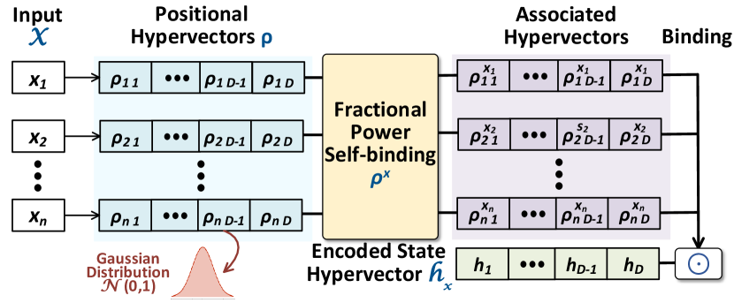
The encoding process in HDC is essentially mapping a vector of features to the high-dimensional space or hyperspace. HDC encoders need to maintain the relationship between input features in the hyperspace, e.g., two similar inputs are mapped to hypervectors with relatively larger cosine similarity [63]. For , we leverage the Fractional Power Encoding (FPE) to achieve a holographic reduced representation [8], i.e., symbols and their structured combinations can be represented uniformly in a hyperspace. In Fig. 2, we provide the outline of the HDC encoding process in .
We start by assuming a feature vector input of length : , and we view each feature in as a symbol to encode. The HDC encoder is pre-loaded with a series of positional hypervectors , each corresponding to one feature/position of the input feature. Elements in positional hypervectors are randomly sampled unitary phasors, i.e., where . Thus, the randomly sampled positional hypervectors are still near-orthogonal to each other in the hyperspace. Notice that although they are no longer bipolar hypervectors, binding and bundling operations mentioned in Section 2.4 still apply to them.
The difference in FPE lies in the way it associates features and their values. If we use regular binding defined in Section 2.4, two hypervectors, one for the feature and one for its value, will be combined using element-wise multiplication (e.g., ). This requires value quantization such that value hypervectors represent different discrete steps of feature values, which inevitably introduces information loss and cannot scale to data with large value ranges. FPE allows this to happen in a much finer granularity with fractional power self-binding [8]. Recall that binding results in a dissimilar hypervector, and thus we can encode integer feature values by repeatedly self-binding the feature positional hypervector. For example, we can encode as: . With FPE, a feature with floating number value is encoded similarly, e.g., is encoded by elementwise exponential . More generally, for the feature vector input , we have the encoding process as follows:
| (4) |
where we bind all encoded features together and stands for an matrix with each row being the vector. Notice that and similarity is real-valued, the similarity computation for hypervectors with FPE is defined as:
| (5) |
where is the complex conjugate and we normalize the real part of the dot product; this is also known as the Euclidean angle for complex vectors.
3.2 HDC Classification and Uncertainty Estimation with Naive Ensembles
BNNs with ensemble-based design have been leveraged for uncertainty-based AL since methods like MC-Dropout can estimate the model confidence via the variance in prediction [64]. On the other hand, HDC is also compatible with ensemble learning; we can train multiple HDC sub-models, each with its own HDC encoder and bootstrapped training set, i.e., bagging. During the inference, all sub-models will contribute to the prediction in a consensus-based way.
HDC Classification: We will now show procedures of HDC-based classification with ensemble learning. For a dataset with classes, the HDC model is comprised of class hypervectors , each has the same dimensionality as and . Class hypervectors can be trained through the bundling of all encoded training samples that share the same label, i.e., they are reduced representations for classes. HDC predicts by computing similarities of the encoded query hypervector and different class hypervectors and looking for the maximum.
Assume HDC sub-models , and the first sub-model will be trained with a data point with label . We first encode this sample to hypervector via equation 4 and then perform a similarity check with every class hypervector in model using equation 5. The prediction process for is shown below:
| (6) |
Then, class hypervectors will be updated according to how well the model predicts. More specifically, if the prediction is not correct (), the update process for sub-model is as the following:
| (7) |
| (8) |
where is the learning rate. The similarity values in the updates function as the feedback that dynamically controls the learning rate. For instance, a near 1 means that the class hypervector already contains the information in the query and only a slight update is needed as in equation 7; the wrong prediction may be the result of being incorrectly high, and therefore equation 8 will try to rectify. In addition, if the prediction is correct, then the HDC model is not updated. The process above happens separately for every sub-model during training based on bootstrapped sampling, and they are trained iteratively with batched samples.
Ensemble Inference & Uncertainty Estimation: As for the inference, every sub-model gives predictions on all testing data points. And for each data point, there is an array of predicted labels: . Regular ensemble inference uses voting to get the final prediction: . However, here we are interested in the predictive uncertainty, which can be estimated using entropy. To compute the entropy, we first approximate the probability of every predicted class label through:
| (9) |
where counts the number of sub-models that predict . Then the predictive entropy is computed as:
| (10) |
Intuitively, a higher entropy indicates that sub-models vote for different predictions, while a lower entropy close to zero infers that sub-models agree with each other.
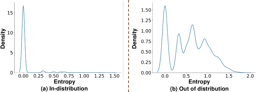
To qualitatively evaluate this estimation of model uncertainty, we apply HDC ensemble training using the MNIST dataset while testing on the NotMNIST [65] dataset, which is comprised of out-of-distribution (OOD) alphabet images with 10 classes and the same image size as MNIST. Since the ensemble model only knows handwritten digits from training, we expect the prediction probability to be closer to uniform during testing. In other words, each ensemble model will disagree with each other when evaluated on OOD samples, which results in a much larger predictive entropy.
In Fig. 3, we present the histogram of predictive entropy when testing the HDC naive ensemble with samples from both MNIST and NotMNIST datasets. For the in-distribution case, the histogram in Fig. 3(a) shows a high density around zero and indicates that ensemble sub-models agree with each other, i.e., lower uncertainty in prediction. As for the OOD case in Fig. 3(b), it is clear by comparison that the HDC naive ensemble now shows a higher level of uncertainty as larger entropy values show up in the histogram, indicating the disagreement between sub-models for some data points. However, the quality of this uncertainty estimation is lower than expected because the highest density still occurs at zero entropy values. This means that when deploying the naive ensemble design in practice, the HDC ensemble will frequently be over-confident about its prediction, and thereby unsuitable for uncertainty-based AL.
One possible reason why the HDC naive ensemble performs poorly is that HDC sub-models fail to understand the data space from diverse perspectives, which is crucial for fostering disagreement when facing unseen data points. In fact, due to the way model hypervectors are constructed, i.e., being the superposition of seen data, even with bootstrapping, these HDC sub-models are somewhat similar after training. Therefore, there is a high chance that sub-models will predict similar labels when they actually have low confidence.
3.3 HDC Prior Hypervectors
In previous HDC classification works, the model hypervectors are always initialized as zero vectors. Since these hypervectors are considered as the memory and prototype of data points of different classes, starting with zero values indicates no prior knowledge about the task or classes. Notice that this is different from DNNs with back-propagation training, as the zero initialization for neurons leads to uninformative gradients and poor learning results.
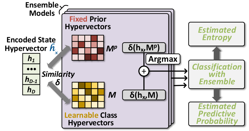
However, in , we enhance the naive design in Section 3.2 with HDC prior hypervectors that serve two purposes: first, they are non-zero initializations of HDC models; second, these hypervectors, as a whole, represent the prior model distribution or prior knowledge about a certain task. In Fig. 4, we give an overview of introducing prior hypervectors in HDC ensemble learning. We randomly sample these hypervectors with i.i.d. elements from the standard Gaussian distribution , and as a way of model initialization, we enable prior hypervectors for every sub-model in the HDC ensemble. We refer to them as , in contrast to regular HDC models .
As shown in Fig. 4, we perform two separate similarity checks in each sub-model; one is between the encoded data and HDC prior hypervectors and the other one is with model hypervectors . To make predictions, we combine these two sets of similarity values, e.g., for the first sub-model:
| (11) |
During the HDC model training, the prior hypervectors will not be updated and stay static and the model hypervectors follow slightly different update rules based on previous equations 7 and 8:
| (12) |
| (13) |
where is the sum of two similarity values. Introducing prior hypervectors to training and inference helps ensemble sub-models learn with diverse viewing angles and allows them to disagree with each other when uncertain.
We will name in Fig. 4 as isolated prior hypervectors, meaning their similarity with queries is computed separately. However, there is an obvious alternative to equation 11: , where the prior hypervectors are combined/bundled with model hypervectors before calculating the similarity. We compare the two different ways below:
| (14) |
| (15) |
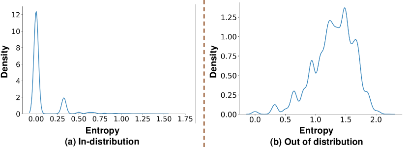
Fig. 5 compares the quality of uncertainty estimation between using isolated prior hypervectors and combining the prior with trainable models. With isolated prior hypervectors, in most cases, the HDC ensemble is able to reveal high uncertainty when predicting OOD test samples, showing an entropy value significantly larger than zero. However, when the prior hypervectors are combined into the model, the quality of uncertainty estimation is notably worse. The degradation may be attributed to the model hypervectors dominating the similarity computation. From equation 14 and 15, we observe that the difference is in the denominators: in the combined case, the norm is taken for the bundled hypervectors, whereas in the isolated case, the normalization happens separately, maintaining the influence of prior hypervectors on the overall similarity computation. More specifically, during HDC training, the model easily becomes much larger in norm (), diminishing the effect of and discouraging the diversity in sub-models.
In Algorithm 1, we present the pseudo-code for HDC ensemble learning with prior hypervectors, which is used in to aid the estimation of model uncertainty.
3.4 Computation Reuse and Neural Regeneration
In this section, we explore the opportunities for further improving the efficiency of HDC uncertainty estimation in . We will approach this via techniques such as a shared HDC encoder, encoded data reuse, similarity computation reuse, pre-normalization, and dynamic dimension regeneration.
Reuse Computation in HDC Ensemble: The key in ensemble learning is to construct multiple different sub-models; however, learning multiple models independently on every data point also leads to a several times higher cost. One difference between HDC-based and DNN-based ML models is that the HDC encoder is usually not updated once initialized. It is usually designed in advance since its main functionality is to generate high-dimensional and holographic representations for input data. With the analysis in previous sections, we also noticed that model (prior) hypervectors play a more important role in uncertainty estimation. Therefore, for HDC ensemble learning in , we propose to share the HDC encoder among all sub-models, meaning that they will use a uniform high-dimensional representation. There are at least two immediate benefits of sharing the encoder: (1) In AL, we can encode the training data pool only once in advance and reuse the encoded hypervectors for ensemble training and AL acquisition. They will significant amount of computation since both processes happen iteratively during the AL process. (2) Notice that both the HDC encoder and prior hypervectors are static, so, we can pre-compute and reuse their similarity values in equation 15. In practice, we can also pre-compute the normalization term of the similarity value.
HDC Neural Regeneration for Better Acquisition Efficiency: As operations in are centered around hypervectors, the computation cost scales with dimensionality. Thus, cutting down the dimensionality becomes a natural choice to further reduce the runtime cost of acquisition. We propose to leverage NeuralHD [44] to obtain even more lightweight HDC classification models. It introduces a mechanism to dynamically update the HDC encoder and is compatible with existing HDC classification algorithms including . Motivated by the regenerative ability of the brain, after a few epochs of HDC model update, NueralHD evaluates the significance of each dimension to the classification accuracy. The metric used here is the normalized variance across classes at each dimension of class hypervectors. NeuralHD updates the positional hypervectors of the HDC encoder by regenerating the dimensions that show low variance in class hypervectors. More specifically, we sample new values for those dimensions from standard Gaussian distribution again as in Section 3.1. This process makes NeuralHD more efficient in the utilization of hyperdimensions and maintains high accuracy with much smaller HDC models (i.e., much fewer hyperdimensions). Due to the limited space, for more details regarding this algorithm, we refer readers to the original paper [44]. For our design, with NeuralHD regeneration, we reduce the hypervector dimensionality in by up to 50%.
4 HDC-based Active Learning
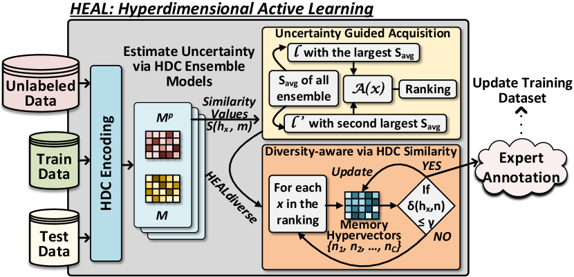
In Fig. 6, we present the overview of , our proposed HDC-based AL framework. It has three main components: HDC ensemble learning for uncertainty estimation (covered in the previous Section 3), uncertainty-based acquisition, and HDC diversity-enhanced AL. In this section, we will focus on the latter two.
4.1 Uncertainty-based Acquisition via Hypervector Similarity
It is common for AL techniques to leverage probabilities in the acquisition function because DNNs usually add a softmax layer to normalize logits and get probability values in the range of 0 to 1. However, HDC does not give outputs interpretable as probabilities nor does it learn based on cross-entropy loss. This means that adding an extra softmax layer will not give informative predictive probabilities. Instead of using softmax, in equation 9, we estimate the predictive probability from predictions of ensemble sub-models. Although we have shown that it is quite useful for qualitative analysis, this is inevitably a coarse approximation and will limit its usage in uncertainty-based AL.
With no access to predictive probabilities, prior AL techniques like confidence and entropy sampling are unsuitable for HDC. However, we noticed that the margin sampling, although based on probabilities in the original design, can be adapted for HDC. It captures model uncertainty through the margin between the top two predictions, which generalizes beyond probability values. In , we propose to directly utilize the similarity values from equation 15 and compute the prediction margin in the AL acquisition function:
| (16) |
The value of becomes larger when the similarity with gets closer to the one with , i.e., higher uncertainty about . We apply ensemble model averaging for similarity values; is the predicted label with the highest average similarity values and is the one with the second highest values.
| (17) |
where represents the model(prior) hypervectors of class corresponding to the -th sub-model. In every acquisition step, we sample a batch of data points from , which rank top- in the values of .
HDC ensemble with prior hypervectors plays a key role in the acquisition process. After training, each sub-model can be confident about its prediction, giving high similarity values for the predicted class. However, sub-models will predict different labels for data points that the ensemble model as a whole is uncertain about. With ensemble model averaging in equation 17, the similarity value for a particular class is much lower due to the disagreement, and the margin sampling in equation 16 will capture the narrowed gap between top-2 predictions.
4.2 Diversity Metric via Hypervector Memorization
One common challenge in uncertainty-based AL is that the algorithm tends to select similar samples in batch acquisition. Notice that during batch acquisition, the model is not updated immediately until a full batch of data points is annotated. Therefore, a top- ranking will repeatedly select helpful data points that contain duplicate information. As we mentioned in Section 2.3, DNN-based AL methods cope with this problem via joint mutual information, representative sampling, and data mining algorithms, although with significant acquisition overheads due to these added components.
In this section, we propose an efficient diversity metric that helps acquire not only informative but also diverse data points, without introducing costly computations as in prior DNN-based methods. We utilize lightweight HDC operations and leverage the intrinsic memorization capability of hypervectors to achieve diverse acquisition. We notice that the requirement for diversity can be achieved by checking the similarity between the candidate data point and existing points in the current batch. In other words, hypervector similarity checks can be a strong tool for filtering out duplicate data points. This diversity metric can be seamlessly included in since the dataset has already been encoded to hypervector representations.
As shown in Fig. 6, instead of computing pair-wise similarity, we consider the acquired data points altogether by constructing a memorization hypervector for each class . These hypervectors memorize and categorize the acquired data points according to the pseudo label , i.e., the label predicted by all HDC sub-models via voting. They are initialized with all-zero vectors. To begin with, we perform inference on the unlabeled dataset and rank it via the acquisition function to prioritize the data points for which the model has lower confidence. The first acquired data point (i.e., the one with the largest value of ) will be automatically added to the batch. We update the memory hypervector that corresponds to the pseudo label: . For the next candidate data point that ranked second, if it has the same pseudo label as , we will check its similarity with the memorization hypervector: . We only acquire this sample when it shows low similarity values and discard it if otherwise. In our implementation, we use a similarity threshold . If its prediction leads to a yet empty memory hypervector, it will be acquired directly. We will repeat this process until the batch has been filled with acquired data points. For the next step of batch acquisition, the memory hypervectors are re-initialized.
We present the pseudo-code for in Algorithm 2. Before the acquisition process, we first pre-encode and pre-compute similarities with prior hypervectors as mentioned in Section 3.4. Then in each acquisition step , we annotate the acquired data points to the training dataset, remove them from , and then train the ensemble model on the new training set.
Datasets # Train Samples # Test Samples # Features # Classes ISOLET [66] 5847 1950 617 26 UCIHAR [67] 5825 1942 561 12 DSADS [68] 6840 2280 405 19 PAMAP [69] 5484 1828 243 19
5 Experiments
5.1 Experimental Settings
To evaluate the performance of , we compare it against several existing AL algorithms that are widely applied, including traditional methods that are based on simple measures, and modern methods that are either non-Bayesian or Bayesian in terms of how uncertainty is estimated. Our baselines also include AL algorithms that explicitly consider diversity in acquisition. The following is a list of the baseline algorithms used in comparison.
-
1.
Rand: A naive design (i.e., non-AL) that randomly acquires unlabeled samples for expert annotation.
-
2.
Conf (Confidence Sampling): uses simple model confidence as the sign for uncertainty [20]. The acquisition starts with the sample with the lowest predicted class probability.
-
3.
Marg (Margin Sampling): An uncertainty-based algorithm, whose uncertainty metric is built upon the probability difference between the top-2 predicted classes [35]. The sample with the smallest margin will be selected first for annotation. Margin sampling can be enhanced by BNNs for better uncertainty estimation.
-
(a)
Marg_de: It uses Deep Ensemble as the BNN backbone.
-
(b)
Marg_dropout: uses MC-Dropout as the BNN backbone.
-
(a)
-
4.
ALBL: A hybrid AL method that aims at the balance between uncertainty-based (Conf) and diversity-based (Coreset) AL algorithms via bandit-style selection [17].
-
5.
BADGE: An intelligent hybrid method that uses gradient information in the DNN classifier to incorporate both predictive uncertainty and sample diversity into acquisition [16].
-
6.
BatchBALD: An information-theoretic AL method that identifies the most informative samples based on estimated information gain, computed via Bayesian models [19]. The metric used considers both model uncertainty and diversity of the acquired batch.
As for our proposed , since many of its components are optional during practical implementations, we evaluated it with the following different settings:
-
•
: the bare bone of our uncertainty-based AL framework using HDC ensemble with prior hypervectors.
-
•
: enhanced by hyperdimension regeneration for a more lightweight model and faster acquisition.
-
•
: enhanced by HDC memory hypervectors for diversity-aware batch acquisition.
Our AL evaluation follows the batch-mode setup; for all algorithms, it starts with 20 initial labeled training samples (), and the acquisition batch size for each AL step ranges from 20 to 200. As for the model backbone, similar to BatchBALD, we select the multilayer perception (MLP) model for all DNN/BNN-based AL on all datasets; it has two hidden layers and each layer has 256 neurons. The models are trained on Pytorch using cross-entropy loss and the Adam optimizer. For and , we use hypervectors with ; and , as we mentioned before, uses . For all algorithms, we train the classifier from scratch at every step of acquisition until the training accuracy hits 99%. All experiments are repeated five times and averaged.
We showcase our proposed AL frameworks on four different open datasets, as shown in Table 1. The first dataset is a speech recognition dataset and the rest three are for human activity recognition tasks. In practice, human activity recognition mainly involves on-body multi-sensor data analysis, where collecting labeled data for diverse user groups takes a significant amount of effort. Our experiments aim to show the effectiveness of AL algorithms, especially , on saving annotation costs in similar tasks. Notice that the DSADS and PAMAP datasets undergo a widely applied data preprocessing as described in [70].
5.2 Active Learning Performance and Efficiency
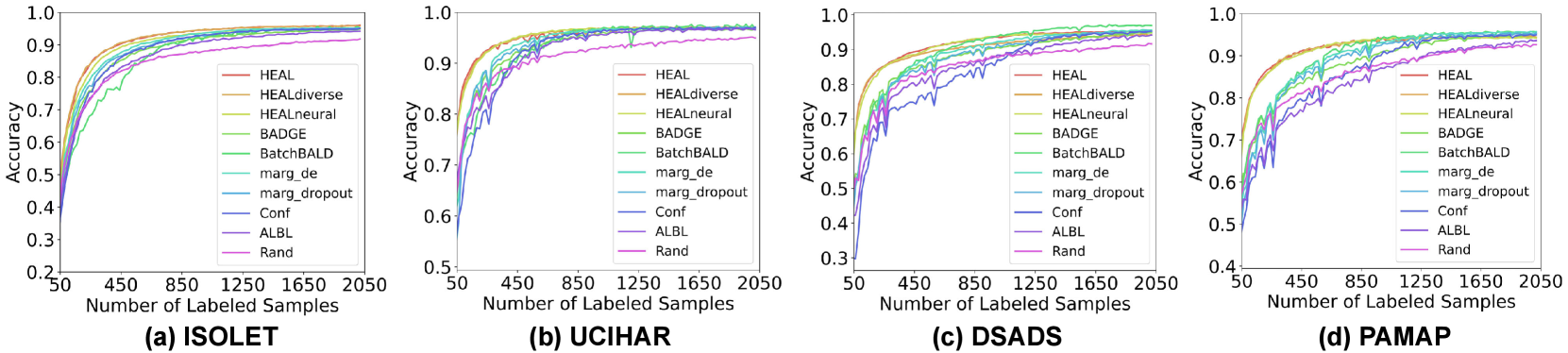
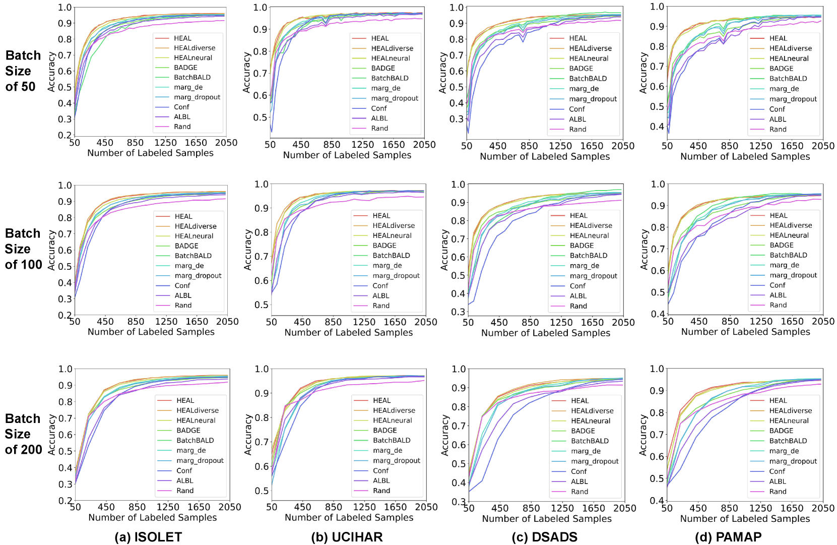
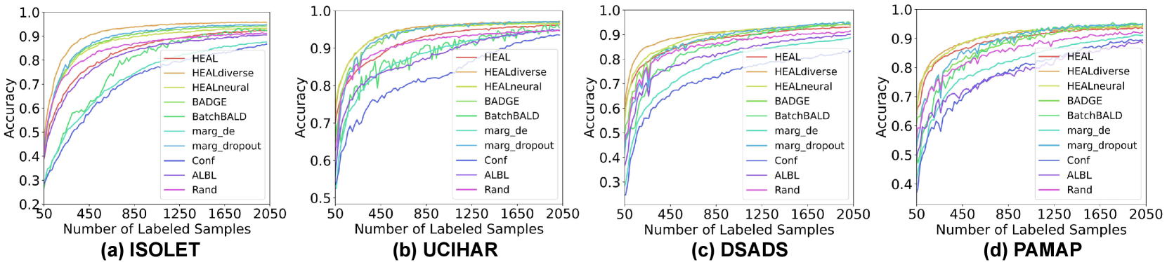
The learning curve is an intuitive way to evaluate the effectiveness of AL algorithms, which record the testing accuracy at each step of acquisition with an increasing number of labeled samples. In Fig. 7, we show the averaged testing accuracy of five runs for all four datasets and different AL algorithms. The batch size of acquisition is . In Fig. 8, we present learning curves with other batch sizes (). Firstly, we observe that all AL algorithms eventually outperform random acquisition by a noticeable gap. Most AL algorithms help reach model convergence much faster than the case without AL. As for the performance of methods with different configurations, they often achieve significantly higher testing accuracy than other baselines during the first half of the curve, i.e., with less than 1000 labeled samples. When closer to model convergence, enhanced HDC classifier is comparable to hybrid AL methods including BADGE and BatchBALD. Albeit using similar acquisition metrics as margin sampling, achieves better AL quality, thanks to the optimal combination of HDC’s intrinsic learning efficiency and our uniquely developed uncertainty estimation approach for HDC-based classifiers. For more comparison between different variants of margin sampling and , please refer to Fig. 14. For illustrations of HDC inherent learning efficiency and its comparison with , please refer to Fig. 15.
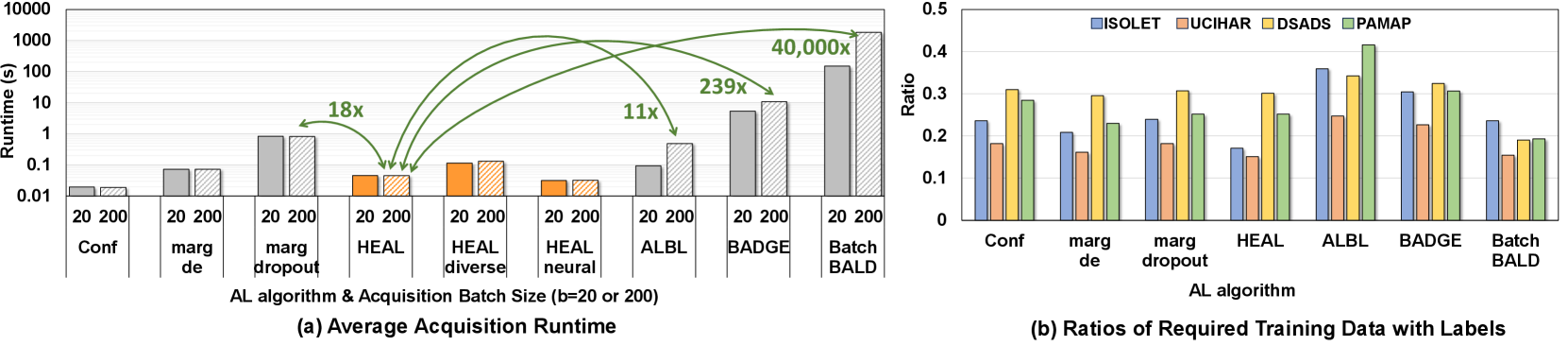
To illustrate the efficiency of our AL framework, we collect the acquisition runtime for most algorithms (including ) using Intel Core i7-12700 CPU; except for BatchBALD, which is not efficient and scalable on CPU platforms, we use NVIDIA RTX 4090 GPU instead. In Fig. 9(a), we compare the average acquisition runtime of each AL method with two different batch size settings. As highlighted in this figure, and its variants have notably faster acquisition compared to most baselines. When , the speedups of over marginal sampling with dropout, ALBL, BADGE, and BatchBALD are 18, 11, 239, and more than 40000, respectively. Confidence sampling is the fastest in acquisition due to its non-Bayesian uncertainty estimation. However, this naive estimation leads to its sub-optimal performance in AL. With the help of NeuralHD, is about 45% faster than regular in acquisition. Due to the diversity-aware acquisition module, there is a relatively small overhead in . In Section 5.3, we will present the benefits brought by this extra module. In Fig. 9 (b), we show the size of the labeled training dataset needed for each AL method to achieve 99% of the accuracy obtained with the full dataset. This metric represents how much annotation effort can be saved with AL. The figure shows that is on average better than most baselines except the information-theoretic BatchBALD which comes at a huge cost. Note that the acquisition in BatchBALD is significantly slower than others even if it is the only method run on a powerful GPU. This is because BatchBALD suffers from the combinatorial explosion in its estimation of joint distributions [19].
5.3 AL in datasets with duplicated samples
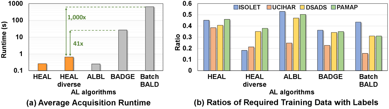
As we mentioned in Section 4.2, datasets with a large number of similar samples pose challenges to many existing AL algorithms. Therefore, in this section, we ramp up the difficulty and evaluate these AL methods on specially modified datasets. For each of the previously tested datasets, we copy the training dataset four times, meaning that each unique sample now has five duplicates. We then repeat the evaluations in Section 5.2 and record the learning curves in Fig. 10. As expected, AL methods without effective diversity metrics such as confidence sampling and marg_de suffer from significant degradation in AL performance. In addition, the performance of ALBL over confidence sampling hints at the benefit of filtering out duplicate samples during acquisition. Nevertheless, many AL algorithms are showing acquisition quality worse than random selection. In contrast, methods like and BADGE still maintain high acquisition efficiency with giving the highest testing accuracy in the first half of the learning curve. Methods including BADGE and BatchBALD are also among the best performing AL methods during the second half, however, their acquisition costs are orders of magnitude larger. Also interestingly, we observe that methods that rely solely on ensemble generally perform poorly, as their sub-models are prone to be similar due to training on an overflow of duplicated samples and thereby compromise their uncertainty estimation. Fig. 11(a) shows that is 41 (1000) faster than BADGE (BatchBALD) in terms of the average acquisition runtime. Fig. 11(b) shows that is among the best performing AL methods for all datasets and significantly outperforms the regular design.
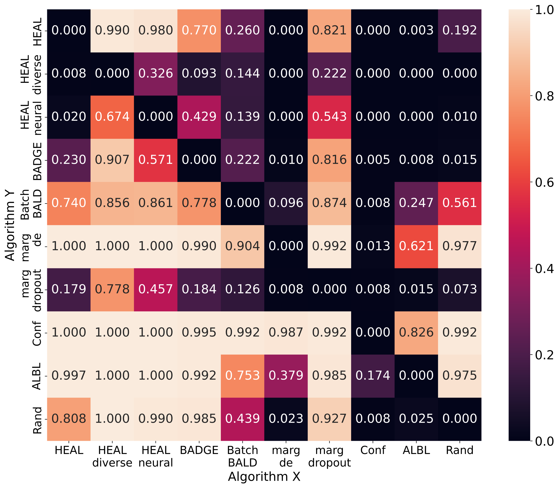
5.4 Pair-wise comparison
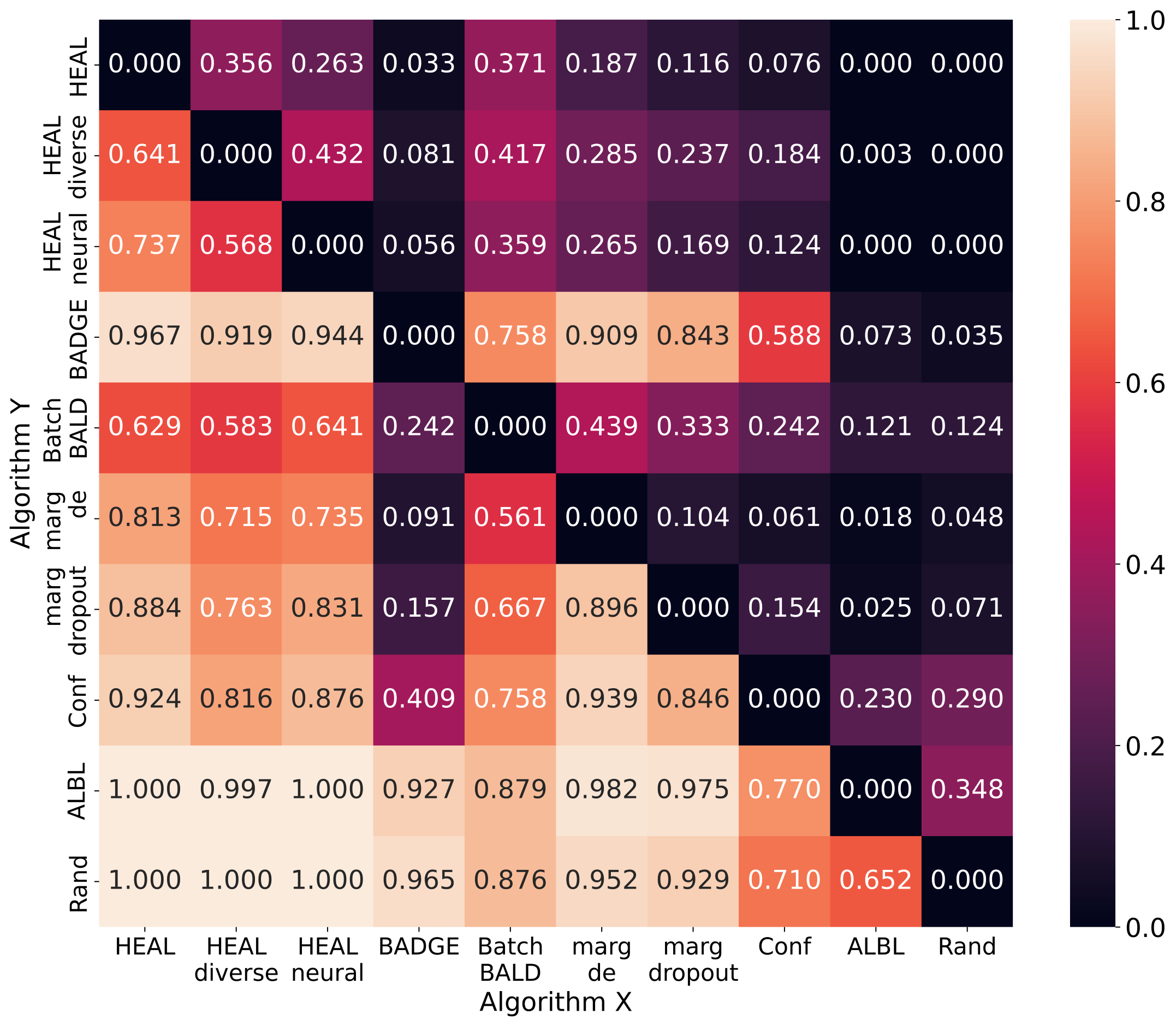
To better compare different AL methods comprehensively, we apply a pair-wise comparison method proposed in [16]. Every time algorithm X beats algorithm Y in terms of testing accuracy, the latter accumulates a certain amount of penalty. We normalize the values to . Fig. 12 is the pair-wise comparison averaged on datasets without duplicate samples, and Fig. 13 is averaged on datasets with duplicate samples. A better-performing AL method shows more small values (i.e., dark color) in a row, e.g., outperforms in Fig. 12 and in Fig. 13.
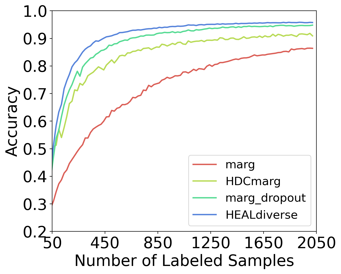
5.5 Benefits of using advanced uncertainty estimation in AL
In this section, we illustrate the benefits of designing non-trivial uncertainty estimation techniques for AL by comparing methods with or without these techniques. In Fig. 14, ’marg’ stands for the basic margin sampling without using any BNNs, and ’HDCmarg’ refers to simple HDC similarity-based margin sampling without HDC ensemble models with prior hypervectors. In general, and margin sampling with MC-dropout significantly outperform their naive versions.
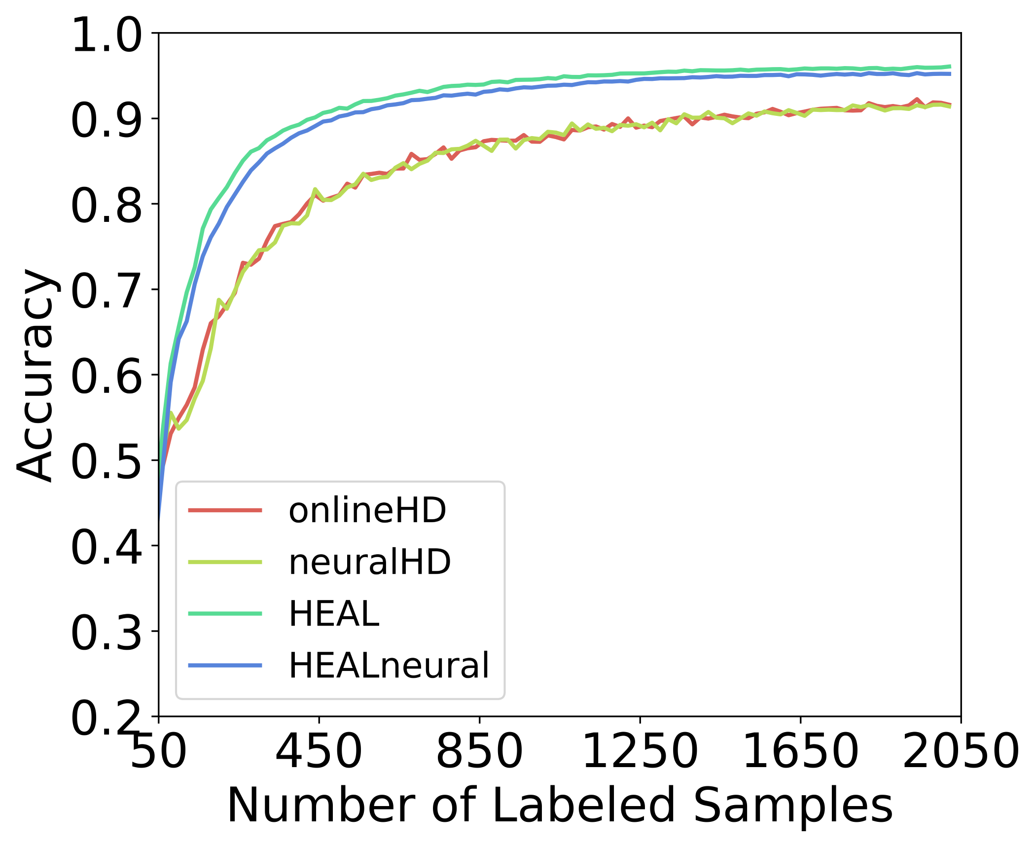
5.6 Comparison against HDC classifiers without AL
Prior HDC arts such as OnlineHD and NeuralHD are known for their better learning efficiency, which mainly comes from the brain-inspired hypervector representation and operations. In Fig. 15, we compare the and to their classifier backbones in terms of the learning curve. As for OnlineHD and NeuralHD, due to the lack of an AL framework, they will select random samples for annotation. The clear gap in the figure highlights the efficacy of the and underscores the advantages of integrating the existing capabilities of HDC with a tailored AL framework to further enhance learning efficiency.
6 Conclusion
We introduced Hyperdimensional Efficient Active Learning (), an AL framework specifically designed for HDC classification. distinguishes itself by utilizing HDC-centered uncertainty and diversity-aware strategies to annotate unlabeled data efficiently. Our approach demonstrates its strength over traditional AL methods, achieving higher data efficiency and notable speedups in acquisition.
References
- [1] T. Brown, B. Mann, N. Ryder, M. Subbiah, J. D. Kaplan, P. Dhariwal, A. Neelakantan, P. Shyam, G. Sastry, A. Askell, et al., “Language models are few-shot learners,” Advances in neural information processing systems, vol. 33, pp. 1877–1901, 2020.
- [2] H. Touvron, L. Martin, K. Stone, P. Albert, A. Almahairi, Y. Babaei, N. Bashlykov, S. Batra, P. Bhargava, S. Bhosale, et al., “Llama 2: Open foundation and fine-tuned chat models,” arXiv preprint arXiv:2307.09288, 2023.
- [3] P. Kanerva, “Hyperdimensional computing: An introduction to computing in distributed representation with high-dimensional random vectors,” Cognitive computation, vol. 1, pp. 139–159, 2009.
- [4] A. Hernandez-Cane, N. Matsumoto, E. Ping, and M. Imani, “Onlinehd: Robust, efficient, and single-pass online learning using hyperdimensional system,” in 2021 Design, Automation & Test in Europe Conference & Exhibition (DATE), pp. 56–61, IEEE, 2021.
- [5] P. Poduval, H. Alimohamadi, A. Zakeri, F. Imani, M. H. Najafi, T. Givargis, and M. Imani, “Graphd: Graph-based hyperdimensional memorization for brain-like cognitive learning,” Frontiers in Neuroscience, vol. 16, p. 757125, 2022.
- [6] H. E. Barkam, S. Yun, P. R. Genssler, Z. Zou, C.-K. Liu, H. Amrouch, and M. Imani, “Hdgim: Hyperdimensional genome sequence matching on unreliable highly scaled fefet,” in 2023 Design, Automation & Test in Europe Conference & Exhibition (DATE), pp. 1–6, IEEE, 2023.
- [7] B. Babadi and H. Sompolinsky, “Sparseness and expansion in sensory representations,” Neuron, vol. 83, no. 5, pp. 1213–1226, 2014.
- [8] T. A. Plate, “Holographic reduced representations,” IEEE Transactions on Neural networks, vol. 6, no. 3, pp. 623–641, 1995.
- [9] E. P. Frady, D. Kleyko, C. J. Kymn, B. A. Olshausen, and F. T. Sommer, “Computing on functions using randomized vector representations (in brief),” in Proceedings of the 2022 Annual Neuro-Inspired Computational Elements Conference, pp. 115–122, 2022.
- [10] E. Camina and F. Güell, “The neuroanatomical, neurophysiological and psychological basis of memory: Current models and their origins,” Frontiers in pharmacology, vol. 8, p. 438, 2017.
- [11] H. Chen, A. Zakeri, F. Wen, H. E. Barkam, and M. Imani, “Hypergraf: Hyperdimensional graph-based reasoning acceleration on fpga,” in 2023 33rd International Conference on Field-Programmable Logic and Applications (FPL), pp. 34–41, IEEE, 2023.
- [12] H. Chen, M. Issa, Y. Ni, and M. Imani, “Darl: Distributed reconfigurable accelerator for hyperdimensional reinforcement learning,” in Proceedings of the 41st IEEE/ACM International Conference on Computer-Aided Design, pp. 1–9, 2022.
- [13] Y. Ni, Y. Kim, T. Rosing, and M. Imani, “Algorithm-hardware co-design for efficient brain-inspired hyperdimensional learning on edge,” in 2022 Design, Automation & Test in Europe Conference & Exhibition (DATE), pp. 292–297, IEEE, 2022.
- [14] Y. Ni, M. Issa, D. Abraham, M. Imani, X. Yin, and M. Imani, “Hdpg: hyperdimensional policy-based reinforcement learning for continuous control,” in Proceedings of the 59th ACM/IEEE Design Automation Conference, pp. 1141–1146, 2022.
- [15] N. Houlsby, F. Huszár, Z. Ghahramani, and M. Lengyel, “Bayesian active learning for classification and preference learning,” arXiv preprint arXiv:1112.5745, 2011.
- [16] J. T. Ash, C. Zhang, A. Krishnamurthy, J. Langford, and A. Agarwal, “Deep batch active learning by diverse, uncertain gradient lower bounds,” arXiv preprint arXiv:1906.03671, 2019.
- [17] W.-N. Hsu and H.-T. Lin, “Active learning by learning,” in Proceedings of the AAAI Conference on Artificial Intelligence, vol. 29, 2015.
- [18] O. Sener and S. Savarese, “Active learning for convolutional neural networks: A core-set approach,” arXiv preprint arXiv:1708.00489, 2017.
- [19] A. Kirsch, J. Van Amersfoort, and Y. Gal, “Batchbald: Efficient and diverse batch acquisition for deep bayesian active learning,” Advances in neural information processing systems, vol. 32, 2019.
- [20] D. Wang and Y. Shang, “A new active labeling method for deep learning,” in 2014 International joint conference on neural networks (IJCNN), pp. 112–119, IEEE, 2014.
- [21] A. Graves, “Practical variational inference for neural networks,” Advances in neural information processing systems, vol. 24, 2011.
- [22] M. D. Hoffman, D. M. Blei, C. Wang, and J. Paisley, “Stochastic variational inference,” Journal of Machine Learning Research, 2013.
- [23] C. Blundell, J. Cornebise, K. Kavukcuoglu, and D. Wierstra, “Weight uncertainty in neural network,” in International conference on machine learning, pp. 1613–1622, PMLR, 2015.
- [24] Y. Gal and Z. Ghahramani, “Dropout as a bayesian approximation: Representing model uncertainty in deep learning,” in international conference on machine learning, pp. 1050–1059, PMLR, 2016.
- [25] R. M. Neal, Bayesian learning for neural networks, vol. 118. Springer Science & Business Media, 2012.
- [26] G. E. Hinton and D. Van Camp, “Keeping the neural networks simple by minimizing the description length of the weights,” in Proceedings of the sixth annual conference on Computational learning theory, pp. 5–13, 1993.
- [27] D. Barber and C. M. Bishop, “Ensemble learning in bayesian neural networks,” Nato ASI Series F Computer and Systems Sciences, vol. 168, pp. 215–238, 1998.
- [28] M. I. Jordan, Z. Ghahramani, T. S. Jaakkola, and L. K. Saul, “An introduction to variational methods for graphical models,” Machine learning, vol. 37, pp. 183–233, 1999.
- [29] D. J. MacKay, “Probable networks and plausible predictions-a review of practical bayesian methods for supervised neural networks,” Network: computation in neural systems, vol. 6, no. 3, p. 469, 1995.
- [30] B. Lakshminarayanan, A. Pritzel, and C. Blundell, “Simple and scalable predictive uncertainty estimation using deep ensembles,” Advances in neural information processing systems, vol. 30, 2017.
- [31] F. K. Gustafsson, M. Danelljan, and T. B. Schon, “Evaluating scalable bayesian deep learning methods for robust computer vision,” in Proceedings of the IEEE/CVF conference on computer vision and pattern recognition workshops, pp. 318–319, 2020.
- [32] Y. Ovadia, E. Fertig, J. Ren, Z. Nado, D. Sculley, S. Nowozin, J. Dillon, B. Lakshminarayanan, and J. Snoek, “Can you trust your model’s uncertainty? evaluating predictive uncertainty under dataset shift,” Advances in neural information processing systems, vol. 32, 2019.
- [33] V. Růžička, S. D’Aronco, J. D. Wegner, and K. Schindler, “Deep active learning in remote sensing for data efficient change detection,” arXiv preprint arXiv:2008.11201, 2020.
- [34] B. Liu and V. Ferrari, “Active learning for human pose estimation,” in Proceedings of the IEEE International Conference on Computer Vision, pp. 4363–4372, 2017.
- [35] D. Roth and K. Small, “Margin-based active learning for structured output spaces,” in Machine Learning: ECML 2006: 17th European Conference on Machine Learning Berlin, Germany, September 18-22, 2006 Proceedings 17, pp. 413–424, Springer, 2006.
- [36] X. Lv, F. Duan, J.-J. Jiang, X. Fu, and L. Gan, “Deep active learning for surface defect detection,” Sensors, vol. 20, no. 6, p. 1650, 2020.
- [37] A. J. Joshi, F. Porikli, and N. Papanikolopoulos, “Multi-class active learning for image classification,” in 2009 ieee conference on computer vision and pattern recognition, pp. 2372–2379, IEEE, 2009.
- [38] J. M. Hernández-Lobato and R. Adams, “Probabilistic backpropagation for scalable learning of bayesian neural networks,” in International conference on machine learning, pp. 1861–1869, PMLR, 2015.
- [39] Y. Geifman and R. El-Yaniv, “Deep active learning over the long tail,” arXiv preprint arXiv:1711.00941, 2017.
- [40] S.-J. Huang, R. Jin, and Z.-H. Zhou, “Active learning by querying informative and representative examples,” Advances in neural information processing systems, vol. 23, 2010.
- [41] D. Arthur and S. Vassilvitskii, “K-means++ the advantages of careful seeding,” in Proceedings of the eighteenth annual ACM-SIAM symposium on Discrete algorithms, pp. 1027–1035, 2007.
- [42] P. Poduval, Y. Ni, Y. Kim, K. Ni, R. Kumar, R. Cammarota, and M. Imani, “Adaptive neural recovery for highly robust brain-like representation,” in Proceedings of the 59th ACM/IEEE Design Automation Conference, pp. 367–372, 2022.
- [43] M. Heddes, I. Nunes, P. Vergés, D. Kleyko, D. Abraham, T. Givargis, A. Nicolau, and A. Veidenbaum, “Torchhd: An open source python library to support research on hyperdimensional computing and vector symbolic architectures,” Journal of Machine Learning Research, vol. 24, no. 255, pp. 1–10, 2023.
- [44] Z. Zou, Y. Kim, F. Imani, H. Alimohamadi, R. Cammarota, and M. Imani, “Scalable edge-based hyperdimensional learning system with brain-like neural adaptation,” in Proceedings of the International Conference for High Performance Computing, Networking, Storage and Analysis, pp. 1–15, 2021.
- [45] S. Gupta, B. Khaleghi, S. Salamat, J. Morris, R. Ramkumar, J. Yu, A. Tiwari, J. Kang, M. Imani, B. Aksanli, et al., “Store-n-learn: Classification and clustering with hyperdimensional computing across flash hierarchy,” ACM Transactions on Embedded Computing Systems (TECS), vol. 21, no. 3, pp. 1–25, 2022.
- [46] M. Imani, Y. Kim, T. Worley, S. Gupta, and T. Rosing, “Hdcluster: An accurate clustering using brain-inspired high-dimensional computing,” in 2019 Design, Automation & Test in Europe Conference & Exhibition (DATE), pp. 1591–1594, IEEE, 2019.
- [47] A. Hernández-Cano, C. Zhuo, X. Yin, and M. Imani, “Reghd: Robust and efficient regression in hyper-dimensional learning system,” in 2021 58th ACM/IEEE Design Automation Conference (DAC), pp. 7–12, IEEE, 2021.
- [48] Y. Ni, D. Abraham, M. Issa, Y. Kim, P. Mercati, and M. Imani, “Efficient off-policy reinforcement learning via brain-inspired computing,” in Proceedings of the Great Lakes Symposium on VLSI 2023, pp. 449–453, 2023.
- [49] M. Issa, S. Shahhosseini, Y. Ni, T. Hu, D. Abraham, A. M. Rahmani, N. Dutt, and M. Imani, “Hyperdimensional hybrid learning on end-edge-cloud networks,” in 2022 IEEE 40th International Conference on Computer Design (ICCD), pp. 652–655, IEEE, 2022.
- [50] Z. Zou, H. Chen, P. Poduval, Y. Kim, M. Imani, E. Sadredini, R. Cammarota, and M. Imani, “Biohd: an efficient genome sequence search platform using hyperdimensional memorization,” in Proceedings of the 49th Annual International Symposium on Computer Architecture, pp. 656–669, 2022.
- [51] H. Chen, M. H. Najafi, E. Sadredini, and M. Imani, “Full stack parallel online hyperdimensional regression on fpga,” in 2022 IEEE 40th International Conference on Computer Design (ICCD), pp. 517–524, IEEE, 2022.
- [52] W. Xu, V. Swaminathan, S. Pinge, S. Fuhrman, and T. Rosing, “Hypermetric: Robust hyperdimensional computing on error-prone memories using metric learning,” in 2023 IEEE 41st International Conference on Computer Design (ICCD), pp. 243–246, IEEE, 2023.
- [53] H. E. Barkam, S. Yun, H. Chen, P. Gensler, A. Mema, A. Ding, G. Michelogiannakis, H. Amrouch, and M. Imani, “Reliable hyperdimensional reasoning on unreliable emerging technologies,” in 2023 IEEE/ACM International Conference On Computer Aided Design (ICCAD), pp. 1–9, IEEE, 2023.
- [54] U. Pale, T. Teijeiro, S. Rheims, P. Ryvlin, and D. Atienza, “Combining general and personal models for epilepsy detection with hyperdimensional computing,” Artificial Intelligence in Medicine, vol. 148, p. 102754, 2024.
- [55] S. Shahhosseini, Y. Ni, E. Kasaeyan Naeini, M. Imani, A. M. Rahmani, and N. Dutt, “Flexible and personalized learning for wearable health applications using hyperdimensional computing,” in Proceedings of the Great Lakes Symposium on VLSI 2022, pp. 357–360, 2022.
- [56] Y. Ni, N. Lesica, F.-G. Zeng, and M. Imani, “Neurally-inspired hyperdimensional classification for efficient and robust biosignal processing,” in Proceedings of the 41st IEEE/ACM International Conference on Computer-Aided Design, pp. 1–9, 2022.
- [57] A. Rahimi, A. Tchouprina, P. Kanerva, J. d. R. Millán, and J. M. Rabaey, “Hyperdimensional computing for blind and one-shot classification of eeg error-related potentials,” Mobile Networks and Applications, vol. 25, pp. 1958–1969, 2020.
- [58] A. Burrello, K. Schindler, L. Benini, and A. Rahimi, “One-shot learning for ieeg seizure detection using end-to-end binary operations: Local binary patterns with hyperdimensional computing,” in 2018 IEEE Biomedical Circuits and Systems Conference (BioCAS), pp. 1–4, IEEE, 2018.
- [59] M. Imani, A. Zakeri, H. Chen, T. Kim, P. Poduval, H. Lee, Y. Kim, E. Sadredini, and F. Imani, “Neural computation for robust and holographic face detection,” in Proceedings of the 59th ACM/IEEE Design Automation Conference, pp. 31–36, 2022.
- [60] R. Thapa, B. Lamichhane, D. Ma, and X. Jiao, “Spamhd: Memory-efficient text spam detection using brain-inspired hyperdimensional computing,” in 2021 IEEE Computer Society Annual Symposium on VLSI (ISVLSI), pp. 84–89, IEEE, 2021.
- [61] K. Shridhar, H. Jain, A. Agarwal, and D. Kleyko, “End to end binarized neural networks for text classification,” in Proceedings of SustaiNLP: Workshop on Simple and Efficient Natural Language Processing, pp. 29–34, 2020.
- [62] Y. Ni, H. Chen, P. Poduval, Z. Zou, P. Mercati, and M. Imani, “Brain-inspired trustworthy hyperdimensional computing with efficient uncertainty quantification,” in 2023 IEEE/ACM International Conference on Computer Aided Design (ICCAD), pp. 01–09, IEEE, 2023.
- [63] S. Aygun, M. S. Moghadam, M. H. Najafi, and M. Imani, “Learning from hypervectors: A survey on hypervector encoding,” arXiv preprint arXiv:2308.00685, 2023.
- [64] Y. Gal, R. Islam, and Z. Ghahramani, “Deep bayesian active learning with image data,” in International conference on machine learning, pp. 1183–1192, PMLR, 2017.
- [65] Y. Bulatov, “Notmnist dataset,” Technical report[Online]. Available: http://yaroslavvb.blogspot.it/2011/09/notmnist-dataset.html, 2011.
- [66] D. Dua and C. Graff, “Isolet dataset, UCI machine learning repository,” 2017.
- [67] D. Anguita, A. Ghio, L. Oneto, X. Parra, J. L. Reyes-Ortiz, et al., “A public domain dataset for human activity recognition using smartphones.,” in Esann, vol. 3, p. 3, 2013.
- [68] B. Barshan and M. C. Yüksek, “Recognizing daily and sports activities in two open source machine learning environments using body-worn sensor units,” The Computer Journal, vol. 57, no. 11, pp. 1649–1667, 2014.
- [69] A. Reiss and D. Stricker, “Introducing a new benchmarked dataset for activity monitoring,” in 2012 16th international symposium on wearable computers, pp. 108–109, IEEE, 2012.
- [70] J. Wang, Y. Chen, L. Hu, X. Peng, and S. Y. Philip, “Stratified transfer learning for cross-domain activity recognition,” in 2018 IEEE international conference on pervasive computing and communications (PerCom), pp. 1–10, IEEE, 2018.