HEAT EQUATION ON THE HYPERGRAPH CONTAINING VERTICES WITH GIVEN DATA

Takeshi Fukao, Masahiro Ikeda, Shun Uchida^†^†Corresponding author: shunuchida@oita-u.ac.jp

Abstract

This paper is concerned with the Cauchy problem of a multivalued ordinary differential equation governed by the hypergraph Laplacian, which describes the diffusion of “heat” or “particles” on the vertices of hypergraph. We consider the case where the heat on several vertices are manipulated internally by the observer, namely, are fixed by some given functions. This situation can be reduced to a nonlinear evolution equation associated with a time-dependent subdifferential operator, whose solvability has been investigated in numerous previous researches. In this paper, however, we give an alternative proof of the solvability in order to avoid some complicated calculations arising from the chain rule for the time-dependent subdifferential. As for results which cannot be assured by the known abstract theory, we also discuss the continuous dependence of solution on the given data and the time-global behavior of solution.

^†^† 2020 Mathematics Subject Classification: Primary 34G25; Secondary 05C65, 47J30, 47J35. ^†^† Keywords: Hypergraph, hypergraph Laplacian, subdifferential, nonlinear evolution equation, constraint problem.

1 Introduction

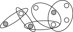
Let $V=\{v_{1},\ldots,v_{n},v_{n+1},\ldots,v_{n+m}\}$ be a finite set, $E\subset 2^{V}$ be a family of subsets consisting of two or more elements of $V$ , and $w:E\to(0,\infty)$ . The triplet $G=(V,E,w)$ , which is called hypergraph, can be interpreted as a model of a network structure in which vertices $v_{1},\ldots,v_{n+m}\in V$ are connected by each hyperedge $e\in E$ (see Fig. 1).

Refer to caption — Figure 1: When # $e=2$ for every $e\in E$ , each edge $e\in E$ can be regarded as a segment connecting two vertices (left figure, called usual graph). Hypergraph is a generalization of usual graph which represents the connection and grouping of multiple members (right figure).

In order to investigate the structure of network represented by a hypergraph, Yoshida [16] introduced a nonlinear set-valued operator on $\mathbb{R}^{V}$ (the family of mappings $x:V\to\mathbb{R}$ ) as follows. Define $f_{e}(x):=\max_{u,v\in e}(x(u)-x(v))$ with respect to each $e\in E$ and

(1)

\varphi_{G,p}(x):=\frac{1}{p}\sum_{e\in E}w(e)(f_{e}(x))^{p}~{}~{}~{}~{}~{}p\in[1,\infty).

These are convex functionals with domains $D(f_{e})=D(\varphi_{G,p})=\mathbb{R}^{V}$ and then subdifferentiable at every $x\in\mathbb{R}^{V}$ . By the chain rule (see, e.g., [2]) and the maximum rule (see, e.g., [13, Proposition 2.54]), the subdifferential of $\varphi_{G,p}$ coincides with

(2)

\partial\varphi_{G,p}(x)=\left\{\sum_{e\in E}w(e)(f_{e}(x))^{p-1}b_{e};~{}b_{e}\in\operatorname*{argmax}_{b\in B_{e}}b\cdot x\right\},

where $B_{e}\subset\mathbb{R}^{V}$ , called base polytope for $e\in E$ , is defined by

(3)

B_{e}:=\operatorname*{conv}\{1_{u}-1_{v};~{}u,v\in e\}

and $1_{u}:V\to\mathbb{R}$ with $u\in V$ stands for

(4)

1_{u}(v):=\begin{cases}~{}~{}1~{}~{}&~{}~{}\text{ if }u=v,\\ ~{}~{}0~{}~{}&~{}~{}\text{ if }u\neq v.\end{cases}

This operator $L_{G,p}=\partial\varphi_{G,p}:\mathbb{R}^{V}\to 2^{\mathbb{R}^{V}}$ is called hypergraph ( $p$ -)Laplacian, where $1\leq p<\infty$ (see also [7]).

When $p=2$ and every $e\in E$ consists of two elements of $V$ , then $L_{G,2}$ becomes a linear operator on $\mathbb{R}^{V}$ , i.e., a square matrix of order ${\#}V=(n+m)$ and represents the movement of “particles” on a vertex to another adjacent vertex through an edge $e\in E$ in the random walk model on the graph. By analogy with this, we can regard the ODE $x^{\prime}(t)+L_{G,p}(x(t))\ni 0$ with respect to $x:[0,T]\to\mathbb{R}^{V}$ as a diffusion model of “heat” or “particles” on each vertex $v_{i}$ , which is described by $x(t)(v_{i})=x_{i}(t)$ . In fact, the time-global behavior of solution to this ODE (studied in [7]) quite resembles those to the PDE $\partial_{t}u-\nabla\cdot(|\nabla u|^{p-2}\nabla u)=0$ . In information science, this ODE $x^{\prime}(t)+L_{G,p}(x(t))\ni 0$ is used to investigate the eigenvalues of $L_{G,p}$ , prove the Cheeger like inequality, and analyze the cluster structure of network represented by hypergraph (see, e.g., [3, 6, 12, 15]).

Here let the heat on two vertices $v_{i},v_{j}$ be fixed as $x(v_{i})=\alpha$ and $x(v_{j})=\beta$ ( $\alpha>\beta$ ). Under this situation, the final state $x_{\infty}=\lim_{t\to\infty}x(t)$ of the diffusion process $x^{\prime}(t)+L_{G,p}(x(t))\ni 0$ might describe the thermal gradient in each path and then indicate the optimal path of heat flux from vertex $v_{i}$ to $v_{j}$ . As a generalization of this problem, we deal with the case where the heat at vertices $v_{n+1},\ldots,v_{n+m}$ are determined by some given functions $a_{j}:[0,T]\to\mathbb{R}$ ( $j=1,\ldots,m$ ), i.e., the heat equation governed by $L_{G,p}$ under the condition

(5)

x_{n+j}(t)=x(t)(v_{n+j})=a_{j}(t)~{}~{}~{}~{}~{}j=1,\ldots,m

(see Fig. 2). This can be interpreted as a situation where the observer internally manipulates the heat of the network. As another example, the graph Laplacian (2) and its energy functional (1) on the usual graph can be found in the definition of Laplacian on the fractal (see, e.g., [10, 11]). In this case, the assumption $a_{j}\equiv 0$ corresponds to a homogeneous Dirichlet boundary condition on the fractal.

We here state the setting of our problem more precisely. Without loss of generality, we assume the hypergraph $G=(V,E,w)$ is connected, i.e., for every $u,v\in V$ there exist some $u_{1},\ldots u_{N-1}\in V$ and $e_{1},e_{2},\ldots e_{N}\in E$ such that $u_{j-1},u_{j}\in e_{j}$ holds for any $j=1,2,\ldots,N$ , where $u_{0}=u$ and $u_{N}=v$ (if $G$ is disconnected, we only have to divide $G$ into connected components and consider the problem on each component, see [7]).

By letting $x_{i}:=x(v_{i})$ , we can identify $\mathbb{R}^{V}$ (the family of mappings from $V$ onto $\mathbb{R}$ ) with the Euclidean space $\mathbb{R}^{n+m}$ ((4) coincides with a unit vector of the canonical basis). In this sense, $\mathbb{R}^{V}$ is a Hilbert space endowed with the standard inner product $x\cdot y:=\sum_{v\in V}x(v)y(v)$ and the norm $\|x\|:=\sqrt{\sum_{v\in V}x(v)^{2}}$ . For $x:[0,T]\to\mathbb{R}^{V}$ , we shall write $x_{i}(t):=x(t)(v_{i})$ for the same reason.

For convenience, the given data in (5) will be unified by $a:[0,T]\to\mathbb{R}^{V}$ as

(6)

a(t):=(0,\ldots,0,a_{1}(t),\ldots,a_{m}(t)).

Let $K_{a}(t)\subset\mathbb{R}^{V}$ be a constraint set which corresponds to the condition (5) such that the former $n$ components $x_{1},\ldots,x_{n}$ are chosen freely and the latter $m$ components $x_{n+1},\ldots,x_{n+m}$ are fixed by given data $a_{1}(t),\ldots,a_{m}(t)$ . Namely, define

K_{a}(t):=\{x\in\mathbb{R}^{V};~{}x=(x_{1},\ldots,x_{n},a_{1}(t),\ldots,a_{m}(t)),~{}x_{i}\in\mathbb{R}~{}(i=1,\ldots,n)\}.

Note that $K_{a}(t)$ is a closed convex subset in $\mathbb{R}^{V}$ and the projection onto $K_{a}(t)$ can be defined by

(7)

\text{Proj}_{K_{a}(t)}x:=(x_{1},\ldots,x_{n},a_{1}(t),\ldots,a_{m}(t)),~{}~{}~{}\text{where ~{}}x=(x_{1},\ldots,x_{n+m}).

Moreover, let $I_{K_{a}(t)}:\mathbb{R}^{V}\to[0,\infty]$ stand for the indicator on $K_{a}(t)\subset\mathbb{R}^{V}$ :

(8)

I_{K_{a}(t)}(x)=\begin{cases}~{}~{}0~{}~{}&~{}~{}\text{ if }x\in K_{a}(t),\\ ~{}~{}+\infty~{}~{}&~{}~{}\text{ otherwise.}\end{cases}

We can define the subdifferential of $I_{K_{a}(t)}$ on $K_{a}(t)$ . Here when $\psi:\mathbb{R}^{V}\to(-\infty,+\infty]$ is a proper ( $\psi\not\equiv+\infty$ ) lower semi-continuous and convex function, its subgradient at $x\in\mathbb{R}^{V}$ is defined by

(9)

\partial\psi(x):=\{\eta\in\mathbb{R}^{V};~{}\eta\cdot(z-x)\leq\psi(z)-\psi(x)~{}~{}\forall z\in\mathbb{R}^{V}\}.

Then the diffusion process on the hypergraph with the condition (5) and the initial state $x_{0}\in\mathbb{R}^{V}$ can be represented by the following Cauchy problem of an evolution equation with constraint condition:

\text{(P)}_{a,h,x_{0}}~{}~{}~{}~{}~{}~{}~{}\begin{cases}~{}~{}\displaystyle x^{\prime}(t)+\partial\varphi_{G,p}(x(t))+\partial I_{K_{a}(t)}(x(t))\ni h(t)~{}~{}~{}t\in[0,T],\\ ~{}~{}x(0)=x_{0},\end{cases}

where $h:[0,T]\to\mathbb{R}^{V}$ is the given external force.

Since $\varphi_{G,p}(x)<\infty$ holds for every $x\in\mathbb{R}^{V}$ (i.e., $D(\varphi_{G,p})=\mathbb{R}^{V}$ ), we have $\partial(\varphi_{G,p}+I_{K_{a}(t)})=\partial\varphi_{G,p}+\partial I_{K_{a}(t)}$ . Therefore (P) ${}_{a,h,x_{0}}$ can be reduced to a problem of evolution equation governed by a subdifferential operator of time-dependent functional $\varphi^{t}:=\varphi_{G,p}+I_{K_{a}(t)}$ , which has been investigated in numerous papers, e.g., [4, 5, 8, 9, 14]. In this paper, however, we aim to introduce a simpler method for the constraint problem (P) ${}_{a,h,x_{0}}$ by focusing on features of $\partial\varphi_{G,p}$ and $\partial I_{K_{a}(t)}$ stated in the next section. We prove the existence of solution to (P) ${}_{a,h,x_{0}}$ in §3. As for a result which cannot be assured by the known abstract theory, we discuss the continuous dependence of solution on the given data $a(t)$ in §4. Finally, we consider the time-global behavior of solution in §5 by using the facts given in previous parts.

2 Preliminary

In this section, we check and review some basic facts for later use. First, the subgradient of (8) can be written specifically as follows:

Lemma 2.1.

For any $t\in[0,T]$ and $x\in K_{a}(t)$ , the subdifferential of $I_{K_{a}(t)}$ is characterized by

\partial I_{K_{a}(t)}(x)=\{(0\ldots,0,\xi_{n+1},\ldots,\xi_{n+m})\in\mathbb{R}^{V},~{}\xi_{n+j}\in\mathbb{R}~{}~{}(j=1,\ldots,m)\}.

Proof..

Let $\xi\in\partial I_{K_{a}(t)}(x)$ . By the definition of subdifferntial (9), $0\geq\xi\cdot(z-x)$ holds for every $z\in K_{a}(t)$ . When $x,z\in K_{a}(t)$ , we have

	$\displaystyle z-x$	$\displaystyle=(z_{1}-x_{1},\ldots,z_{n}-x_{n},a_{1}(t)-a_{1}(t),\ldots,a_{m}(t)-a_{m}(t))$
		$\displaystyle=(z_{1}-x_{1},\ldots,z_{n}-x_{n},0,\ldots,0).$

Hence it is necessary that $0\geq\sum_{i=1}^{n}\xi_{i}(z_{i}-x_{i})$ holds for any $z_{i}\in\mathbb{R}$ ( $i=1,\ldots,n$ ). This implies that $\xi_{1},\ldots,\xi_{n}$ should be equal to zero and $\xi_{n+1},\ldots,\xi_{n+m}$ can be chosen arbitrarily. ∎

We next check the following Poincaré type inequality by repeating the argument in [7]. Here and henceforth, $\varphi_{G,p}$ in (1) will be abbreviated to $\varphi$ .

Theorem 2.2.

Let the hypergraph $G=(V,E,w)$ be connected and $x\in K_{a}(t)$ . Then there exists some constant $C$ depending only on $p$ and $G$ such that

(10)

\sum_{k=1}^{n}|x_{k}|\leq C\varphi(x)^{1/p}+n\min_{1\leq i\leq m}|a_{i}(t)|.

Proof..

Let the index $j$ satisfy $|a_{j}(t)|=\min_{1\leq i\leq m}|a_{i}(t)|$ . Since $G$ is assumed to be connected, for every fixed $v_{k}$ ( $k=1,\ldots,n$ ) there exist some $u_{1},\ldots,u_{N-1}\in V$ and $e_{1},e_{2},\ldots,e_{N}\in E$ s.t. $u_{l-1},u_{l}\in e_{l}$ ( $l=1,2,\ldots,N$ ) holds, where $u_{0}=v_{k}$ and $u_{N}=v_{n+j}$ . By $x(v_{n+j})=a_{j}(t)$ and Hölder’s inequality, we have

	$\displaystyle\|x(v_{k})-a_{j}(t)\|$	$\displaystyle\leq\sum_{l=1}^{N}\|x(u_{l-1})-x(u_{l})\|\leq\sum_{l=1}^{N}f_{e_{l}}(x)\leq\sum_{e\in E}f_{e}(x)$
		$\displaystyle\leq\frac{({\#}V)^{1/p^{\prime}}}{(\min_{e\in E}w(e))^{1/p}}\varphi(x)^{1/p},$

where $p^{\prime}:=p/(p-1)$ is the Hölder conjugate exponent. Then we obtain (10) with the positive constant $C=n(n+m)^{1/p^{\prime}}(\min_{e\in E}w(e))^{-1/p}$ . ∎

Note that (see [7, Theorem 2.4])

(11)

\varphi(y)=0~{}~{}\Leftrightarrow~{}~{}\exists c\in\mathbb{R}~{}~{}\text{s.t.}~{}~{}y=(c,\ldots,c).

In addition, we can easily show that $f_{e}(x)=\max_{u,v\in e}|x(u)-x(v)|\leq 2\|x\|$ by definition and $\|b\|\leq 2$ for any $b\in B_{e}$ since $1_{u}\in\mathbb{R}^{V}$ can be identified with a unit vector of $\mathbb{R}^{n+m}$ . Hence as for the boundedness of $\varphi$ and $\partial\varphi$ ,

(12)

\varphi(x)\leq\frac{2^{p}({\#}E)\max_{e\in E}w(e)}{p}\|x\|^{p},\hskip 14.22636pt\|\eta\|\leq 2^{p}({\#}E)\max_{e\in E}w(e)\|x\|^{p-1}

hold for every $x\in\mathbb{R}^{V}$ and $\eta\in\partial\varphi(x)$ , where ${\#}E$ is the number of hyperedges.

We also recall a variant of Gronwall’s inequality as follows (see [1, Lemme A.5]). Let $L^{q}(0,T;\mathbb{R}^{V})$ ( $q\in[1,\infty)$ ) and $L^{\infty}(0,T;\mathbb{R}^{V})$ denote the family of $g:[0,T]\to\mathbb{R}^{V}$ which satisfies $\int_{0}^{T}\|g(t)\|^{q}dt<\infty$ and $\sup_{0\leq t\leq T}\|g(t)\|<\infty$ , respectively. Moreover, $g\in W^{1,q}(0,T;\mathbb{R}^{V})$ implies that $g$ and its derivative $g^{\prime}$ belong to $L^{q}(0,T;\mathbb{R}^{V})$ .

Lemma 2.3.

Let $\Xi:[0,T]\to\mathbb{R}$ be continuous and satisfy

\frac{1}{2}\Xi(t)^{2}\leq\frac{1}{2}\kappa^{2}+\int_{0}^{t}g(s)\Xi(s)ds~{}~{}~{}\forall t\in[0,T]

with some constant $\kappa$ and non-negative function $g\in L^{1}(0,T;\mathbb{R})$ . Then $\Xi$ satisfies

|\Xi(t)|\leq|\kappa|+\int_{0}^{t}g(s)ds~{}~{}~{}\forall t\in[0,T].

3 Existence of Solution

We begin with the solvability of (P) ${}_{a,h,x_{0}}$ :

Theorem 3.1.

Let $T\in(0,\infty)$ and $a\in W^{1,2}(0,T;\mathbb{R}^{V})$ . Then for any $x_{0}\in K_{a}(0)$ and $h\in L^{2}(0,T;\mathbb{R}^{V})$ , (P) ${}_{a,h,x_{0}}$ possesses a unique solution $x\in W^{1,2}(0,T;\mathbb{R}^{V})$ .

This result can be assured by known results for abstract theory of nonlinear evolution equations with time-dependent subdifferential. Indeed, we can apply [9, Theorem 1.1.2] since $\varphi^{t}:=\varphi+I_{K_{a}(t)}$ satisfies the condition (H)₂ in [9, §1.5] if $a\in W^{1,2}(0,T;\mathbb{R}^{V})$ . In this section, however, we shall give an alternative proof which only relies on the basic properties of subdifferential in order to avoid some complicated calculations arising from the chain rule of $\frac{d}{dt}\varphi^{t}(x(t))$ .

Proof..

Remark that the Moreau-Yosida regularization of $I_{K_{a}(t)}$ and its subdifferential (the Yosida approximation of $\partial I_{K_{a}(t)}$ ) coincide with

	$\displaystyle(I_{K_{a}(t)})_{\lambda}(x)$	$\displaystyle:=\inf_{y\in\mathbb{R}^{V}}\left\{\frac{1}{2\lambda}\\|x-y\\|^{2}+I_{K_{a}(t)}(y)\right\}=\frac{1}{2\lambda}\\|x-\text{Proj}_{K_{a}(t)}x\\|^{2},$
	$\displaystyle(\partial I_{K_{a}(t)})_{\lambda}(x)$	$\displaystyle:=\partial(I_{K_{a}(t)})_{\lambda}(x)=\frac{1}{\lambda}(x-\text{Proj}_{K_{a}(t)}x)\hskip 28.45274pt\lambda>0.$

We first replace $\partial I_{K_{a}(t)}$ in (P) ${}_{a,h,x_{0}}$ with $(\partial I_{K_{a}(t)})_{\lambda}$ and consider the following approximation problem:

\text{(P)}_{\lambda}~{}~{}~{}~{}\begin{cases}~{}~{}\displaystyle x^{\prime}_{\lambda}(t)+\partial\varphi(x_{\lambda}(t))+\frac{x_{\lambda}(t)-\operatorname*{Proj}_{K_{a}(t)}x_{\lambda}(t)}{\lambda}\ni h(t),\\[8.53581pt] ~{}~{}x_{\lambda}(0)=x_{0}.\end{cases}

By the Lipschitz continuity of $\frac{1}{\lambda}(x-\operatorname*{Proj}_{K_{a}(t)}x)$ , the abstract theory (see e.g, [1, Théorème 3.6]) yields the existence of a unique solution $x_{\lambda}\in W^{1,2}(0,T;\mathbb{R}^{V})$ to (P)_λ for every $x_{0}\in\mathbb{R}^{V}$ and $h\in L^{2}(0,T;\mathbb{R}^{V})$ .

We establish a priori estimates independent of $\lambda$ . Since

x_{\lambda}(t)-\text{Proj}_{K_{a}(t)}x_{\lambda}(t)=(0,\ldots,0,x_{\lambda,n+1}(t)-a_{1}(t),\ldots,x_{\lambda,n+m}(t)-a_{m}(t)),

multiplying

(x_{\lambda}(t)-a(t))^{\prime}+\partial\varphi(x_{\lambda}(t))+\frac{x_{\lambda}(t)-\operatorname*{Proj}_{K_{a}(t)}x_{\lambda}(t)}{\lambda}\ni h(t)-a^{\prime}(t)

by $x_{\lambda}-a$ and using (9), we have

	$\displaystyle\frac{1}{2}\frac{d}{dt}\\|x_{\lambda}(t)-a(t)\\|^{2}+\varphi(x_{\lambda}(t))-\varphi(a(t))+\frac{1}{\lambda}\sum_{j=1}^{m}\|x_{\lambda,n+j}(t)-a_{j}(t)\|^{2}$
	$\displaystyle\hskip 85.35826pt\leq\\|h(t)-a^{\prime}(t)\\|\\|x_{\lambda}(t)-a(t)\\|.$

Hence if $x_{\lambda}(0)=x_{0}=(x_{01},\ldots,x_{0n},a_{1}(0),\ldots,a_{n}(0))\in K_{a}(0)$ , we obtain

(13)

\begin{split}&\sup_{0\leq t\leq T}\|x_{\lambda}(t)-a(t)\|^{2}+\frac{2}{\lambda}\int_{0}^{T}\sum_{j=1}^{m}|x_{\lambda,n+j}(t)-a_{j}(t)|^{2}dt\\ &\leq\left(\sum_{i=1}^{n}|x_{0i}|^{2}+2\int_{0}^{T}\varphi(a(t))dt+\int_{0}^{T}\|h(t)-a^{\prime}(t)\|^{2}dt\right)\exp{T}.\end{split}

From this and (12), there exists some constant $C_{1}$ independent of $\lambda$ such that

(14)

\begin{split}\sup_{0\leq t\leq T}\|x_{\lambda}(t)\|\leq C_{1},~{}~{}~{}\sup_{0\leq t\leq T}\varphi(x_{\lambda}(t))+\sup_{0\leq t\leq T}\|\eta_{\lambda}(t)\|\leq C_{1},\end{split}

where $\eta_{\lambda}$ is the section of (P)_λ, i.e., fulfills

x^{\prime}_{\lambda}(t)+\eta_{\lambda}(t)+\frac{1}{\lambda}(x_{\lambda}(t)-\text{Proj}_{K_{a}(t)}x_{\lambda}(t))=h(t),~{}~{}~{}~{}\eta_{\lambda}(t)\in\partial\varphi(x_{\lambda}(t))

for a.e. $t\in[0,T]$ . We next test (P)_λ by $(x_{\lambda}(t)-a(t))^{\prime}$ . Since $\varphi$ does not depend on the time, the standard chain rule $(\eta_{\lambda}(t),x^{\prime}_{\lambda}(t))=\frac{d}{dt}\varphi(x_{\lambda}(t))$ is valid (see [1, Lemme 3.3]). Moreover, from

	$\displaystyle(x_{\lambda}(t)-\text{Proj}_{K_{a}(t)}x_{\lambda}(t),x^{\prime}_{\lambda}(t)-a^{\prime}(t))$
	$\displaystyle=\sum_{j=1}^{m}(x_{\lambda,n+j}(t)-a_{j}(t))(x_{\lambda,n+j}(t)-a_{j}(t))^{\prime}=\frac{1}{2}\frac{d}{dt}\sum_{j=1}^{m}\|x_{\lambda,n+j}(t)-a_{j}(t)\|^{2}$

and (14), we can derive

	$\displaystyle\frac{1}{2}\\|x^{\prime}_{\lambda}(t)-a^{\prime}(t)\\|^{2}+\frac{d}{dt}\varphi(x_{\lambda}(t))+\frac{1}{2\lambda}\frac{d}{dt}\sum_{j=1}^{m}\|x_{\lambda,n+j}(t)-a_{j}(t)\|^{2}$
	$\displaystyle\leq C_{1}\\|a^{\prime}(t)\\|+\frac{1}{2}\\|h(t)-a^{\prime}(t)\\|^{2}.$

By $x_{\lambda,n+j}(0)=a_{j}(0)$ , we get

(15)

\begin{split}&\int_{0}^{T}\|x^{\prime}_{\lambda}(t)-a^{\prime}(t)\|^{2}dt+\frac{1}{\lambda}\sup_{0\leq t\leq T}\sum_{j=1}^{m}|x_{\lambda,n+j}(t)-a_{j}(t)|^{2}\\ &\leq 2\varphi(x_{0})+2C_{1}\int_{0}^{T}\|a^{\prime}(t)\|dt+\int_{0}^{T}\|h(t)-a^{\prime}(t)\|^{2}dt.\end{split}

By (14) and (15), we can apply the Ascoli-Arzela theorem and extract a subsequence of $\{x_{\lambda}\}_{\lambda>0}$ which converges uniformly in $[0,T]$ (we omit relabeling since the original sequence also converges as will be seen later). Let $x\in C([0,T];\mathbb{R}^{V})$ be its limit. Furthermore, (14) and (15) also lead to

\eta_{\lambda}\rightharpoonup\exists\eta,~{}~{}~{}x^{\prime}_{\lambda}\rightharpoonup x^{\prime}~{}~{}~{}\text{weakly in }L^{2}(0,T;\mathbb{R}^{V})

and the demiclosedness of maximal monotone operators implies that the limit $\eta$ satisfies $\eta(t)\in\partial\varphi(x(t))$ for a.e. $t\in(0,T)$ . Since (15) yields

\sup_{0\leq t\leq T}\sum_{j=1}^{m}|x_{\lambda,n+j}(t)-a_{j}(t)|^{2}\leq\lambda C_{1},

we have $x_{n+j}(t)=a_{j}(t)$ , i.e., $x(t)\in K_{a}(t)$ for every $t\in[0,T]$ . By the equation,

\frac{x_{\lambda}-\operatorname*{Proj}_{K_{a}(\cdot)}x_{\lambda}}{\lambda}\rightharpoonup\exists\xi~{}~{}~{}\text{weakly in }L^{2}(0,T;\mathbb{R}^{V})

and $h(t)-x^{\prime}_{\lambda}(t)-\eta_{\lambda}(t)=\partial(I_{K_{a}(t)})_{\lambda}(x_{\lambda}(t))$ (a.e. $t\in[0,T]$ ) hold. Then it follows from (9) that for every $v\in L^{2}(0,T;\mathbb{R}^{V})$ satisfying $v(t)\in K_{a}(t)$ ,

	$\displaystyle\int_{0}^{T}(h(t)-x^{\prime}_{\lambda}(t)-\eta_{\lambda}(t),v(t)-x_{\lambda}(t))dt$
	$\displaystyle\leq\int_{0}^{T}(I_{K_{a}(t)})_{\lambda}(v(t))dt-\int_{0}^{T}(I_{K_{a}(t)})_{\lambda}(x_{\lambda}(t))dt\leq 0.$

By taking its limit as $\lambda\to 0$ , we obtain

\int_{0}^{T}(h(t)-x^{\prime}(t)-\eta(t),v(t)-x(t))dt\leq 0~{}~{}~{}~{}\forall v\in L^{2}(0,T;\mathbb{R}^{V})~{}~{}\text{with}~{}~{}v(t)\in K_{a}(t),

which entails $\xi(t)=h(t)-x^{\prime}(t)-\eta(t)\in\partial I_{K_{a}(t)}(x(t))$ a.e. $t\in[0,T]$ . Thus the limit $x$ fulfills all requirements of the solution to (P) ${}_{a,h,x_{0}}$ .

The uniqueness of solution can be guaranteed by the monotonicity of $\partial\varphi$ and $\partial I_{K_{a}(t)}$ . Therefore the limit $x$ is determined independently of the choice of subsequences and then the original sequence $\{x_{\lambda}\}$ also converges to $x$ . ∎

Remark 3.2.

We can find several abstract results for the case where the movement of the constraint set is not smooth (see, e.g., [4, §4]). However, it seems to be difficult to mitigate our assumption $a\in W^{1,2}(0,T;\mathbb{R}^{V})$ since $K_{a}(t)$ does not possess any interior point and the smoothness of movement of $K_{a}(t)$ must exactly coincide with the regularity of the solution.

4 Continuous Dependence of Solutions on Given data

We next consider the dependence of solutions with respect to the given data.

Theorem 4.1.

Let $(a^{k},h^{k},x^{k}_{0})\in W^{1,2}(0,T;\mathbb{R}^{V})\times L^{2}(0,T;\mathbb{R}^{V})\times K_{a^{k}}(0)$ and let $x^{k}\in W^{1,2}(0,T;\mathbb{R}^{V})$ be the solution to (P) ${}_{a^{k},h^{k},x^{k}_{0}}$ ( $k=1,2$ ). Then there exists a constant $\gamma$ depending only on $p$ and $G=(V,E,w)$ such that

(16)

\begin{split}&\sup_{0\leq t\leq T}\left(\sum_{i=1}^{n}|x^{1}_{i}(t)-x^{2}_{i}(t)|^{2}\right)^{1/2}\leq\left(\sum_{i=1}^{n}|x^{1}_{0i}-x^{2}_{0i}|^{2}\right)^{1/2}+\int_{0}^{T}\|h^{1}(t)-h^{2}(t)\|dt\\ &\hskip 56.9055pt+\gamma\left(\sup_{0\leq t\leq T}\|x^{1}(t)\|^{\frac{p-1}{2}}+\sup_{0\leq t\leq T}\|x^{2}(t)\|^{\frac{p-1}{2}}\right)\left(\int_{0}^{T}\|a^{1}(t)-a^{2}(t)\|dt\right)^{1/2}.\end{split}

Proof..

Let $\xi^{k}\in\partial I_{K_{a^{k}}(\cdot)}(x^{k})$ and $\eta^{k}\in\partial\varphi(x^{k})$ be the sections of (P) ${}_{a^{k},h^{k},x^{k}_{0}}$ ( $k=1,2$ ), namely, satisfy

\left(x^{k}(t)\right)^{\prime}+\eta^{k}(t)+\xi^{k}(t)=h^{k}(t)

for a.e. $t\in[0,T]$ . Multiply the difference of equations, which is equivalent to

	$\displaystyle\left(x^{1}(t)-a^{1}(t)-x^{2}(t)+a^{2}(t)\right)^{\prime}+\eta^{1}(t)-\eta^{2}(t)+\xi^{1}(t)-\xi^{2}(t)$
	$\displaystyle=h^{1}(t)-h^{2}(t)-\left(a^{1}(t)-a^{2}(t)\right)^{\prime},$

x^{1}(t)-a^{1}(t)-x^{2}(t)+a^{2}(t)=(x^{1}_{1}(t)-x^{2}_{1}(t),\ldots,x^{1}_{n}(t)-x^{2}_{n}(t),0,\ldots,0)

(recall $x^{k}(t)\in K_{a^{k}}(t)$ ). According to Lemma 2.1, $\xi^{k}(t)\in\partial I_{K_{a^{k}}(t)}(x^{k}(t))$ can be represented as $\xi^{k}(t)=(0,\ldots,0,\xi^{k}_{n+1}(t),\ldots,\xi^{k}_{n+m}(t))$ and then fulfill

	$\displaystyle\left(\xi^{1}(t)-\xi^{2}(t)\right)\cdot\left(x^{1}(t)-a^{1}(t)-x^{2}(t)+a^{2}(t)\right)$
	$\displaystyle=\sum_{i=1}^{n}0\cdot(x^{1}_{i}(t)-x^{2}_{i}(t))+\sum_{j=1}^{m}(\xi^{1}_{n+j}(t)-\xi^{2}_{n+j}(t))\cdot 0=0.$

For the same reason, $\left(a^{1}(t)-a^{2}(t)\right)^{\prime}\cdot\left(x^{1}(t)-a^{1}(t)-x^{2}(t)+a^{2}(t)\right)=0$ also holds by $(a^{k}(t))^{\prime}=(0,\ldots,0,(a^{k}_{1}(t))^{\prime},\ldots,(a^{k}_{m}(t))^{\prime})$ . Therefore we can derive

(17)

\begin{split}\frac{1}{2}\frac{d}{dt}\sum_{i=1}^{n}|x^{1}_{i}(t)-x^{2}_{i}(t)|^{2}&\leq\left(\|\eta^{1}(t)\|+\|\eta^{2}(t)\|\right)\|a^{1}(t)-a^{2}(t)\|\\ &\hskip 28.45274pt+\|h^{1}(t)-h^{2}(t)\|\left(\sum_{i=1}^{n}|x^{1}_{i}(t)-x^{2}_{i}(t)|^{2}\right)^{1/2},\end{split}

which provides (16) by Lemma 2.3 with

	$\displaystyle\Xi(t)=\left(\sum_{i=1}^{n}\|x^{1}_{i}(t)-x^{2}_{i}(t)\|^{2}\right)^{1/2},~{}~{}~{}~{}~{}g(t)=\\|h^{1}(t)-h^{2}(t)\\|,$
	$\displaystyle\kappa=\left(\sum_{i=1}^{n}\|x^{1}_{0i}-x^{2}_{0i}\|^{2}+2\int_{0}^{T}\left(\\|\eta^{1}(t)\\|+\\|\eta^{2}(t)\\|\right)\\|a^{1}(t)-a^{2}(t)\\|dt\right)^{1/2}$

and (12). ∎

Remark 4.2.

As shown in [7, Remark 2.7], the hypergraph Laplacian is not strongly monotone, i.e., it may be $\partial\varphi(x^{1})=\partial\varphi(x^{2})$ but $x^{1}\neq x^{2}$ . Hence it is not easy to deduce better information from $(\eta^{1}(t)-\eta^{2}(t))\cdot(x^{1}(t)-x^{2}(t))$ in (17) than above in general.

Remark 4.3.

Theorem 4.1 implies that the solution to (P) ${}_{a,h,x_{0}}$ is $1/2$ -Hölder continuous with respect to the given data $a(t)$ . This seems to be optimal and it is difficult to derive better estimate in general. Indeed, let $E=\{V\}$ , $x^{k}(t)=(x^{k}_{1}(t),\ldots,x^{k}_{n}(t),a^{k}_{1}(t),\ldots,a^{k}_{m}(t))$ be a solution to (P) ${}_{a^{k},h^{k},x^{k}_{0}}$ ( $k=1,2$ ), and $\eta^{k}(t)\in\partial\varphi(x^{k}(t))$ be the section of (P) ${}_{a^{k},h^{k},x^{k}_{0}}$ . Moreover, we assume the initial data for $x^{1}$ satisfies

x^{1}_{i_{1}}(0)<a^{1}_{j}(0)<x^{1}_{i_{2}}(0)~{}~{}~{}~{}\forall j=1,\ldots,m

with some $i_{1},i_{2}\in\{1,\ldots,n\}$ and for $x^{2}$ fulfills

a^{2}_{j_{1}}(0)<x^{2}_{i}(0)<a^{2}_{j_{2}}(0)~{}~{}~{}~{}\forall i=1,\ldots,n

with some $j_{1},j_{2}\in\{1,\ldots,m\}$ . By the continuity of solutions and $a^{k}$ , there exists some $T_{0}>0$ such that the solutions still satisfy $x^{1}_{i_{1}}(t)<a^{1}_{j}(t)<x^{1}_{i_{2}}(t)$ and $a^{2}_{j_{1}}(t)<x^{2}_{i}(t)<a^{2}_{j_{2}}(t)$ ( $\forall i=1,\ldots,n$ , $\forall j=1,\ldots,m$ ) on $[0,T_{0}]$ . Then we can see by (2) that $\eta^{k}(t)\in\partial\varphi(x^{k}(t))$ with $t\in[0,T_{0}]$ can be represented by

\eta^{1}(t)=(\eta^{1}_{1}(t),\ldots,\eta^{1}_{n}(t),0,\ldots,0),~{}~{}~{}~{}\eta^{2}(t)=(0,\ldots,0,\eta^{2}_{n+1}(t),\ldots,\eta^{2}_{n+m}(t)).

Hence we can obtain

	$\displaystyle(\eta^{1}(t)-\eta^{2}(t))\cdot(x^{1}(t)-a^{1}(t)-x^{2}(t)+a^{2}(t))$
	$\displaystyle=\eta^{1}(t)\cdot(x^{1}(t)-a^{1}(t)-x^{2}(t)+a^{2}(t))=\sum_{i=1}^{n}\eta^{1}_{i}(t)(x^{1}_{i}(t)-x^{2}_{i}(t)),$

which appears in the estimate above. It is not obvious whether we can deduce the term $\|x^{1}(t)-x^{2}(t)\|^{\alpha}$ $(\alpha>1)$ from this.

5 Asymptotic Behavior of Global Solution

Throughout this section, let $x(t)$ stand for a unique solution to (P) ${}_{a,h,x_{0}}$ . According to Theorem 3.1, the solution can be globally extended if

(18)

a\in W^{1,2}_{\text{loc}}(0,\infty;\mathbb{R}^{V}),~{}~{}~{}~{}h\in L^{2}_{\text{loc}}(0,\infty;\mathbb{R}^{V}).

We discuss the global behavior of solution. In addition to the above, we assume

(19)

a^{\prime},h^{\prime}\in L^{1}(0,\infty;\mathbb{R}^{V})

so that $a_{\infty}=\lim_{t\to\infty}a(t)$ and $h_{\infty}=\lim_{t\to\infty}h(t)$ can be determined uniquely.

We first consider the case where $a$ is independent of the time. Henceforth, $K_{a}(t)$ is abbreviated to $K_{a}$ when $a$ is a constant vector.

Proposition 5.1.

Let $a=(0,\ldots,0,a_{1},\ldots,a_{m})\in\mathbb{R}^{V}$ be a constant vector and $h$ satisfy (18) and (19). If $h_{\infty}\in R(\partial\varphi+\partial I_{K_{a}})$ and $h-h_{\infty}\in L^{1}(0,\infty;\mathbb{R}^{V})$ , then $x_{\infty}=\lim_{t\to\infty}x(t)$ is determined uniquely and satisfies $\partial\varphi(x_{\infty})+\partial I_{K_{a}}(x_{\infty})\ni h_{\infty}$ , that is, $x_{\infty}$ is a stable solution to (P) ${}_{a,h_{\infty},x_{\infty}}$ .

Proof..

We can apply [1, Théorème 3.11], since $\partial(\varphi+I_{K_{a}})=\partial\varphi+\partial I_{K_{a}}$ is time-independent. ∎

Remark 5.2.

Let $a=(0,\ldots,0,a_{1},\ldots,a_{m})$ be a constant vector. By the definition of subdifferential (9), $h_{\infty}\in R(\partial\varphi+\partial I_{K_{a}})$ holds if and only if the closed convex set $\{x\in\mathbb{R}^{V};~{}\Phi(x)=\min_{y\in\mathbb{R}^{V}}\Phi(y)\}$ is not empty, where $\Phi:\mathbb{R}^{V}\to\mathbb{R}$ is a proper lower semi-continuous convex function defined by

\Phi(x):=\begin{cases}~{}~{}\displaystyle\varphi(x)+I_{K_{a}}(x)-h_{\infty}\cdot x~{}~{}&~{}~{}\text{ if }x\in K_{a},\\ ~{}~{}\displaystyle+\infty~{}~{}&~{}~{}\text{ if }x\not\in K_{a}.\end{cases}

From this and $\varphi,I_{K_{a}}\geq 0$ , we can derive $0\in R(\partial\varphi+\partial I_{K_{a}})$ for every $p\geq 1$ . Since Theorem 2.2 implies

\Phi(x)\geq\frac{1}{2^{p}C^{p}}\|x\|^{p}-\frac{(n+1)^{p}}{C^{p}}\left(\sum_{j=1}^{m}|a_{j}|\right)^{p}-h_{\infty}\cdot x,

there exists a global minimizer for every $h_{\infty}$ , i.e., $R(\partial\varphi+\partial I_{K_{a}})=\mathbb{R}^{V}$ holds if $p>1$ . When $p=1$ , however, we can see that $R(\partial\varphi+\partial I_{K_{a}})\neq\mathbb{R}^{V}$ . Indeed,

a\equiv 0,~{}~{}~{}h_{\infty}=(4({\#}E)\max_{e\in E}w(e),0,\ldots,0),~{}~{}~{}x^{\mu}=(\mu,0,\ldots,0)\in K_{a}~{}~{}~{}(\mu=1,2,\ldots)

satisfy $\Phi(x_{\mu})\to-\infty$ as $\mu\to\infty$ (see (12)).

We next deal with the case where $a$ depends on $t$ and $h(t),a(t)\to 0$ as $t\to\infty$ .

Theorem 5.3.

Let (18), (19), and $h\in L^{1}(0,\infty;\mathbb{R}^{V})\cap L^{2}(0,\infty;\mathbb{R}^{V})$ be assumed. If $a\in L^{p}(0,\infty;\mathbb{R}^{V})$ and $a^{\prime}\in L^{2}(0,\infty;\mathbb{R}^{V})$ are satisfied, then $x(t)\to 0$ as $t\to\infty$ . In particular, if $h=a\equiv 0$ , then there exists some constant $\gamma>0$ depending only on $p$ and $G=(V,E,w)$ such that

(20)

\|x(t)\|\leq\begin{cases}~{}~{}\displaystyle\left(\|x_{0}\|^{2-p}-\gamma t\right)^{\frac{1}{2-p}}_{+}~{}~{}&~{}~{}\text{ if }1\leq p<2,\\ ~{}~{}\displaystyle\|x_{0}\|\exp\left(-\gamma t\right)~{}~{}&~{}~{}\text{ if }p=2,\\ ~{}~{}\displaystyle\left(\|x_{0}\|^{-(p-2)}+\gamma t\right)^{-\frac{1}{p-2}}~{}~{}&~{}~{}\text{ if }p>2,\end{cases}

where $(s)_{+}:=\max\{0,s\}$ stands for the positive part of $s$ .

Proof..

Henceforth, let $c_{0},C_{0}$ denote general constants independent of $T$ . Note that the assumptions lead to $a,h\in L^{\infty}(0,\infty;\mathbb{R}^{V})$ and $a_{\infty}=h_{\infty}=0$ .

Testing (P) ${}_{a,h,x_{0}}$ , which is equivalent to

(x(t)-a(t))^{\prime}+\partial\varphi(x(t))+\partial I_{K_{a}(t)}(x(t))\ni h(t)-a^{\prime}(t),

by $(x-a)=(x_{1}(t),\ldots,x_{n}(t),0,\ldots,0)$ (recall (6)), we obtain

(21)

\frac{1}{2}\frac{d}{dt}\sum_{i=1}^{n}|x_{i}(t)|^{2}+\varphi(x(t))-\varphi(a(t))\leq\|h(t)\|\left(\sum_{i=1}^{n}|x_{i}(t)|^{2}\right)^{1/2}.

Here we use the fact that $\xi(t)\cdot(x(t)-a(t))=0$ holds for every $\xi(t)\in\partial I_{K_{a}(t)}(x(t))$ by Lemma 2.1 and $a^{\prime}(t)\cdot(x(t)-a(t))=0$ by $a^{\prime}(t)=(0,\ldots,0,a^{\prime}_{1}(t),\ldots,a^{\prime}_{m}(t))$ . By Lemma 2.3, we have for arbitrary $T>0$

(22)

\sup_{0\leq t\leq T}\left(\sum_{i=1}^{n}|x_{i}(t)|^{2}\right)^{1/2}\leq\left(\sum_{i=1}^{n}|x_{0i}|^{2}+2\int_{0}^{T}\varphi(a(t))dt\right)^{1/2}+\int_{0}^{T}\|h(t)\|dt.

Since $a\in L^{p}(0,\infty;\mathbb{R}^{V})$ is assumed and $\varphi(a(t))\leq C_{0}\|a(t)\|^{p}$ holds by (12), it follows that $\sup_{0\leq t<\infty}\|x(t)\|$ is bounded. This together with (12) implies that the section $\eta\in\partial\varphi(x)$ of (P) ${}_{a,h,x_{0}}$ satisfies $\sup_{0\leq t<\infty}\|\eta(t)\|\leq C_{0}$ . Moreover, Theorem 2.2 yields

\varphi(x(t))\geq\frac{1}{2^{p}C}\left(\sum_{i=1}^{n}|x_{i}(t)|\right)^{p}-\frac{n^{p}}{2^{p}C}\left(\sum_{j=1}^{m}|a_{j}(t)|\right)^{p}.

Hence integrating (21) over $[0,\infty)$ , we also get $\int_{0}^{\infty}\|x(t)\|^{p}dt\leq C_{0}$ .

Next multiplying (P) ${}_{a,h,x_{0}}$ by $(x-a)^{\prime}=(x^{\prime}_{1}(t),\ldots,x^{\prime}_{n}(t),0,\ldots,0)$ and using the boundedness of $\eta(t)$ , we have

\frac{1}{2}\sum_{i=1}^{n}|x^{\prime}_{i}(t)|^{2}+\frac{d}{dt}\varphi(x(t))\leq C_{0}\|a^{\prime}(t)\|+\frac{1}{2}\|h(t)\|^{2}.

We here used Lemma 2.1 and $a^{\prime}(t)\cdot(x(t)-a(t))^{\prime}=0$ . From $a^{\prime}\in L^{1}(0,\infty;\mathbb{R}^{V})$ and $h\in L^{2}(0,\infty;\mathbb{R}^{V})$ , we can derive $\sum_{i=1}^{n}\int_{0}^{\infty}|x^{\prime}_{i}(t)|^{2}dt\leq C_{0}$ .

Define the $\omega$ -limit set of the solution $x$ to (P) ${}_{a,h,x_{0}}$ by

\omega(a,h,x_{0}):=\{y\in\mathbb{R}^{V};~{}\exists\{t_{k}\}_{k\in\mathbb{N}}~{}~{}\text{ s.t. }~{}~{}t_{k}\to\infty~{}~{}x(t_{k})\to y~{}~{}\text{ as }k\to\infty\}.

By the global boundedness of $x(t)$ given above, $\omega(a,h,x_{0})\neq\varnothing$ holds under the assumptions of Theorem 5.3. Let $x_{\infty}\in\omega(a,h,x_{0})$ and $\{t_{k}\}_{k\in\mathbb{N}}$ satisfy $x(t_{k})\to x_{\infty}$ and $t_{k}\to\infty$ as $k\to\infty$ . Note that $x_{\infty}\in K_{a_{\infty}}$ since $a(t)\to a_{\infty}$ and $x_{n+j}(t)=a_{j}(t)$ .

From $x^{\prime}\in L^{2}(0,\infty;\mathbb{R}^{V})$ , it follows that for every $s\in[0,1]$

\left(\sum_{i=1}^{n}|x_{i}(t_{k}+s)-x_{i}(t_{k})|^{2}\right)^{1/2}\leq\left(\sum_{i=1}^{n}\int_{t_{k}}^{t_{k}+1}|x^{\prime}_{i}(\tau)|^{2}d\tau\right)^{1/2}\to 0

as $t_{k}\to\infty$ , that is, $x_{i}(t_{k}+s)\to x_{\infty i}$ holds uniformly with respect to $s\in[0,1]$ .

We here define $X_{k}\in W^{1,2}(0,1;\mathbb{R}^{V})$ by $X_{k}(s):=x(t_{k}+s)$ . Then it is easy to see that $X_{k}(s)\to x_{\infty}$ uniformly in $[0,1]$ and $X_{k}$ is a solution to

X^{\prime}_{k}(s)+\partial\varphi(X_{k}(s))+\partial I_{K_{a}(t_{k}+s)}(X_{k}(s))\ni h(t_{k}+s).

Let $\zeta_{k}(s)\in\partial\varphi(X_{k}(s))+\partial I_{K_{a}(t_{k}+s)}(X_{k}(s))$ be the section of this inclusion, then

	$\displaystyle\left(\int_{0}^{1}\\|\zeta_{k}(s)\\|^{2}ds\right)^{1/2}$	$\displaystyle\leq\left(\int_{0}^{1}\\|X^{\prime}_{k}(s)\\|^{2}ds\right)^{1/2}+\left(\int_{0}^{1}\\|h(t_{k}+s)\\|^{2}ds\right)^{1/2}$
		$\displaystyle=\left(\int_{t_{k}}^{t_{k}+1}\\|x^{\prime}(s)\\|^{2}ds\right)^{1/2}+\left(\int_{t_{k}}^{t_{k}+1}\\|h(s)\\|^{2}ds\right)^{1/2}.$

Hence $\zeta_{k}\to 0$ in $L^{2}(0,1;\mathbb{R}^{V})$ by $a^{\prime},h\in L^{2}(0,\infty;\mathbb{R}^{V})$ .

Choose $y_{1},\ldots,y_{n}\in\mathbb{R}$ arbitrarily and define

Y_{k}(s):=(y_{1},\ldots,y_{n},a_{1}(t_{k}+s),\ldots,a_{m}(t_{k}+s))\in K_{a}(t_{k}+s).

Obviously, $Y_{k}(s)$ converges to $y_{\infty}:=(y_{1},\ldots,y_{n},$ $a_{\infty 1},\ldots,a_{\infty m})\in K_{a_{\infty}}$ as $k\to\infty$ uniformly with respect to $s\in[0,1]$ . By the definition of subdifferential (9) and $\partial(\varphi+I_{K_{a}(t_{k}+s)})=\partial\varphi+\partial I_{K_{a}(t_{k}+s)}$ , we obtain

\int_{0}^{1}\zeta_{k}(s)\cdot(Y_{k}(s)-X_{k}(s))ds\leq\int_{0}^{1}\left(\varphi(Y_{k}(s))-\varphi(X_{k}(s))\right)ds.

Since $a,x\in L^{\infty}(0,\infty;\mathbb{R}^{V})$ and (12), the dominated convergence theorem is applicable to this and

0\leq\int_{0}^{1}\left(\varphi(y_{\infty})-\varphi(x_{\infty})\right)ds=\left(\varphi(y_{\infty})+I_{K_{a_{\infty}}}(y_{\infty})\right)-\left(\varphi(x_{\infty})+I_{K_{a_{\infty}}}(x_{\infty})\right)

holds for every $y_{1},\ldots,y_{n}\in\mathbb{R}$ , which implies that $\varphi+I_{K_{a_{\infty}}}$ attains its minimum at $x_{\infty}$ . When $a_{\infty}=0$ , the minimum of $\varphi+I_{K_{a_{\infty}}}$ coincides with $0$ . From this fact and (11), we can derive $x_{\infty}=(0,\ldots,0)$ . Since the limit is determined independently of the choice of subsequences $\{t_{k}\}$ , the whole trajectory $\{x(t)\}$ also tends to $0$ . Therefore we can conclude that $\omega(a,0,x_{0})=\{0\}$ .

Especially, if $a,h\equiv 0$ , then (21) becomes

\frac{1}{2}\frac{d}{dt}\sum_{i=1}^{n}|x_{i}(t)|^{2}+\varphi(x(t))\leq\varphi(0)=0.

Furthermore, (10) leads to $C\varphi(x(t))\geq\left(\sum_{i=1}^{n}|x_{i}(t)|\right)^{p}$ . Hence multiplying (P) ${}_{0,0,x_{0}}$ by $x=(x-a)$ , we get

\frac{1}{2}\frac{d}{dt}\|x(t)\|^{2}+c_{0}\|x(t)\|^{p}\leq 0

which immediately yields (20). ∎

We next consider that case where $a_{\infty}\neq 0$ . When $\int_{0}^{\infty}\varphi(a(t))dt<\infty$ , there exists some subsequence $\{t_{k}\}_{k\in\mathbb{N}}$ such that $t_{k}\to\infty$ and $\varphi(a(t_{k}))\to\varphi(a_{\infty})=0$ , which together with (11) leads to $a_{\infty}=0$ . This implies that $\sup_{0\leq t<\infty}\|x(t)\|<\infty$ can not be deduced via a priori estimate (22). We here give another way to establish uniform estimates by using Theorem 4.1.

Theorem 5.4.

Let $1\leq p<3$ , (18), and (19) be satisfied. Moreover, suppose that

	$\displaystyle a^{\prime}\in L^{2}(0,\infty;\mathbb{R}^{V}),~{}~{}~{}h_{\infty}\in R(\partial\varphi+\partial I_{K_{a_{\infty}}}),$
	$\displaystyle a-a_{\infty}\in L^{1}(0,\infty;\mathbb{R}^{V}),~{}~{}~{}h-h_{\infty}\in L^{1}(0,\infty;\mathbb{R}^{V})\cap L^{2}(0,\infty;\mathbb{R}^{V}).$

Then $x_{\infty}=\lim_{t\to\infty}x(t)$ is determined uniquely and satisfies $\partial\varphi(x_{\infty})+\partial I_{K_{a_{\infty}}}(x_{\infty})\ni h_{\infty}$ .

Proof..

Let $z_{\infty}\in\mathbb{R}^{V}$ satisfy $h_{\infty}\in\partial\varphi(z_{\infty})+\partial I_{K_{a_{\infty}}}(z_{\infty})$ , which means that $z_{\infty}$ is a solution to (P) ${}_{a_{\infty},h_{\infty},z_{\infty}}$ . By Theorem 4.1 with $(a^{2},h^{2},x^{2}_{0})=(a_{\infty},h_{\infty},z_{\infty})$ , we obtain

\sup_{0\leq t\leq T}\left(\sum_{i=1}^{n}|x_{i}(t)-z_{\infty i}|^{2}\right)^{1/2}\leq C_{0}\left(\sup_{0\leq t\leq T}\|x(t)\|^{\frac{p-1}{2}}+1\right),

where $C_{0}$ is a general constant independent of $T>0$ . Then when $p=1$ , we can obtain $\sup_{0\leq t<\infty}\|x(t)\|<\infty$ . Otherwise, let $Z(T):=\sup_{0\leq t\leq T}\left(\sum_{i=1}^{n}|x_{i}(t)-z_{\infty i}|^{2}\right)^{1/2}$ , which satisfies $Z(T)\leq C_{0}(Z(T)^{\frac{p-1}{2}}+1)$ from above. Hence if $1<p<3$ , we obtain $Z(T)\leq\max\{(C_{0}+1)^{2/(3-p)},C_{0}^{2/(p-1)}\}$ . By the arbitrariness of $T$ , it follows that $\sup_{0\leq t<\infty}\|x(t)\|<\infty$ , which leads to $\sup_{0\leq t<\infty}\|\eta(t)\|<\infty$ . Testing (P) ${}_{a,h,x_{0}}$ by $(x-a)^{\prime}$ , we have

	$\displaystyle\\|x^{\prime}(t)-a^{\prime}(t)\\|^{2}+\frac{d}{dt}\varphi(x(t))$
	$\displaystyle\leq\\|\eta(t)\\|\\|a^{\prime}(t)\\|+\\|h(t)-h_{\infty}\\|\\|x^{\prime}(t)-a^{\prime}(t)\\|+h_{\infty}\cdot(x(t)-a(t))^{\prime}$

Here $\int_{0}^{T}h_{\infty}\cdot(x(t)-a(t))^{\prime}dt=h_{\infty}\cdot(x(T)-a(T)-x_{0}+a(0))$ is uniformly bounded by (19) and $\sup_{0\leq t<\infty}\|x(t)\|<\infty$ . Hence $\int_{0}^{\infty}\|x^{\prime}(t)\|^{2}dt<\infty$ also holds.

Fix $x_{\infty}\in\omega(a,h,x_{0})$ and let $\{t_{k}\}_{k\in\mathbb{N}}$ satisfy $t_{k}\to\infty$ and $x(t_{k})\to x_{\infty}$ as $k\to\infty$ . As above, define $X_{k}:=x(t_{k}+\cdot)\in W^{1,2}(0,1;\mathbb{R}^{V})$ , which is the solution to

X^{\prime}_{k}(s)+\partial\varphi(X_{k}(s))+\partial I_{K_{a}(t_{k}+s)}(X_{k}(s))-h_{\infty}\ni h(t_{k}+s)-h_{\infty}.

Then the section $\zeta_{k}(s)\in\partial\varphi(X_{k}(s))+\partial I_{K_{a}(t_{k}+s)}(X_{k}(s))$ of this inclusion satisfies

\left(\int_{0}^{1}\|\zeta_{k}(s)-h_{\infty}\|^{2}ds\right)^{1/2}=\left(\int_{t_{k}}^{t_{k}+1}\|x^{\prime}(s)-h(s)+h_{\infty}\|^{2}ds\right)^{1/2}\to 0,

namely, $\zeta_{k}\to h_{\infty}$ in $L^{2}(0,1;\mathbb{R}^{V})$ . For every $y_{1},\ldots,y_{n}\in\mathbb{R}$ we can obtain

h_{\infty}\cdot(y_{\infty}-x_{\infty})\leq\left(\varphi(y_{\infty})+I_{K_{a_{\infty}}}(y_{\infty})\right)-\left(\varphi(x_{\infty})+I_{K_{a_{\infty}}}(x_{\infty})\right),

where $y_{\infty}=(y_{1},\ldots,y_{n},a_{\infty 1},\ldots,a_{\infty m})$ . Therefore $y\mapsto\varphi(y)+I_{K_{a_{\infty}}}(y)-h_{\infty}\cdot y$ attains its minimum at $x_{\infty}$ , which implies that $\partial\varphi(x_{\infty})+\partial I_{K_{a_{\infty}}}(x_{\infty})\ni h_{\infty}$ .

Again, choose $x_{\infty}\in\omega(a,h,x_{0})$ arbitrarily and let $\{t_{k}\}_{k\in\mathbb{N}}$ satisfy $x(t_{k})\to x_{\infty}$ . Since $x_{\infty}$ is a solution to (P) ${}_{a_{\infty},h_{\infty},x_{\infty}}$ , we can derive from Theorem 4.1 with $t=0$ replaced by $t=t_{k}$

	$\displaystyle\left(\sum_{i=1}^{n}\|x_{i}(t+t_{k})-x_{\infty i}\|^{2}\right)^{1/2}\leq\left(\sum_{i=1}^{n}\|x_{i}(t_{k})-x_{\infty i}\|^{2}\right)^{1/2}$
	$\displaystyle\hskip 85.35826pt+C_{0}\left(\int_{t_{k}}^{\infty}\\|a(t)-a_{\infty}\\|dt\right)^{1/2}+\int_{t_{k}}^{\infty}\\|h(t)-h_{\infty}\\|dt$

for every $t>0$ . Hence $x(t)\to x_{\infty}$ can be assured regardless of the choice of subsequences, that is, the limit $x_{\infty}$ is determined uniquely. ∎

Remark 5.5.

Under the same assumptions for $a$ and $h$ as in Theorem 5.4, we can use [5, Theorem 2] and show the uniform boundedness of $\|x(t)\|$ without any restriction for $p\in[1,\infty)$ (see also [8, Theorem 2.2] and [14, Theorem 2.2] for global boundedness of solution). Hence we can derive Theorem 5.4 for every $p\in[1,\infty)$ by referring known abstract results. We here mention that, however, the convergence of whole sequence $\{x(t)\}$ without extraction specific subsequence can be obtained in our result thanks to the continuous dependence of solutions (Theorem 4.1), which can not be assured only by [5, 8, 14]. Moreover, we recall that the decay estimate (20) in Theorem 5.3 is derived from the Poincaré type inequality (Theorem 2.2), that is, the nature of the hypergraph Laplacian.

Acknowedgements

T. Fukao is supported by JSPS Grant-in-Aid for Scientific Research (C) (No.21K03309). M. Ikeda is supported by JST CREST Grant (No.JPMJCR1913) and JSPS Grant-in-Aid for Young Scientists Research (No.19K14581). S. Uchida is supported by JSPS Fund for the Promotion of Joint International Research (Fostering Joint International Research (B)) (No.18KK0073) and Sumitomo Foundation Fiscal 2022 Grant for Basic Science Research Projects (No.2200250).

References

[1] H. Brézis, Opérateurs maximaux monotones et semi-groupes de contractions dans les espaces de Hilbert, North-Holland, Amsterdam, 1973.
[2] C. Combari; M. Laghdir; L. Thibault, A note on subdifferentials of convex composite functionals, Arch. Math. 67 (1996), 239–252.
[3] K. Fujii; T. Soma; Y. Yoshida, Polynomial-Time Algorithms for Submodular Laplacian Systems, Theoret. Comput. Sci. 892 (2021), 170–186.
[4] T. Fukao; N. Kenmochi, Parabolic variational inequalities with weakly time-dependent constraints, Adv. Math. Sci. Appl. 23(2) (2013), 365–395.
[5] H. Furuya; K. Miyashiba; N. Kenmochi, Asymptotic behavior of solutions to a class of nonlinear evolution equations, J. Differential Equations 62(1) (1986), 73–94.
[6] M. Ikeda; A. Miyauchi; Y. Takai; Y. Yoshida, Finding cheeger cuts in hypergraphs via heat equation, Theoret. Comput. Sci. 930, (2022), 1–23.
[7] M. Ikeda; S. Uchida, Nonlinear evolution equation associated with hypergraph Laplacian, preprint (https://arxiv.org/abs/2107.14693).
[8] A. Ito; N. Yamazaki; N. Kenmochi, Attractors of nonlinear evolution systems generated by time-dependent subdifferentials in Hilbert spaces, 327–349, in Dynamical Systems and Differential Equations Vol. 1, Southwest Missouri State University, Springfield, 1998.
[9] N. Kenmochi, Solvability of nonlinear evolution equations with time-dependent constraints and applications, Bull. Fac. Edu. Chiba Univ. 30 (1981), 1–87.
[10] J. Kigami, A harmonic calculus on the Sierpinski spaces, Japan J. Appl. Math. 6 (1989), 259-290.
[11] J. Kigami, Analysis on fractals, Cambridge Tracts in Mathematics 143, Cambridge University Press, Cambridge, 2001.
[12] P. Li; O. Milenkovic, Submodular hypergraphs: $p$ -Laplacians, Cheeger inequalities and spectral clustering, Proc. 35th Internat. Conf. on Machine Learning, PMLR 80 (2018), 3014–3023.
[13] B. S Mordukhovich; N. M. Nam, An Easy Path to Convex Analysis and Appli- cations, Morgan and Claypool Publishers, Williston, VT, 2014.
[14] K. Shirakawa; A. Ito; N. Yamazaki; N. Kenmochi, Asymptotic Stability for Evolution Equations Governed by Subdifferentials, 287–310, in Recent Developments in Domain Decomposition Methods and Flow Problems, Gakuto Intern. Ser., Math. Sci. Appl. Vol. 11, Gakkotosho, Tokyo, 1998.
[15] Y. Takai; A. Miyauchi; M. Ikeda; Y. Yoshida, Hypergraph clustering based on PageRank, Proc. 26th ACM SIGKDD Internat. Conf. on Knowledge Discovery & Data Mining (2020), 1970–1978.
[16] Y. Yoshida, Cheeger Inequalities for Submodular Transformations, Proc. 2019 Annu. ACM-SIAM Symp. on Discrete Algorithms (SODA) (2019), 2582–2601.

Fukao Takeshi
Department of Mathematics,
Kyoto University of Education,
1 Fujinomori, Fukakusa,
Fushimi-ku, Kyoto,
612-8522, JAPAN.

E-mail address: fukao@kyokyo-u.ac.jp

Masahiro Ikeda
Department of Mathematics,
Faculty of Science and Technology,
Keio University,
3-14-1 Hiyoshi Kohoku-ku, Yokohama,
223-8522, JAPAN/
Center for Advanced Intelligence
Project, RIKEN, Tokyo,
103-0027, JAPAN.

E-mail address: masahiro.ikeda@keio.jp/
masahiro.ikeda@riken.jp

Shun Uchida
Department of Integrated Science and Technology,
Faculty of Science and Technology,
Oita University,
700 Dannoharu, Oita City, Oita Pref.,
870-1192, JAPAN.

E-mail address: shunuchida@oita-u.ac.jp