Heavy Magnetic Neutron Stars
Abstract
We systematically study the properties of pure nucleonic and hyperonic magnetic stars using a density-dependent relativistic mean field (DD-RMF) equations of state. We explore several parameter sets and hyperon coupling schemes within the DD-RMF formalism. We focus on sets that are in better agreement with nuclear and other astrophysical data, while generating heavy neutron stars. Magnetic field effects are included in the matter equation of state and in general relativity solutions, which in addition fulfill Maxwell’s equations. We find that pure nucleonic matter, even without magnetic field effects, generates neutron stars that satisfy the potential GW190814 mass constraint; however, this is not the case for hyperonic matter, which instead only satisfies the more conservative 2.1 M☉ constraint. In the presence of strong but still somehow realistic internal magnetic fields G, the stellar charged particle population re-leptonizes and de-hyperonizes. As a consequence, magnetic fields stiffen hyperonic equations of state and generate more massive neutron stars, which can satisfy the possible GW190814 mass constraint but present a large deformation with respect to spherical symmetry.
1 Introduction
Neutron stars (NSs) are considered to be the densest objects that are formed as a result of the gravitational collapse of supernovae. Their interior covers a wide range of densities (reaching 10 times the normal nuclear density) and, hence, invites the possibility of exotic degrees of freedom like quarks, hyperons, and kaons. They also provide a distinctive environment to investigate many unknowns in physics and astrophysics. The properties of the interior dense matter affect NS macroscopic properties, such as mass, radius, and the amount by which it can be deformed.
The most precise measurement of a NS mass is 1.4, that of the Hulse-Taylor pulsar (Hulse & Taylor, 1975). Recently, higher masses of binary neutron-star (BNS) systems like millisecond pulsar (MSP) PSR J1614-2230 (M= 1.97 0.04 ) (Demorest et al., 2010), PSR J0348+0432 (M= 2.01 0.04 ) (Antoniadis & Freire et al., 2013), and PSR J0740+6620 (M= 2.04 ) (Cromartie & Fonseca et al., 2019) have been measured with high precision. The gravitational wave detection by LIGO and Virgo Collaborations (LVC) of a BNS merger GW170817 event (Abbott et al., 2017, 2018) further provided a precise measurement of the NS mass, 1.16-1.60 for low spin priors and a maximum mass approaching 1.9 for high spin priors (Abbott et al., 2019), which allowed one to study dense matter properties at extreme conditions due to the measurement of a new property of NSs, the tidal deformability. The latter provided a new constraint on the NS EoS and its variation with the radius approximated by the relation (Hinderer et al., 2010; Kumar et al., 2017) resulting in a strong constraint on the nuclear EoS at intermediate density.
Very recently, a new gravitational wave event reported by LVC as GW190814 (Abbott et al., 2020a) was observed with a 22.2-24.3 black hole and 2.50-2.67 secondary component. The secondary component of GW190814 attracted a lot of attention as it contained no measurable tidal deformability signatures. As the mass of the secondary component of GW190814 lies in the lower region of the mass-gap (2.5 M 5), it raised the question whether it is a light black hole or a very massive NS. To understand this object, many interesting theories have been proposed recently regarding its nature as the most massive NS, lightest black hole, or fastest pulsar (Godzieba et al., 2021; Most et al., 2020; Zhang & Li, 2020; Tsokaros et al., 2020; Fattoyev et al., 2020; Lim et al., 2020a; Tews et al., 2021; Rather et al., 2021c; Sedrakian et al., 2020a; Beniamini et al., 2020; Biswas et al., 2020; Roupas et al., 2020; Zhou et al., 2021; Wu et al., 2021; Khadkikar et al., 2021; Bombaci et al., 2020; Goncalves & Lazzari, 2020; Christian & Schaffner-Bielich, 2021a; Demircik et al., 2021a; Li et al., 2020; Riahi & Kalantari, 2021; Dhiman et al., 2007; Shahrbaf et al., 2020; Thapa & Sinha, 2020; Huang et al., 2020a; Lim et al., 2020b; Tan et al., 2020; Gupta et al., 2020; Dexheimer et al., 2021).
Different values of NS radii have been obtained from the the analysis of X-ray spectra emitted by NSs (Özel et al., 2010; Lattimer & Steiner, 2014; Lattimer & Prakash, 2016; Özel & Freire, 2016). Lattimer & Prakash determined the range for radius at the NS canonical mass 10.7 13.1 km from the properties of symmetric matter and nuclear experiments (Lattimer & Prakash, 2016). The recent measurement of the radius for the NS canonical mass inferred from PSR J0030+0451 by the Neutron Star Interior Composition Explorer (NICER) (Gendreau et al., 2016) is R=13.02 km for M=1.44 (Miller et al., 2019) or R=12.71 km for M=1.34 (Riley et al., 2019), obtained using a Bayesian inference approach. In Ref. (Fattoyev et al., 2018), an upper limit on the NS radius for 1.4 , 13.76 km was deduced. The measurements from NICER provide an estimate of the canonical mass NS radius within a precision of 1 km. For a canonical mass NS with small radius, a softening of the pressure of neutron matter at intermediate density is required, which results in a small value of the nuclear symmetry energy around saturation density (Lattimer & Prakash, 2007; Özel & Freire, 2016). However, the requirement of the 2 NS doesn’t allow the pressure to be reduced too much. The small radius and large mass constraints are satisfied simultaneously by very few models that provide an additional accurate description of finite nuclei properties (Chen & Piekarewicz, 2015; Jiang et al., 2015; Guichon et al., 2018).
At densities of a few times normal nuclear density, the composition of matter inside NS is not known. With increasing density, the appearance of exotic degrees of freedom inside NSs is possible and has been studied over the past decade. In particular, the appearance of hyperonic matter under NS inner core conditions is energetically favored (Ambartsumyan & Saakyan, 1960; Glendenning, 1985). The onset of hyperons reduces the pressure, leading to a softer EoS as they open new channels filling their Fermi sea, which decreases the maximum mass of NSs by about 0.5 (Glendenning, 1982; Chatterjee & Vidaña, 2016). Several works has been performed recently considering hyperonic matter in NSs (Li & Sedrakian, 2019a; Li et al., 2018b; Li & Sedrakian, 2019b; Sedrakian et al., 2020a; Fortin et al., 2017; Li et al., 2018a; Baldo et al., 2000; Tolos et al., 2017; Colucci & Sedrakian, 2014; Gusakov et al., 2014; Bhowmick et al., 2014; Oertel et al., 2015; Chatterjee & Vidaña, 2016; Lopes & Menezes, 2018; Isaka et al., 2017; Spinella & Weber, 2019; Guichon et al., 2018; Vidaña, 2018; Fortin et al., 2020; Tolos & Fabbietti, 2020; Gomes et al., 2015; Dexheimer & Schramm, 2008; Fortin et al., 2021).
Heavy NSs are expected to contain exotic matter in their interior, even if they are rotating fast (Avancini et al., 2018; Dexheimer et al., 2021). Very massive and/or fast rotating stars could be the result of accretion, or even a previous stellar merger, both of which have been shown to enhance stellar magnetic fields (Pons & Viganò, 2019; Bransgrove et al., 2017; Yakhshiev et al., 2019; Aguirre, 2020; Zhong & Dai, 2020; Most et al., 2019; Ciolfi et al., 2019; Giacomazzo et al., 2015; Xue et al., 2019; Raynaud et al., 2020; Sur & Haskell, 2021). With exceptionally high density, a magnetic field reaching 109 to 1018 G (Bocquet et al., 1995; Cardall et al., 2001; Chatterjee et al., 2015) is attainable in massive NS centers. Among various classes of compact stars available, Anomalous X-ray pulsars (AXPs) and the Soft gamma repeaters (SGRs), usually called magnetars (Mereghetti et al., 2015; Kaspi & Beloborodov, 2017), are considered to have surface magnetic field within the order 1014-1015 G (Harding & Lai, 2006; Turolla et al., 2015). Fast radio bursts (FRBs) have also shown evidence of magnetars (Margalit et al., 2020; Beniamini et al., 2020; Beloborodov, 2020; Levin et al., 2020; Zanazzi & Lai, 2020).
In the interior of the magnetars, the magnetic field cannot be measured directly, and hence only estimated using theoretical models. The absolute largest value of magnetic field a star can possess in the interior (usually taken as an upper bound for the magnetic field) can be estimated using the relativistic version of the virial theorem Bonazzola et al. (1993), for which the negative total energy implies that the magnitude of the gravitational potential energy must be greater than the magnetic field energy, which results in magnetic field 1018 G. As discussed in Refs. Bocquet et al. (1995); Cardall et al. (2001), assuming a poloidal configuration, the maximum allowed central magnetic field that still fulfills Einstein’s and Maxwell’s equations is around a few times 1018 G, the exact value being dependent on the equation of state. Similar limits exist in purely toroidal configurations Pili et al. (2017). As discussed in Refs. Dexheimer et al. (2017b); Pili et al. (2017), the magnitude of magnetic field does not increase much beyond one order of magnitude within a star, regardless of the equation of state or magnetic field configuration. This implies that, regardless of its feasibility, the star would have to present G on the surface in order to reach a magnetic field G or higher in the center. Most of the magnetar observations inferred magnetic fields of G or below, the only exception being data from the source 4U 0142+61 for slow phase modulations in hard x-ray pulsations (interpreted as free precession) that suggests magnetic fields of the order of G Makishima et al. (2014). Ref. Dall’Osso et al. (2018) provides G as a low bound for the same source. To be strongly structurally changed by magnetic fields, either more sources have not yet been discovered because their magnetic fields do not fit in the magnetar model (used to infer magnetic fields through period-period derivative diagrams), their magnetic fields decay quickly due to misalignment of rotation and magnetic axes Lander & Jones (2018); Kuzur & Mallick (2019), or these stars are not stable, being formed for example in previous mergers Price & Rosswog (2006); Giacomazzo et al. (2015); Most et al. (2019). It should be mentioned that magnetic fields G could be produced by three-dimensional simulations of supernova explosions with main requirement to produce a strong field dynamo being sufficient angular momentum in the progenitor star Raynaud et al. (2020). Previous works have studied the effect of the magnetic field on the NS Equation of state (EoS) and on the stellar properties like mass and radius (Chakrabarty et al., 1997; Broderick et al., 2000; Rabhi et al., 2008b; Mallick & Schramm, 2014; Bandyopadhyay et al., 1997; Aguirre, 2019; Gomes et al., 2017; Dexheimer et al., 2012; Pili et al., 2017; Felipe et al., 2008; Paulucci et al., 2013; Casali et al., 2014; Rabhi et al., 2008a). The presence of strong magnetic fields deviates neutron-star structures from spherical symmetry very strongly and, hence, the spherically symmetric Tolman–Oppenheimer–Volkoff (TOV) equations can no longer be applied for studying their macroscopic structure (Chatterjee et al., 2015; Gomes et al., 2019).
In the present work, we employ recently proposed density-dependent Relativistic Mean-Field (DD-RMF) parameter sets to study the properties of NSs. By reproducing different hyperon-hyperon optical potentials, the values of the hyperon couplings are obtained, using several different coupling schemes, which are then used to model hyperons in our calculations. The presence of hyperons lowers NS maximum masses (to a value still larger than 2 ) by softening the EoS, although the radius at the NS canonical mass remains insensitive to them. We further analyze the effect of magnetic fields on nucleonic and hyperonic matter by employing a realistic chemical potential-dependent magnetic field (Dexheimer et al., 2017a). The macroscopic stellar matter properties for the magnetic EoSs are obtained using the publicly available Language Objet pour la RElativité NumériquE (LORENE) library (LORENE, -; Bocquet et al., 1995; Bonazzola et al., 1993), which solves the coupled Einstein-Maxwell field equations in order to determine stable magnetic star configurations. In this case, NSs become more massive, especially the ones containing hyperons in their interior.
The main motivation behind our work is to demonstrate that a possible measurement of a neutron star mass M⊙ does not necessarily rule out exotic degrees of freedom in its interior, as several works in the literature claim. In this regard, despite the fact that the GW190814 data has been available for about a year Abbott et al. (2020b), our conclusions differ significantly from all other works on the subject that have been published. While some argue that if the secondary object in GW190814 is a neutron star, it either has no exotic degrees of freedom Li et al. (2020); Sedrakian et al. (2020b) or, if it does, it rotates extremely fast Dexheimer et al. (2021); Rather et al. (2021a) or uses an unusual approach to model deconfined quark matter Christian & Schaffner-Bielich (2021b); Roupas et al. (2021); Gonçalves & Lazzari (2020); Bombaci et al. (2021); Demircik et al. (2021b); Cao et al. (2020), We investigate the possibility of a star with a strong magnetic field inside. We investigate how different particle populations and nuclear interactions affect microscopic and macroscopic stellar properties, and we illustrate how, if the secondary object in GW190814 is a massive neutron star, we can learn about the dense matter inside them.
The paper is organized as follows: in section 2, the density-dependent RMF model is presented and the inclusion of the magnetic field for the beta-equilibrium EoS is discussed. The various DD-RMF parameter sets, nuclear matter properties, and hyperon couplings are discussed in section 3. The nucleonic and hyperonic EoSs are described in subsection 4.1, along with spherical solutions for star matter properties. Subsection 4.2 deals with the neutron and hyperon EoS with effects of magnetic fields, together with the discussion of their stellar properties. Subsection 4.3 presents additional results produced assuming different hyperon couplings. We summarize our results and outline an outlook for the future in sec. 5. Finally, the equations of motion and the expressions for the energy and baryon density in the presence of magnetic fields are shown in Appendix A.
2 Theory and Formalism
The Lagrangian density is usually the starting point in RMF theory: the baryons interact through meson exchanges, including the scalar-isoscalar sigma , the vector-isoscalar , and the vector-isovector . The Lagrangian density contains contributions from the baryonic octet, leptons and the mesons, followed by the interactions between them. Within the DD-RMF model, the coupling constants are density-dependent (Brockmann & Toki, 1992), as shown in the following.
The DD-RMF Lagrangian density is written as (Huang et al., 2020b)
| (1) |
where sums over the baryon octet () and over and . and represent the baryonic and leptonic Dirac fields, respectively. The mesonic tensor fields and covariant derivative are defined as
| (2) |
The Lagrangian density for the pure electromagnetic part is written as
| (3) |
where, is the electromagnetic field tensor, =. Hence, the total Lagrangian density in the presence of a magnetic field is
| (4) |
The density dependent coupling constants in the DD-RMF model are parametrized by the relation
| (5) |
for . The function , where with as the nuclear matter saturation density, is defined as
| (6) |
For the meson, the density-dependent coupling constant is given by an exponential relation as
| (7) |
This parametrization has eight parameters, which are reduced to three using the constraint conditions from refs (Typel & Wolter, 1999; Rather et al., 2021c) to reproduce symmetric and asymmetric nuclear matter properties.
For the present case that includes all baryons from the octet, the NS chemical equilibrium condition between different particles are
| (8) |
The charge neutrality condition follows as
| (9) |
The expressions for the energy density and pressure in presence of a magnetic field can be obtained by solving the energy-momentum tensor relation
| (10) |
where (Huang et al., 2010; Khalilov, 2002)
| (11) |
Here, is the magnetization per unit volume and . For the nuclear matter in presence of a magnetic field, the single particle energy of all charged baryons and leptons is quantized in the direction perpendicular to the magnetic field.
For a uniform magnetic field locally pointing in the -direction, , the total energy of a charged particle becomes
| (12) |
The quantity indicates the Landau levels of fermions with electric charge . is the orbital angular momentum quantum number and is the Pauli matrix. The Fermi momentum of all baryons charged and leptons with Fermi energies and , respectively, are given as (Broderick et al., 2000)
| (13) |
The highest value of is obtained with sum over Landau levels under the condition that the Fermi momentum of each particle is positive
| (14) |
for charged baryons and leptons, respectively.
The expressions for the matter energy density and baryon density obtained in presence of magnetic field are shown in Appendix A. From Eq. 2, the total energy density is
| (15) |
The total pressure in the perpendicular and the parallel directions to the local magnetic field are
| (16) |
where the magnetization is calculated as
| (17) |
3 Parameter Sets
For the present study, we employ two recently proposed density dependent DD-MEX (Taninah et al., 2020), and DD-LZ1 (Wei et al., 2020) parameter sets. These include the necessary tensor couplings of the vector mesons to nucleons and were obtained by fitting the ground state properties of finite nuclei, which considered parametric corrections and shell evaluations of mesons. Additionally, widely used parameter sets DD-ME1 (Nikšić et al., 2002) and DD-ME2 (Lalazissis et al., 2005) are also used.
Table 1 displays the nucleon and meson masses and the coupling constants between nucleon and mesons for the given parameter sets. The parameters for , , and mesons are also shown.
| DD-LZ1 | DD-ME1 | DD-ME2 | DD-MEX | |
|---|---|---|---|---|
| 938.9000 | 939.0000 | 939.0000 | 939.0000 | |
| 938.9000 | 939.0000 | 939.0000 | 939.0000 | |
| 538.6192 | 549.5255 | 550.1238 | 547.3327 | |
| 783.0000 | 783.0000 | 783.0000 | 783.0000 | |
| 769.0000 | 763.0000 | 763.0000 | 763.0000 | |
| 12.0014 | 10.4434 | 10.5396 | 10.7067 | |
| 14.2925 | 12.8939 | 13.0189 | 13.3388 | |
| 15.1509 | 7.6106 | 7.3672 | 7.2380 | |
| 1.0627 | 1.3854 | 1.3881 | 1.3970 | |
| 1.7636 | 0.9781 | 1.0943 | 1.3350 | |
| 2.3089 | 1.5342 | 1.7057 | 2.0671 | |
| 0.3799 | 0.4661 | 0.4421 | 0.4016 | |
| 1.0592 | 1.3879 | 1.3892 | 1.3926 | |
| 0.4183 | 0.8525 | 0.9240 | 1.0191 | |
| 0.5386 | 1.3566 | 1.4620 | 1.6060 | |
| 0.7866 | 0.4957 | 0.4775 | 0.4556 | |
| 0.7761 | 0.5008 | 0.5647 | 0.6202 | |
| 0.158 | 0.152 | 0.152 | 0.152 | |
| (MeV) | -16.126 | -16.668 | -16.233 | -16.140 |
| (MeV) | 231.237 | 243.881 | 251.306 | 267.059 |
| (MeV) | 32.016 | 33.060 | 32.310 | 32.269 |
| (MeV) | 42.467 | 55.428 | 51.265 | 49.692 |
| 0.558 | 0.578 | 0.572 | 0.556 | |
| 0.558 | 0.578 | 0.572 | 0.556 |
Some important nuclear matter properties for the DD-LZ1, DD-ME1, DD-ME2, and DD-MEX parameter sets are also shown in table (1). The symmetry energy parameter for the listed parameter sets is compatible with the values MeV (Li & Han, 2013). The symmetry energy slope parameter also satisfies standard constraints MeV (Zhang et al., 2020; Danielewicz & Lee, 2014). A very recent publication by the PREX collaboration reported a value for the neutron skin thickness of 208 Pb of = (0.283 0.071) fm (Adhikari et al., 2021). Such a value is significantly larger than the = 0.20 fm predicted by DD-ME1. Given the strong correlation between and , symmetry energy slope parameter values as large as 100 MeV have been proposed (Reed et al., 2021). Although our parametrizations reproduce a lower symmetry energy and slope, they are still in excellent agreement with a large amount of constraints, as shown in Fig. 1 from Ref. (Li et al., 2021). The currently accepted value of incompressibility determined from the isoscalar giant monopole resonance (ISGMR) lies in the range MeV. The value for all the given parameter sets is within this range, except for the DD-MEX, which predicts a value little higher.
The density-dependent coupling constants of the hyperons to the vector mesons are determined from the SU(6) symmetry as (Banik & Bandyopadhyay, 2001; Schaffner & Mishustin, 1996; Banik et al., 2014; Tolos et al., 2016)
| (18) |
These couplings are calculated by fitting the hyperon optical potential obtained from the experimental data. See Refs. (Inoue, 2019a, b) for current lattice calculations and experimental data for these potentials.
The hyperon coupling to the field is obtained, so as to reproduce the hyperon potential in symmetric nuclear matter (SNM) derived from the hypernuclear observables (Banik et al., 2014; Klevansky, 1992)
| (19) |
For the present study, we reproduce the following optical potentials for the hyperons (Thapa et al., 2020)
| (20) |
These potentials correspond to the value of the density-dependent scalar couplings , , and .
4 Results and Discussions
4.1 Nucleonic and Hyperonic neutron stars
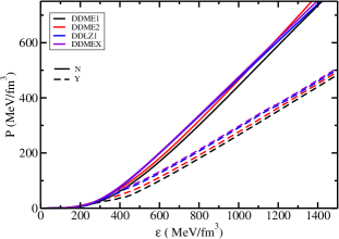
The EoS of pure nucleonic (solid lines) and hyperonic matter (dashed lines) under chemical-equilibrium and charge neutrality conditions for several DD-RMF parameter sets are displayed in figure 1. For pure nucleonic matter, the DD-MEX parameter set produces a stiff EoS at low density region, while the DD-ME2 set produces a stiff EoS in the high density regime. The hyperons start to appear in the density range 300-400 MeV/fm3 for all parameter sets. The onset of hyperonization softens the EoS (reduction in the pressure) due to the hyperons replacing the neutrons and opening new channels to distribute the Fermi energy. To build a unified EoS, the Baym-Pethick-Sutherland (BPS) EoS (Baym et al., 1971) has been used in the outer crust region. For the inner crust part, the EoS for non-uniform matter is generated by using DD-ME2 parameter set in a Thomas-Fermi approximation (Avancini et al., 2009; Pais & Providência, 2016; Rather et al., 2021b). All the DD-RMF parameter sets considered are very similar in the outer crust density regime.
With the EoSs obtained for pure nucleonic and hyperonic matter, stellar matter properties like mass and radius are obtained by solving the Tolmann-Oppenheimer-Volkov (TOV) coupled differential equations (Tolman, 1939; Oppenheimer & Volkoff, 1939) for a static isotropic spherically symmetric star
| (21) |
and
| (22) |
where contained in the radius represents the gravitational mass for a specific EoS and a given choice of central energy density .
The tidal deformability is defined as (Hinderer et al., 2010; Kumar et al., 2017)
| (23) |
where, represents the mass quadrupole moment of a star and corresponds to its external tidal field. The dimensionless tidal deformability is related to the compactness parameter as
| (24) |
where is the second love number. To estimate the love number along with the evaluation of the TOV equations, the function as defined in ref (Hinderer, 2008) is computed with the initial condition of for the second love number. This value can be computed from the following first-order differential equations (Kumar et al., 2017; Hinderer, 2008)
| (25) |
where,
| (26) | ||||
| (27) |
Once the above equations are solved for with being the radius of the spherical star in isolation, the second tidal love number is obtained from the following expression (Hinderer et al., 2010)
| (28) |
Given the initial boundary conditions for the NS at the center , , and with as the central pressure, to the surface of the star , , and , the above equations are solved for a given central density to determine the macroscopic properties of a NS.
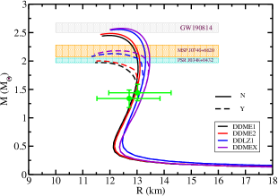
Figure 2 shows the mass-radius relation for pure nucleonic and hyperonic matter for the parameter sets DD-ME1, DD-ME2, DD-LZ1, and DD-MEX. The shaded areas represent the recent constraints on the NS maximum mass inferred from GW190814 (M=2.50-2.67 ), the massive pulsars MSP J0740+6620 (M=2.14 ), and PSR J0348+0432 (M=2.01 ). The constraints on the radius limits around the NS canonical mass inferred from PSR J0030+0451 by NICER, R=13.02 km at M=1.44 (Miller et al., 2019) and R=12.71 km at M=1.34 (Riley et al., 2019), are also shown. For pure nucleonic matter, the DD-LZ1 and DD-MEX parameter sets reach a maximum mass of 2.55 and 2.57 , with a radius of 12.30 and 12.46 km, respectively, indicating the possibility of GW190814 secondary component being a very massive NS. The hyperonic counterparts of the given DD-RMF parameter sets, which soften the EoS, produce a maximum mass of 2.18 and 2.13 with a radius of 12.24 and 12.07 km respectively. For the DD-ME1 and DD-ME2 parameter sets, the NS maximum mass decreases from 2.45 and 2.48 to 1.98 and 2.01 respectively, while the respective radius decreases by 0.5 km. The radius at the NS canonical mass, R1.4, remains insensitive to the appearance of hyperons. The hyperonic configurations satisfy the maximum mass limit from the massive pulsars MSP J0740+6620 and PSR J0348+0432, but are inconsistent with the GW190814 potential constraint (see discussion in Sedrakian et al. (2020a)). All of the nucleonic and hyperonic configurations satisfy the mass-radius limits inferred from NICER.
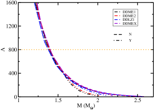
The variation of the dimensionless tidal deformability with the NS mass for the nucleonic and hyperonic stars based on the DD-RMF parametrizations are shown in figure 3. The dimensionless tidal deformability of pure nucleonic as well as hyperonic matter for all the parameter sets lies well below the upper limit of =800 obtained from the gravitational wave event GW170817 (Abbott et al., 2017). The shift in the tidal deformability for the hyperonic matter is seen as the mass increases. Table 2 displays the different properties of neutron and hyperonic stars obtained with different DD-RMF parameter sets. A subsequent analysis by the LVC suggest a much smaller upper limit of 580 on the tidal deformability, which is smaller than all the values displayed in Table 2 Abbott et al. (2018). However, this value corresponds to the 50% confidence region, the 90% confidence region extracted from the same data includes the values we reproduce.
m respective radius, and radius and dimensionless tidal deformability of a 1.4 star.
9.7cm Nucleonic star Hyperonic star Mmax () R (km) R1.4 (km) Mmax () R (km) R1.4 (km) DD-ME1 2.449 11.981 12.898 689.342 1.983 11.515 12.898 689.342 DD-ME2 2.483 12.017 12.973 733.149 2.013 11.674 12.973 733.149 DD-LZ1 2.555 12.297 13.069 728.351 2.130 12.067 13.069 728.351 DD-MEX 2.575 12.465 13.168 791.483 2.183 12.238 13.168 791.483
4.2 Magnetic stars
In order to study the effects of magnetic fields on our microscopic description of matter, we employ a chemical potential-dependent magnetic field derived from the solutions of the Einstein-Maxwell’s equations. The quadratic relation between the magnetic field and the chemical potential depends on the magnetic dipole moment and is given by (Dexheimer et al., 2017a)
| (29) |
with being the baryon chemical potential in MeV and the dipole magnetic moment in units of Am2 to produce in units of the electron critical field G. The coefficients , , and taken as G2/(Am2), G2/(Am2 MeV) and G2/(Am2 MeV2) are obtained from a fit for the magnetic field in the polar direction of a star with a baryon mass of 2.2 .
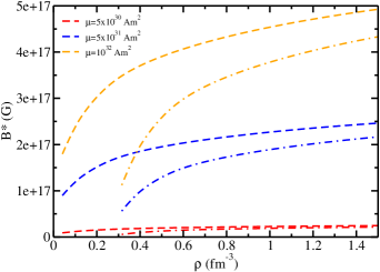
Figure 4 displays the magnetic field profile as a function of baryon density for a 2.2 baryonic mass star obtained for the DD-MEX EoS. The magnetic field effect on the DD-ME2 EoS has already been calculated (Thapa et al., 2020) and the DD-ME1 EoS predicts similar behavior. In Ref. (Thapa et al., 2020), spherically symmetric TOV equations were used for central magnetic fields 1018 G with a density-dependent and universal profile for magnetic field. Since the DD-MEX EoS predicts a heavier NS than other parameter sets, we choose this parameter set to study magnetic effects and verify whether this model predicts the possibility of the GW190814 secondary component being a hyperonic magnetar. In fig. 4, the dashed curves represent a NS without hyperons and dot-dashed curves represent a NS with hyperons. It is clear that the magnetic field produced by the NS without hyperons is larger. This illustrates that the transition from to is model and particle population dependent. For magnetic dipole moment greater than 1031 Am2, the magnetic field produced at large densities is larger than 1017 G, which is strong enough to cause a large deformation in the NS structure. The values of the magnetic field produced at the surface and at large densities using different values of the magnetic dipole moment for NSs with and without hyperons are shown in table 3. For a magnetic dipole moment 1032 Am2, the magnetic field produced at large densities is greater than 4 1017 for both cases.
| Nucleonic star | Hyperonic star | |||
|---|---|---|---|---|
| (Am2) | Bs (G) | Bc (G) | Bs (G) | Bc (G) |
| 51030 | 1.011015 | 2.591016 | 6.651015 | 1.961016 |
| 51031 | 8.981016 | 2.281017 | 5.831016 | 1.891017 |
| 1032 | 1.791017 | 4.551017 | 1.121017 | 3.771017 |
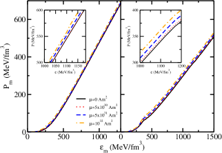
Figure 5 shows the variation of the transverse pressure vs the energy density for the DD-MEX parameter set with and without hyperons. The solid line represents the variation in the pressure without including magnetic field (=0), while the other lines represent the variation obtained with the magnetic field at magnetic dipole moments =51030 Am2, 51031 Am2 and 1030 Am2. The insets show the pressure at higher values of the energy density. It is clear that the change in the pressure at a given value of energy density is larger for a NS with hyperons as compared to the NS without hyperons, which implies that the EoS with hyperons becomes stiffer than without hyperons (when compared to the = 0 case) in the presence of strong magnetic field. The reason for such behavior will be discussed in the following. The magnetic field produced at the magnetic dipole moment 51030 Am2 is of the order of 1016 G at the center, which is small enough to be indistinguishable from the zero magnetic case. For higher magnetic dipole moments, the magnetic field produced 4 1017 G is strong enough to increase the matter pressure to higher values, thus producing a distinguishable effect.
Figure 6 shows the particle fractions as a function of baryon density for beta stable NS matter obtained using the DD-MEX EoS. Figure 6 panel (a) displays the fractions in the absence of magnetic field, while panels (b), (c), and (d) depict the particle fractions in the presence of magnetic fields with fixed magnetic dipole moments =51030 Am2, =51031 Am2, and =51032 Am2, respectively. Clearly, in all the cases, the particle is the dominant hyperonic component, which starts appearing in the density range 2 - 3 (DHapo et al., 2010; Vidaña, 2013; Rather et al., 2018; Sen et al., 2018). The neutral hyperon appears at a density 5.5 for =0, which remains unaltered with the inclusion of the magnetic field. As expected, the charged particles are more strongly affected by the magnetic field and an increase in their population is seen with the increase in the magnetic field strength. For =0 (and all other cases), the and population is large at low densities, which suppresses the appearance of hyperons. With an increase in the magnetic dipole moment, the magnetic field strength increases, which shifts the appearance of hyperon from 2.5 to around 3.5. At this threshold, the density of the negatively charged leptons and starts to drop, as the charge neutrality condition from (2) allows the hyperon to take over. Similarly, the appearance of the hyperon accelerates the disappearance of neutrons, as both are neutral particles. Overall, we see that the addition of magnetic field increases the population of leptons (re-leptonizes) and correspondingly decreases the population of hyperons (de-hyperonizes), which renders the EoS stiffer (Tolos et al., 2016).
Because of the repulsive nature of the potential, the formation of and is totally suppressed for the densities considered in the present work. The absence of hyperons is supported by the fact that no bound hypernuclei has been found yet, despite several searches (Harada & Hirabayashi, 2006, 2015) and this has been reproduced in several works (Glendenning, 2001; Thapa et al., 2020; Guichon et al., 2018). The inclusion of strong magnetic fields do not change this feature. The properties of nucleonic and hyperonic stars at different values of the magnetic dipole moment, which correspond to different magnetic field values at the surface and the center, are shown in table 4.
The effect of magnetic field on the mass-radius relation of a NS with and without hyperons is displayed in figure 7. These calculations are performed for the DD-MEX EoS using the LORENE library (LORENE, -). Different values of magnetic dipole moment are used to obtain different values of the magnetic field at the stellar surface and at the center. As can be seen, the NS maximum mass without hyperons increases from 2.575 for =0 to 2.711 for =1032 Am2. The corresponding radius changes from 12.465 to 13.474 km. The radius at 1.4 increases by around 1 km. With the hyperons included, the mass increases from 2.183 to 2.463 when magnetic field effects are included with =1032 Am2. The variation obtained in the mass-radius is larger for hyperonic stars than for the pure nucleonic stars due to the additional effect of de-hyperonization that takes place due to the magnetic field. The de-hyperonization results in the enhancement of the matter pressure for a given .
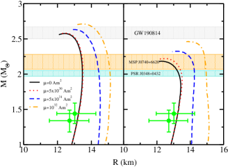
For higher magnetic fields produced at magnetic dipole moments =5 1031 and =1032 Am2, the effect of the magnetic field is seen to be very large at smaller stellar masses. For low magnetic fields, pure nucleonic stars still satisfy the possible maximum mass constraint from the GW190814 event, implying the possibility that of its secondary component to be a magnetar. The radius constraints inferred from NICER are satisfied by both nucleonic as well as hyperonic stars with low magnetic fields. For central magnetic fields 7 1016 G, the EoS obtained for pure nucleonic matter satisfies the radius constraints from NICER measurement. For hyperonic matter, a lower magnetic field 4 1016 G produces a hyperonic star with radius that satisfies NICER constraints. This is due to the fact that for magnetic fields less than 1017 G, the deformation produced in the stellar structure is negligible and, hence, the variation in radius is too small when compared to the non-magnetic case. Note that the surface magnetic field of the stars observed by NICER is expected to be G (Miller et al., 2019).
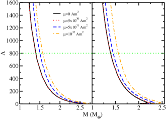
Figure 8 shows the variation in the dimensionless tidal deformability as a function of gravitational mass with magnetic field effects and considering different values of magnetic dipole moment. The results for EoS with and without hyperons are shown. For pure nucleonic stars, the tidal deformability increases to a value 1500 for a central magnetic field of 4.55 1017 G produced fixing the magnetic dipole moment to =1032 Am2, thus violating the constraint on the dimensionless tidal deformability from GW170817, which provides an upper limit of 800 on at 90% confidence (Abbott et al., 2017). Seen in table 4, a small magnetic field produces a NS with tidal deformability larger than the upper limit from GW170817. This confirms that the BNS merger event GW170817 did not consist of magnetars.
m dimensionless tidal deformability () of pure nucleonic and hyperonic star for the DD-MEX EoS without magnetic field
m and with magnetic field effects for different values of the magnetic dipole moment.
9.5cm (Am2) Nucleonic star Hyperonic star Mmax () R (km) R1.4 (km) Mmax () R (km) R1.4 (km) 0 2.575 12.465 13.168 791.483 2.183 12.238 13.168 791.483 5 1030 2.580 12.536 13.235 802.801 2.224 12.506 13.168 791.483 5 1031 2.632 13.024 14.507 1175.35 2.325 13.269 14.112 998.882 1032 2.711 13.474 15.027 1517.09 2.463 13.894 15.105 1559.194
For hyperonic stars, the value at 1.4 remains unchanged when considering a magnetic dipole moment of =5 1030 Am2. As the magnetic dipole moment increases, stronger magnetic fields increase the stellar radius, which allows the tidal deformability to reach a value around 1550. For a nucleonic star and a hyperonic star with dimensionless tidal deformability well within the limit of GW170817 at 90% confidence, a magnetic field with a maximum value of 2 1016 G is required. See Ref (Biswas & Bose, 2019) for a discussion of the tidal deformability of deformed stars and Ref. (Zhu et al., 2020) for a discussion on how very large magnetic fields generate new high-order corrections to the deformability that can modify the gravitational-wave evolution of magnetars. Note that magnetic NSs can also be a source of gravitational waves due to their asymmetric nature (Sur & Haskell, 2021; Haskell et al., 2008; Gomes et al., 2019; Bonazzola & Gourgoulhon, 1996; Frieben & Rezzolla, 2012).
4.3 Additional hyperon couplings
To investigate how different hyperon couplings and hyperon potentials affect the results we presented so far, we use a more general symmetry group SU(3) to determine the coupling constants of all baryons and mesons (Lopes & Menezes, 2014, 2021). For the meson, we have
| (30) |
For the meson, we have
| (31) |
The hyperon-scalar meson coupling constants are fixed so as to reproduce the following optical potentials (Glendenning & Moszkowski, 1991; Dover & Gal, 1984; Schaffner et al., 1994; Schaffner-Bielich & Gal, 2000)
| (32) |
The coupling constants at different values of the parameter are displayed in table 5. For = 1.0, the hybrid SU(6) group is recovered.
| = 1.0 | = 0.75 | = 0.50 | = 0.25 | |
|---|---|---|---|---|
| 0.667 | 0.687 | 0.714 | 0.75 | |
| 0.667 | 0.812 | 1.00 | 1.25 | |
| 0.333 | 0.437 | 0.571 | 0.75 | |
| 2.0 | 1.5 | 1.0 | 0.5 | |
| 1.0 | 0.5 | 0.0 | -0.5 | |
| 0.610 | 0.626 | 0.653 | 0.729 | |
| 0.403 | 0.514 | 0.658 | 0.850 | |
| 0.318 | 0.398 | 0.500 | 0.638 |
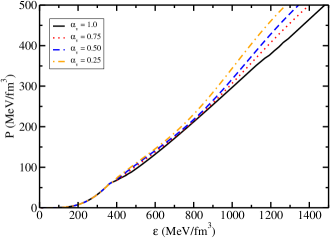
The particle population of hyperons and other particles depend upon the hyperon meson coupling constants, which vary with the parameter . Changing the value of from 1.0 to 0.25 suppresses strange particles. The suppression of increases the lepton fraction at lower value of . The neutrons and protons are the most populated particles at =0.25. Figure 9 displays the EoS obtained using different values of the parameter . As the value decreases from 1.0 to 0.25, the stiffness of the EoS increases due to the increase in the value of meson couplings.
Figure 10 displays the mass-radius relation for hyperonic stars without magnetic field effects at different values of . Lowering the value of stiffens the EoS, which increases the maximum mass to 2.283 for =0.25 (from 2.183 for =1.0). It is to be mentioned that the stellar properties of hyperonic stars obtained at =1.0 almost resemble to that obtained from the hyperon potentials given by (3). The change in the hyperon potentials alters the values of sigma meson couplings by a small fraction and, hence, the changes obtained in the particle population and stellar properties are negligible.
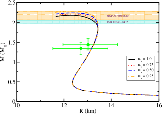
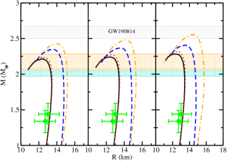
With the addition of magnetic field effects, the results of different hyperon couplings on hyperonic EoSs is determined. Figure 11 displays the relation between mass and radius for a hyperonic star at different values without magnetic field and with magnetic field effects considered at different values of magnetic dipole moment. For =0.75, the maximum mass increases to a value 2.437 for a magnetic dipole moment =1032 Am2, which corresponds to a central magnetic field of 3.77 1017 G. Similarly, for =0.50 and 0.25, the maximum mass reaches a value 2.480 and 2.556, respectively, at =1032 Am2. This implies that the secondary component of GW190814 could be a hyperonic magnetar. For the present, hyperon couplings with a magnetic dipole moment =5 1031 Am2, which corresponds to a central magnetic field greater than 1017 G, the deviation in the hyperonic star radius at canonical mass is very large, around 1.5 km, as compared to that obtained from previous couplings. But with even stronger magnetic fields, the deviation obtained is less in the present case. This implies that a change in hyperon couplings effects the stellar properties, especially the radius at canonical mass at strong central magnetic field.
9.7cm (Am2) =0.75 =0.50 =0.25 Mmax () R (km) R1.4 (km) Mmax () R (km) R1.4 (km) Mmax () R (km) R1.4 (km) 0 2.217 12.335 13.168 791.483 2.239 12.335 13.168 791.483 2.283 12.453 13.168 791.483 5 1030 2.240 12.543 13.213 815.398 2.271 12.632 13.224 869.281 2.316 12.652 13.237 914.012 5 1031 2.349 13.522 14.741 1338.714 2.366 13.708 14.821 1397.389 2.407 13.563 14.938 1425.185 1032 2.437 13.995 14.992 1510.783 2.480 14.224 15.069 1615.288 2.556 14.469 15.403 1879.880
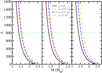
Figure 12 displays the variation in the dimensionless tidal deformability of a hyperonic star with magnetic field effects considered at different values of magnetic dipole moment. For small values of the magnetic dipole moment at different values of , the -M curve follows similar pattern as for the previous hyperon couplings. Since the variation in radius at canonical mass are large for the present couplings, the tidal deformability, obtained is also large. For =0.25, the dimensionless tidal deformability reaches a value of 1900 for magnetic dipole moment 1032 Am2. The properties of hyperonic stars using different hyperon coupling values according to the value of with and without magnetic field effects considered at different magnetic dipole moments, are shown in table 6.
5 Summary and Conclusion
We modeled massive nucleonic and hyperonic stars that fulfill the constraints set by the observation of the possibly most massive neutron star (NS) ever detected (in the secondary object of the gravitational wave event GW190814) using a density-dependent relativistic mean field model (DD-RMF). This simple, yet powerful formalism provides the freedom necessary to fulfill simultaneously nuclear and astrophysical constraints. The results obtained from the TOV equations show that the hyperons soften the EoS, lowering the maximum mass of NS to around 2.2, thereby satisfying more conservative massive constraints from the astrophysical observations. The radius of the NS canonical mass is seen to be insensitive to the appearance of hyperons. Both the nucleonic and the hyperonic stars satisfy the constraints from mass-radius limits inferred from NICER observations and tidal deformability constraints from the LIGO and VIRGO collaborations.
We also studied the effects of strong magnetic fields on DD-RMF nucleonic and hyperonic EoSs. We investigated the EoS and particle populations using a realistic chemical potential-dependent magnetic field that was developed by solving Einstein-Maxwell equations. For very strong magnetic fields, the spherical symmetric solutions obtained by solving the TOV equations lead to an overestimation of the mass and the radius and, hence, cannot be used for determining stellar properties. For this reason, we used the LORENE library to determine stellar properties of magnetic NSs. For low values of the magnetic dipole moment, implying lower strengths of magnetic fields, the EoS resembles the non-magnetic one. For higher magnetic dipole moments, the EoS stiffens at higher energy density. The amount of stiffness is larger in case of hyperonic EoSs than for the case of pure nucleonic ones. As the magnetic field strength is increased, the particle fractions of leptons ( and ) increases at higher densities and the appearance of charged hyperons () is delayed.
The stiffening in the EoS caused by the changes in population described above increases the maximum mass of magnetic stars. For a small dipole moment of 5 1030 Am2, the nucleonic and hyperonic mass-radius profiles resemble the non-magnetic case due to the lower magnetic field produced. For higher magnetic dipole moments, although the variation in the maximum mass is small, a variation of about 1 km is seen in the radius of the NS canonical mass. For hyperonic stars, the maximum mass increases by 0.3 , allowing them to satisfy the GW190814 possible mass constraint for a dipole moment Am2 when different coupling schemes are considered. For strong magnetic fields, the different coupling schemes for hyperons predict increases in radius of km. Thus, we see that different hyperon couplings and different hyperon potentials populate stellar matter differently and, hence, can change stellar properties significantly.
The change in the dimensionless tidal deformability for NS was studied. It was found that, for higher value of the magnetic dipole moment, the tidal deformability of the canonical mass surpasses the upper limit of 800 set by the measurement from GW1701817 at 90% confidence, which is consistent with the acknowledgement of such objects possessing weak magnetic fields. No such measurement of tidal deformability is available for GW190814, as it has no tidal signatures. But if in the future, measurements of tidal deformability of massive NSs such as the one measured for the secondary object in GW190814 are 800, this would imply that object could not be a hyperonic magnetar.
In the future, we will investigate the effect of considering more exotic particles in our modelling of magnetic NSs. These include, kaons, -resonances and deconfined quark matter (with and without mixtures of phases). We also intend to analyze combined effects of magnetic fields and fast rotation on stars containing exotic matter, as both of these aspects could be important in young stars (Lasky et al., 2019; Yu et al., 2019; Lasky et al., 2017).
Appendix A
Within the relativistic density-dependent mean field (DD-RMF) model, the equation of motion for baryons obtained by applying the Euler Lagrange equations to the Lagrangian density (2) is written as
| (A.1) |
where, is the effective mass of baryons and is the rearrangment term due to the density dependence of the coupling constants
| (A.2) |
The equation of motion for meson fields are
| (A.3) |
where the scalar density , baryon density , and isovector densities , and , are given as
| (A.4) |
With the above equations, the expression for the energy density and pressure are
| (A.5) |
where, . The rearrangment term contributes to the pressure only.
In the presence of magnetic field, the scalar and vector density for charged baryons , uncharged baryons , and leptons follow as (Broderick et al., 2000)
| (A.6) |
where is the Landau degeneracy of level. The expressions for the baryon and lepton energy densities in the presence of magnetic field become
| (A.7) |
References
- Abbott et al. (2017) Abbott, B. P., Abbott, R., et al. 2017, Phys. Rev. Lett., 119, 161101, doi: 10.1103/PhysRevLett.119.161101
- Abbott et al. (2018) —. 2018, Phys. Rev. Lett., 121, 161101, doi: 10.1103/PhysRevLett.121.161101
- Abbott et al. (2019) —. 2019, Phys. Rev. X, 9, 011001, doi: 10.1103/PhysRevX.9.011001
- Abbott et al. (2020a) Abbott, R., Abbott, T. D., et al. 2020a, Astrophys. Jour., 896, L44, doi: 10.3847/2041-8213/ab960f
- Abbott et al. (2020b) Abbott, R., et al. 2020b, Astrophys. J. Lett., 896, L44, doi: 10.3847/2041-8213/ab960f
- Adhikari et al. (2021) Adhikari, D., Albataineh, H., Androic, D., et al. 2021, Phys. Rev. Lett., 126, 172502, doi: 10.1103/PhysRevLett.126.172502
- Aguirre (2019) Aguirre, R. M. 2019, Phys. Rev. C, 100, 065203, doi: 10.1103/PhysRevC.100.065203
- Aguirre (2020) —. 2020, Phys. Rev. D, 102, 096025, doi: 10.1103/PhysRevD.102.096025
- Ambartsumyan & Saakyan (1960) Ambartsumyan, V. A., & Saakyan, G. S. 1960, Sov. Astron., 4, 187. https://ui.adsabs.harvard.edu/abs/1960SvA.....4..187A
- Antoniadis & Freire et al. (2013) Antoniadis, J., & Freire et al., P. C. C. 2013, Science, 340, doi: 10.1126/science.1233232
- Avancini et al. (2009) Avancini, S. S., Brito, L., Marinelli, J. R., et al. 2009, Phys. Rev. C, 79, 035804, doi: 10.1103/PhysRevC.79.035804
- Avancini et al. (2018) Avancini, S. S., Dexheimer, V., Farias, R. L. S., & Timóteo, V. S. 2018, Phys. Rev. C, 97, 035207, doi: 10.1103/PhysRevC.97.035207
- Baldo et al. (2000) Baldo, M., Burgio, G. F., & Schulze, H. J. 2000, Phys. Rev. C, 61, 055801, doi: 10.1103/PhysRevC.61.055801
- Bandyopadhyay et al. (1997) Bandyopadhyay, D., Chakrabarty, S., & Pal, S. 1997, Phys. Rev. Lett., 79, 2176, doi: 10.1103/PhysRevLett.79.2176
- Banik & Bandyopadhyay (2001) Banik, S., & Bandyopadhyay, D. 2001, Phys. Rev. C, 64, 055805, doi: 10.1103/PhysRevC.64.055805
- Banik et al. (2014) Banik, S., Hempel, M., & Bandyopadhyay, D. 2014, Astrophys. Jour. Suppl. Ser., 214, 22, doi: 10.1088/0067-0049/214/2/22
- Baym et al. (1971) Baym, G., Pethick, C., & Sutherland, P. 1971, Astrophys. J., 170, 299, doi: 10.1086/151216
- Beloborodov (2020) Beloborodov, A. M. 2020, Astrophys. Jour., 896, 142, doi: 10.3847/1538-4357/ab83eb
- Beniamini et al. (2020) Beniamini, P., Wadiasingh, Z., & Metzger, B. D. 2020, MNRAS, 496, 3390, doi: 10.1093/mnras/staa1783
- Bhowmick et al. (2014) Bhowmick, B., Bhattacharya, M., Bhattacharyya, A., & Gangopadhyay, G. 2014, Phys. Rev. C, 89, 065806, doi: 10.1103/PhysRevC.89.065806
- Biswas & Bose (2019) Biswas, B., & Bose, S. 2019, Phys. Rev. D, 99, 104002, doi: 10.1103/PhysRevD.99.104002
- Biswas et al. (2020) Biswas, B., Nandi, R., Char, P., Bose, S., & Stergioulas, N. 2020, GW190814: On the properties of the secondary component of the binary. https://arxiv.org/abs/2010.02090
- Bocquet et al. (1995) Bocquet, M., Bonazzola, S., Gourgoulhon, E., & Novak, J. 1995, Astron. Astrophys., 301, 757. https://ui.adsabs.harvard.edu/abs/1995A&A...301..757B
- Bombaci et al. (2020) Bombaci, I., Drago, A., Logoteta, D., Pagliara, G., & Vidaña, I. 2020, Was GW190814 a black hole – strange quark star system? https://arxiv.org/abs/2010.01509
- Bombaci et al. (2021) —. 2021, Phys. Rev. Lett., 126, 162702, doi: 10.1103/PhysRevLett.126.162702
- Bonazzola & Gourgoulhon (1996) Bonazzola, S., & Gourgoulhon, E. 1996, Astron. Astrophys., 312, 675. https://arxiv.org/abs/astro-ph/9602107
- Bonazzola et al. (1993) Bonazzola, S., Gourgoulhon, E., Salgado, M., & Marck, J. A. 1993, Astron. Astrophys., 278, 421. https://ui.adsabs.harvard.edu/abs/1993A&A...278..421B
- Bransgrove et al. (2017) Bransgrove, A., Levin, Y., & Beloborodov, A. 2017, MNRAS, 473, 2771, doi: 10.1093/mnras/stx2508
- Brockmann & Toki (1992) Brockmann, R., & Toki, H. 1992, Phys. Rev. Lett., 68, 3408, doi: 10.1103/PhysRevLett.68.3408
- Broderick et al. (2000) Broderick, A., Prakash, M., & Lattimer, J. M. 2000, Astrophys. Jour., 537, 351, doi: 10.1086/309010
- Cao et al. (2020) Cao, Z., Chen, L.-W., Chu, P.-C., & Zhou, Y. 2020, GW190814: Circumstantial Evidence for Up-Down Quark Star. https://arxiv.org/abs/2009.00942
- Cardall et al. (2001) Cardall, C. Y., Prakash, M., & Lattimer, J. M. 2001, Astrophys. Jour., 554, 322, doi: 10.1086/321370
- Casali et al. (2014) Casali, R. H., Castro, L. B., & Menezes, D. P. 2014, Phys. Rev. C, 89, 015805, doi: 10.1103/PhysRevC.89.015805
- Chakrabarty et al. (1997) Chakrabarty, S., Bandyopadhyay, D., & Pal, S. 1997, Phys. Rev. Lett., 78, 2898, doi: 10.1103/PhysRevLett.78.2898
- Chatterjee et al. (2015) Chatterjee, D., Elghozi, T., Novak, J., & Oertel, M. 2015, MNRAS, 447, 3785, doi: 10.1093/mnras/stu2706
- Chatterjee & Vidaña (2016) Chatterjee, D., & Vidaña, I. 2016, Eur. Phys. J. A, 52, 29, doi: 10.1140/epja/i2016-16029-x
- Chatterjee & Vidaña (2016) Chatterjee, D., & Vidaña, I. 2016, Eur. Phys. Jour. A, 52, 29, doi: 10.1140/epja/i2016-16029-x
- Chen & Piekarewicz (2015) Chen, W.-C., & Piekarewicz, J. 2015, Phys. Rev. Lett., 115, 161101, doi: 10.1103/PhysRevLett.115.161101
- Christian & Schaffner-Bielich (2021a) Christian, J.-E., & Schaffner-Bielich, J. 2021a, Phys. Rev. D, 103, 063042, doi: 10.1103/PhysRevD.103.063042
- Christian & Schaffner-Bielich (2021b) —. 2021b, Phys. Rev. D, 103, 063042, doi: 10.1103/PhysRevD.103.063042
- Ciolfi et al. (2019) Ciolfi, R., Kastaun, W., Kalinani, J. V., & Giacomazzo, B. 2019, Phys. Rev. D, 100, 023005, doi: 10.1103/PhysRevD.100.023005
- Colucci & Sedrakian (2014) Colucci, G., & Sedrakian, A. 2014, J. Phys. Conf. Ser., 496, 012003, doi: 10.1088/1742-6596/496/1/012003
- Cromartie & Fonseca et al. (2019) Cromartie, H. T., & Fonseca et al., E. 2019, Nature Astron., 4, 72, doi: 10.1038/s41550-019-0880-2
- Dall’Osso et al. (2018) Dall’Osso, S., Stella, L., & Palomba, C. 2018, Mon. Not. Roy. Astron. Soc., 480, 1353, doi: 10.1093/mnras/sty1706
- Danielewicz & Lee (2014) Danielewicz, P., & Lee, J. 2014, Nucl. Phys. A, 922, 1 , doi: https://doi.org/10.1016/j.nuclphysa.2013.11.005
- Demircik et al. (2021a) Demircik, T., Ecker, C., & Järvinen, M. 2021a, Astrophys. J. Lett., 907, L37, doi: 10.3847/2041-8213/abd853
- Demircik et al. (2021b) Demircik, T., Ecker, C., & Järvinen, M. 2021b, The Astrophys. Jour., 907, L37, doi: 10.3847/2041-8213/abd853
- Demorest et al. (2010) Demorest, P. B., Pennucci, T., Ransom, S. M., Roberts, M. S. E., & Hessels, J. W. T. 2010, Nature, 467, 1081, doi: 10.1038/nature09466
- Dexheimer et al. (2017a) Dexheimer, V., Franzon, B., Gomes, R., et al. 2017a, Phys. Lett. B, 773, 487, doi: https://doi.org/10.1016/j.physletb.2017.09.008
- Dexheimer et al. (2017b) Dexheimer, V., Franzon, B., Gomes, R. O., et al. 2017b, Phys. Lett. B, 773, 487, doi: 10.1016/j.physletb.2017.09.008
- Dexheimer et al. (2021) Dexheimer, V., Gomes, R. O., Klähn, T., Han, S., & Salinas, M. 2021, Phys. Rev. C, 103, 025808, doi: 10.1103/PhysRevC.103.025808
- Dexheimer et al. (2012) Dexheimer, V., Negreiros, R., & Schramm, S. 2012, Eur. Phys. J. A, 48, 189, doi: 10.1140/epja/i2012-12189-y
- Dexheimer & Schramm (2008) Dexheimer, V., & Schramm, S. 2008, Astrophys. J., 683, 943, doi: 10.1086/589735
- DHapo et al. (2010) DHapo, H., Schaefer, B.-J., & Wambach, J. 2010, Phys. Rev. C, 81, 035803, doi: 10.1103/PhysRevC.81.035803
- Dhiman et al. (2007) Dhiman, S. K., Kumar, R., & Agrawal, B. K. 2007, Phys. Rev. C, 76, 045801, doi: 10.1103/PhysRevC.76.045801
- Dover & Gal (1984) Dover, C., & Gal, A. 1984, Prog. Part. and Nucl. Phys., 12, 171, doi: https://doi.org/10.1016/0146-6410(84)90004-8
- Fattoyev et al. (2020) Fattoyev, F. J., Horowitz, C. J., Piekarewicz, J., & Reed, B. 2020, Phys. Rev. C, 102, 065805, doi: 10.1103/PhysRevC.102.065805
- Fattoyev et al. (2018) Fattoyev, F. J., Piekarewicz, J., & Horowitz, C. J. 2018, Phys. Rev. Lett., 120, 172702, doi: 10.1103/PhysRevLett.120.172702
- Felipe et al. (2008) Felipe, R. G., Martinez, A. P., Rojas, H. P., & Orsaria, M. 2008, Phys. Rev. C, 77, 015807, doi: 10.1103/PhysRevC.77.015807
- Fortin et al. (2017) Fortin, M., Avancini, S. S., Providência, C., & Vidaña, I. 2017, Phys. Rev. C, 95, 065803, doi: 10.1103/PhysRevC.95.065803
- Fortin et al. (2020) Fortin, M., Raduta, A. R., Avancini, S., & Providência, C. 2020, Phys. Rev. D, 101, 034017, doi: 10.1103/PhysRevD.101.034017
- Fortin et al. (2021) Fortin, M., Raduta, A. R., Avancini, S., & Providencia, C. 2021, Phys. Rev. D, 103, 083004, doi: 10.1103/PhysRevD.103.083004
- Frieben & Rezzolla (2012) Frieben, J., & Rezzolla, L. 2012, Mon. Not. Roy. Astron. Soc., 427, 3406, doi: 10.1111/j.1365-2966.2012.22027.x
- Gendreau et al. (2016) Gendreau, K. C., Arzoumanian, Z., et al. 2016, in Society of Photo-Optical Instrumentation Engineers (SPIE) Conference Series, Vol. 9905, Space Telescopes and Instrumentation 2016: Ultraviolet to Gamma Ray, ed. J.-W. A. den Herder, T. Takahashi, & M. Bautz, 99051H, doi: 10.1117/12.2231304
- Giacomazzo et al. (2015) Giacomazzo, B., Zrake, J., Duffell, P., MacFadyen, A. I., & Perna, R. 2015, Astrophys. J., 809, 39, doi: 10.1088/0004-637X/809/1/39
- Glendenning (1982) Glendenning, N. K. 1982, Phys. Lett. B, 114, 392, doi: https://doi.org/10.1016/0370-2693(82)90078-8
- Glendenning (1985) Glendenning, N. K. 1985, Astrophys. Jour., 293, 470, doi: 10.1086/163253
- Glendenning (2001) Glendenning, N. K. 2001, Phys. Rev. C, 64, 025801, doi: 10.1103/PhysRevC.64.025801
- Glendenning & Moszkowski (1991) Glendenning, N. K., & Moszkowski, S. A. 1991, Phys. Rev. Lett., 67, 2414, doi: 10.1103/PhysRevLett.67.2414
- Godzieba et al. (2021) Godzieba, D. A., Radice, D., & Bernuzzi, S. 2021, Astrophys. J., 908, 122, doi: 10.3847/1538-4357/abd4dd
- Gomes et al. (2015) Gomes, R. O., Dexheimer, V., Schramm, S., & Vasconcellos, C. A. Z. 2015, Astrophys. J., 808, 8, doi: 10.1088/0004-637X/808/1/8
- Gomes et al. (2017) Gomes, R. O., Franzon, B., Dexheimer, V., & Schramm, S. 2017, Astrophys. J., 850, 20, doi: 10.3847/1538-4357/aa8b68
- Gomes et al. (2019) Gomes, R. O., Pais, H., Dexheimer, V., Providência, C., & Schramm, S. 2019, Astron. Astrophys., 627, A61, doi: 10.1051/0004-6361/201935310
- Goncalves & Lazzari (2020) Goncalves, V. P., & Lazzari, L. 2020, Phys. Rev. D, 102, 034031, doi: 10.1103/PhysRevD.102.034031
- Gonçalves & Lazzari (2020) Gonçalves, V. P., & Lazzari, L. 2020, Phys. Rev. D, 102, 034031, doi: 10.1103/PhysRevD.102.034031
- Guichon et al. (2018) Guichon, P. A. M., Stone, J. R., & Thomas, A. W. 2018, Prog. Part. Nucl. Phys., 100, 262, doi: 10.1016/j.ppnp.2018.01.008
- Gupta et al. (2020) Gupta, A., Gerosa, D., Arun, K. G., et al. 2020, Phys. Rev. D, 101, 103036, doi: 10.1103/PhysRevD.101.103036
- Gusakov et al. (2014) Gusakov, M. E., Haensel, P., & Kantor, E. M. 2014, Mon. Not. Roy. Astron. Soc., 439, 318, doi: 10.1093/mnras/stt2438
- Harada & Hirabayashi (2006) Harada, T., & Hirabayashi, Y. 2006, Nucl. Phys. A, 767, 206, doi: https://doi.org/10.1016/j.nuclphysa.2005.12.018
- Harada & Hirabayashi (2015) —. 2015, Phys. Lett. B, 740, 312, doi: https://doi.org/10.1016/j.physletb.2014.11.057
- Harding & Lai (2006) Harding, A. K., & Lai, D. 2006, Rep. Prog. Phys., 69, 2631, doi: 10.1088/0034-4885/69/9/r03
- Haskell et al. (2008) Haskell, B., Samuelsson, L., Glampedakis, K., & Andersson, N. 2008, Mon. Not. Roy. Astron. Soc., 385, 531, doi: 10.1111/j.1365-2966.2008.12861.x
- Hinderer (2008) Hinderer, T. 2008, Astrophys. J., 677, 1216, doi: 10.1086/533487
- Hinderer et al. (2010) Hinderer, T., Lackey, B. D., Lang, R. N., & Read, J. S. 2010, Phys. Rev. D, 81, 123016, doi: 10.1103/PhysRevD.81.123016
- Huang et al. (2020a) Huang, K., Hu, J., Zhang, Y., & Shen, H. 2020a, Astrophys. J., 904, 39, doi: 10.3847/1538-4357/abbb37
- Huang et al. (2020b) —. 2020b, Astrophys. Jour., 904, 39, doi: 10.3847/1538-4357/abbb37
- Huang et al. (2010) Huang, X.-G., Huang, M., Rischke, D. H., & Sedrakian, A. 2010, Phys. Rev. D, 81, 045015, doi: 10.1103/PhysRevD.81.045015
- Hulse & Taylor (1975) Hulse, R. A., & Taylor, J. H. 1975, Astrophys. Jour. Lett., 195, L51, doi: 10.1086/181708
- Inoue (2019a) Inoue, T. 2019a, JPS Conf. Proc., 26, 023018, doi: 10.7566/JPSCP.26.023018
- Inoue (2019b) —. 2019b, AIP Conf. Proc., 2130, 020002, doi: 10.1063/1.5118370
- Isaka et al. (2017) Isaka, M., Yamamoto, Y., & Rijken, T. A. 2017, Phys. Rev. C, 95, 044308, doi: 10.1103/PhysRevC.95.044308
- Jiang et al. (2015) Jiang, W.-Z., Li, B.-A., & Fattoyev, F. J. 2015, Eur. Phys. Jour. A, 51, 161101, doi: 10.1140/epja/i2015-15119-7
- Kaspi & Beloborodov (2017) Kaspi, V. M., & Beloborodov, A. M. 2017, Ann. Rev. Astron. Astrophys., 55, 261, doi: 10.1146/annurev-astro-081915-023329
- Khadkikar et al. (2021) Khadkikar, S., Raduta, A. R., Oertel, M., & Sedrakian, A. 2021, Maximum mass of compact stars from gravitational wave events with finite-temperature equations of state. https://arxiv.org/abs/2102.00988
- Khalilov (2002) Khalilov, V. R. 2002, Phys. Rev. D, 65, 056001, doi: 10.1103/PhysRevD.65.056001
- Klevansky (1992) Klevansky, S. P. 1992, Rev. Mod. Phys., 64, 649, doi: 10.1103/RevModPhys.64.649
- Kumar et al. (2017) Kumar, B., Biswal, S. K., & Patra, S. K. 2017, Phys. Rev. C, 95, 015801, doi: 10.1103/PhysRevC.95.015801
- Kuzur & Mallick (2019) Kuzur, D., & Mallick, R. 2019. https://arxiv.org/abs/1906.00601
- Lalazissis et al. (2005) Lalazissis, G. A., Nikšić, T., Vretenar, D., & Ring, P. 2005, Phys. Rev. C, 71, 024312, doi: 10.1103/PhysRevC.71.024312
- Lander & Jones (2018) Lander, S. K., & Jones, D. I. 2018, Mon. Not. Roy. Astron. Soc., 481, 4169, doi: 10.1093/mnras/sty2553
- Lasky et al. (2017) Lasky, P. D., Leris, C., Rowlinson, A., & Glampedakis, K. 2017, Astrophys. J. Lett., 843, L1, doi: 10.3847/2041-8213/aa79a7
- Lasky et al. (2019) Lasky, P. D., Sarin, N., & Ashton, G. 2019, AIP Conf. Proc., 2127, 020025, doi: 10.1063/1.5117815
- Lattimer & Prakash (2007) Lattimer, J. M., & Prakash, M. 2007, phys. rep., 442, 109, doi: 10.1016/j.physrep.2007.02.003
- Lattimer & Prakash (2016) Lattimer, J. M., & Prakash, M. 2016, Phys. Rep., 621, 127, doi: https://doi.org/10.1016/j.physrep.2015.12.005
- Lattimer & Steiner (2014) Lattimer, J. M., & Steiner, A. W. 2014, Astrophys. Jour., 784, 123, doi: 10.1088/0004-637x/784/2/123
- Levin et al. (2020) Levin, Y., Beloborodov, A. M., & Bransgrove, A. 2020, Astrophys. Jour., 895, L30, doi: 10.3847/2041-8213/ab8c4c
- Li et al. (2021) Li, B.-A., Cai, B.-J., Xie, W.-J., & Zhang, N.-B. 2021. https://arxiv.org/abs/2105.04629
- Li & Han (2013) Li, B.-A., & Han, X. 2013, Phys. Lett. B, 727, 276, doi: 10.1016/j.physletb.2013.10.006
- Li et al. (2018a) Li, J. J., Long, W. H., & Sedrakian, A. 2018a, Eur. Phys. Jour. A, 54, 133, doi: 10.1140/epja/i2018-12566-6
- Li & Sedrakian (2019a) Li, J. J., & Sedrakian, A. 2019a, Phys. Rev. C, 100, 015809, doi: 10.1103/PhysRevC.100.015809
- Li & Sedrakian (2019b) —. 2019b, Astrophys. Jour., 874, L22, doi: 10.3847/2041-8213/ab1090
- Li et al. (2018b) Li, J. J., Sedrakian, A., & Weber, F. 2018b, Phys. Lett. B, 783, 234, doi: https://doi.org/10.1016/j.physletb.2018.06.051
- Li et al. (2020) —. 2020, Phys. Lett. B, 810, 135812, doi: 10.1016/j.physletb.2020.135812
- Lim et al. (2020a) Lim, Y., Bhattacharya, A., Holt, J. W., & Pati, D. 2020a. https://arxiv.org/abs/2007.06526
- Lim et al. (2020b) —. 2020b, Radius and equation of state constraints from massive neutron stars and GW190814. https://arxiv.org/abs/2007.06526
- Lopes & Menezes (2014) Lopes, L. L., & Menezes, D. P. 2014, Phys. Rev. C, 89, 025805, doi: 10.1103/PhysRevC.89.025805
- Lopes & Menezes (2018) —. 2018, JCAP, 05, 038, doi: 10.1088/1475-7516/2018/05/038
- Lopes & Menezes (2021) —. 2021, Nucl. Phys. A, 1009, 122171, doi: https://doi.org/10.1016/j.nuclphysa.2021.122171
- LORENE (-) LORENE. -, Langage Objet pour la RElativité NumériquE, http://www.lorene.obspm.fr
- Makishima et al. (2014) Makishima, K., Enoto, T., Hiraga, J. S., et al. 2014, Phys. Rev. Lett., 112, 171102, doi: 10.1103/PhysRevLett.112.171102
- Mallick & Schramm (2014) Mallick, R., & Schramm, S. 2014, Phys. Rev. C, 89, 045805, doi: 10.1103/PhysRevC.89.045805
- Margalit et al. (2020) Margalit, B., Beniamini, P., Sridhar, N., & Metzger, B. D. 2020, Astrophys. Jour., 899, L27, doi: 10.3847/2041-8213/abac57
- Mereghetti et al. (2015) Mereghetti, S., Pons, J. A., & Melatos, A. 2015, Space Sci. Rev., 191, 315, doi: 10.1007/s11214-015-0146-y
- Miller et al. (2019) Miller et al., M. C. 2019, Astrophys. J., 887, L24, doi: 10.3847/2041-8213/ab50c5
- Most et al. (2019) Most, E. R., Papenfort, L. J., & Rezzolla, L. 2019, Mon. Not. Roy. Astron. Soc., 490, 3588, doi: 10.1093/mnras/stz2809
- Most et al. (2020) Most, E. R., Papenfort, L. J., Weih, L. R., & Rezzolla, L. 2020, MNRAS, 499, L82, doi: 10.1093/mnrasl/slaa168
- Nikšić et al. (2002) Nikšić, T., Vretenar, D., Finelli, P., & Ring, P. 2002, Phys. Rev. C, 66, 024306, doi: 10.1103/PhysRevC.66.024306
- Oertel et al. (2015) Oertel, M., Providência, C., Gulminelli, F., & Raduta, A. R. 2015, J. Phys. G, 42, 075202, doi: 10.1088/0954-3899/42/7/075202
- Oppenheimer & Volkoff (1939) Oppenheimer, J. R., & Volkoff, G. M. 1939, Phys. Rev., 55, 374, doi: 10.1103/PhysRev.55.374
- Özel et al. (2010) Özel, F., Baym, G., & Güver, T. 2010, Phys. Rev. D, 82, 101301, doi: 10.1103/PhysRevD.82.101301
- Pais & Providência (2016) Pais, H., & Providência, C. m. c. 2016, Phys. Rev. C, 94, 015808, doi: 10.1103/PhysRevC.94.015808
- Paulucci et al. (2013) Paulucci, L., Ferrer, E. J., de la Incera, V., & Horvath, J. E. 2013, IAU Symp., 291, 465, doi: 10.1017/S1743921312024532
- Pili et al. (2017) Pili, A. G., Bucciantini, N., & Del Zanna, L. 2017, Mon. Not. Roy. Astron. Soc., 470, 2469, doi: 10.1093/mnras/stx1176
- Pons & Viganò (2019) Pons, J. A., & Viganò, D. 2019, Liv. Rev. Comput. Astrophys., 5, 3, doi: 10.1007/s41115-019-0006-7
- Price & Rosswog (2006) Price, D., & Rosswog, S. 2006, Science, 312, 719, doi: 10.1126/science.1125201
- Rabhi et al. (2008a) Rabhi, A., Providencia, C., & Da Providencia, J. 2008a, J. Phys. G, 35, 125201, doi: 10.1088/0954-3899/35/12/125201
- Rabhi et al. (2008b) Rabhi, A., Providência, C., & Providência, J. D. 2008b, Jour. Phys. G: Nucl. and Part. Phys., 35, 125201, doi: 10.1088/0954-3899/35/12/125201
- Rather et al. (2018) Rather, I. A., Ikram, M., & Imran, M. 2018, in Proceedings of the DAE Symp. on Nucl. Phys, Vol. 63, 794
- Rather et al. (2021a) Rather, I. A., Rahaman, U., Imran, M., et al. 2021a, Phys. Rev. C, 103, 055814, doi: 10.1103/PhysRevC.103.055814
- Rather et al. (2021b) Rather, I. A., Usmani, A., & Patra, S. 2021b, Nucl. Phys. A, 1010, 122189, doi: https://doi.org/10.1016/j.nuclphysa.2021.122189
- Rather et al. (2021c) Rather, I. A., Usmani, A. A., & Patra, S. K. 2021c, Hadron-Quark phase transition in the context of GW190814. https://arxiv.org/abs/2011.14077
- Raynaud et al. (2020) Raynaud, R., Guilet, J., Janka, H.-T., & Gastine, T. 2020, Sci. Adv., 6, eaay2732, doi: 10.1126/sciadv.aay2732
- Reed et al. (2021) Reed, B. T., Fattoyev, F. J., Horowitz, C. J., & Piekarewicz, J. 2021, Phys. Rev. Lett., 126, 172503, doi: 10.1103/PhysRevLett.126.172503
- Riahi & Kalantari (2021) Riahi, R., & Kalantari, S. Z. 2021, Int. J. Mod. Phys. D, 30, 2150001, doi: 10.1142/S0218271821500012
- Riley et al. (2019) Riley et al., T. E. 2019, Astrophys. J., 887, L21, doi: 10.3847/2041-8213/ab481c
- Roupas et al. (2020) Roupas, Z., Panotopoulos, G., & Lopes, I. 2020, QCD color superconductivity in compact stars: color-flavor locked quark star candidate for the gravitational-wave signal GW190814. https://arxiv.org/abs/2010.11020
- Roupas et al. (2021) —. 2021, Phys. Rev. D, 103, 083015, doi: 10.1103/PhysRevD.103.083015
- Schaffner et al. (1994) Schaffner, J., Dover, C., Gal, A., et al. 1994, Ann. Phys., 235, 35, doi: https://doi.org/10.1006/aphy.1994.1090
- Schaffner & Mishustin (1996) Schaffner, J., & Mishustin, I. N. 1996, Phys. Rev. C, 53, 1416, doi: 10.1103/PhysRevC.53.1416
- Schaffner-Bielich & Gal (2000) Schaffner-Bielich, J., & Gal, A. 2000, Phys. Rev. C, 62, 034311, doi: 10.1103/PhysRevC.62.034311
- Sedrakian et al. (2020a) Sedrakian, A., Weber, F., & Li, J. J. 2020a, Phys. Rev. D, 102, 041301, doi: 10.1103/PhysRevD.102.041301
- Sedrakian et al. (2020b) —. 2020b, Phys. Rev. D, 102, 041301, doi: 10.1103/PhysRevD.102.041301
- Sen et al. (2018) Sen, D., Banerjee, K., & Jha, T. K. 2018, Int. Jour. Mod. Phys. E, 27, 1850097, doi: 10.1142/S0218301318500970
- Shahrbaf et al. (2020) Shahrbaf, M., Blaschke, D., Grunfeld, A. G., & Moshfegh, H. R. 2020, Phys. Rev. C, 101, 025807, doi: 10.1103/PhysRevC.101.025807
- Spinella & Weber (2019) Spinella, W. M., & Weber, F. 2019, Astron. Nachr., 340, 145, doi: 10.1002/asna.201913579
- Sur & Haskell (2021) Sur, A., & Haskell, B. 2021, Mon. Not. Roy. Astron. Soc., 502, 4680, doi: 10.1093/mnras/stab307
- Tan et al. (2020) Tan, H., Noronha-Hostler, J., & Yunes, N. 2020, Phys. Rev. Lett., 125, 261104, doi: 10.1103/PhysRevLett.125.261104
- Taninah et al. (2020) Taninah, A., Agbemava, S., Afanasjev, A., & Ring, P. 2020, Phys. Lett. B, 800, 135065, doi: https://doi.org/10.1016/j.physletb.2019.135065
- Tews et al. (2021) Tews, I., Pang, P. T. H., Dietrich, T., et al. 2021, Astrophys. J. Lett., 908, L1, doi: 10.3847/2041-8213/abdaae
- Thapa & Sinha (2020) Thapa, V. B., & Sinha, M. 2020, Phys. Rev. D, 102, 123007, doi: 10.1103/PhysRevD.102.123007
- Thapa et al. (2020) Thapa, V. B., Sinha, M., Li, J. J., & Sedrakian, A. 2020, Part., 3, 660, doi: 10.3390/particles3040043
- Tolman (1939) Tolman, R. C. 1939, Phys. Rev., 55, 364, doi: 10.1103/PhysRev.55.364
- Tolos et al. (2016) Tolos, L., Centelles, M., & Ramos, A. 2016, Astrophys. Jour., 834, 3, doi: 10.3847/1538-4357/834/1/3
- Tolos et al. (2017) —. 2017, Astrophys. J., 834, 3, doi: 10.3847/1538-4357/834/1/3
- Tolos & Fabbietti (2020) Tolos, L., & Fabbietti, L. 2020, Prog. Part. Nucl. Phys., 112, 103770, doi: 10.1016/j.ppnp.2020.103770
- Tsokaros et al. (2020) Tsokaros, A., Ruiz, M., & Shapiro, S. L. 2020, Astrophys. J., 905, 48, doi: 10.3847/1538-4357/abc421
- Turolla et al. (2015) Turolla, R., Zane, S., & Watts, A. L. 2015, Rep. Prog. Phys., 78, 116901, doi: 10.1088/0034-4885/78/11/116901
- Typel & Wolter (1999) Typel, S., & Wolter, H. 1999, Nucl. Phys. A, 656, 331, doi: https://doi.org/10.1016/S0375-9474(99)00310-3
- Vidaña (2018) Vidaña, I. 2018, Proc. Roy. Soc. Lond. A, 474, 0145, doi: 10.1098/rspa.2018.0145
- Vidaña (2013) Vidaña, I. 2013, Nucl. Phys. A, 914, 367, doi: https://doi.org/10.1016/j.nuclphysa.2013.01.015
- Wei et al. (2020) Wei, B., Zhao, Q., Wang, Z.-H., et al. 2020, Ch. Phys. C, 44, 074107, doi: 10.1088/1674-1137/44/7/074107
- Wu et al. (2021) Wu, X., Bao, S., Shen, H., & Xu, R. 2021, Symmetry energy effect on the secondary component of GW190814 as a neutron star. https://arxiv.org/abs/2101.05476
- Xue et al. (2019) Xue, Y. Q., et al. 2019, Nature, 568, 198, doi: 10.1038/s41586-019-1079-5
- Yakhshiev et al. (2019) Yakhshiev, U., Kim, H.-C., & Oka, M. 2019, Phys. Rev. D, 99, 054027, doi: 10.1103/PhysRevD.99.054027
- Yu et al. (2019) Yu, Y.-W., Chen, A., Dai, Z.-G., et al. 2019, AIP Conf. Proc., 2127, 020024, doi: 10.1063/1.5117814
- Zanazzi & Lai (2020) Zanazzi, J. J., & Lai, D. 2020, Astrophys. Jour., 892, L15, doi: 10.3847/2041-8213/ab7cdd
- Zhang & Li (2020) Zhang, N.-B., & Li, B.-A. 2020, Astrophys. Jour., 902, 38, doi: 10.3847/1538-4357/abb470
- Zhang et al. (2020) Zhang, Y., Liu, M., Xia, C.-J., Li, Z., & Biswal, S. K. 2020, Phys. Rev. C, 101, 034303, doi: 10.1103/PhysRevC.101.034303
- Zhong & Dai (2020) Zhong, S.-Q., & Dai, Z.-G. 2020, Astrophys. J., 893, 9, doi: 10.3847/1538-4357/ab7bdf
- Zhou et al. (2021) Zhou, X., Li, A., & Li, B.-A. 2021, Astrophys. J., 910, 62, doi: 10.3847/1538-4357/abe538
- Zhu et al. (2020) Zhu, Z., Li, A., & Rezzolla, L. 2020, Phys. Rev. D, 102, 084058, doi: 10.1103/PhysRevD.102.084058
- Özel & Freire (2016) Özel, F., & Freire, P. 2016, Ann. Rev. Astron. and Astrophys., 54, 401, doi: 10.1146/annurev-astro-081915-023322