Hedging our bets: the expected contribution of species to future phylogenetic diversity
Abstract
If predictions for species extinctions hold, then the ‘tree of life’ today may be quite different to that in (say) 100 years. We describe a technique to quantify how much each species is likely to contribute to future biodiversity, as measured by its expected contribution to phylogenetic diversity. Our approach considers all possible scenarios for the set of species that will be extant at some future time, and weights them according to their likelihood under an independent (but not identical) distribution on species extinctions. Although the number of extinction scenarios can typically be very large, we show that there is a simple algorithm that will quickly compute this index. The method is implemented and applied to the prosimian primates as a test case, and the associated species ranking is compared to a related measure (the ‘Shapley index’). We describe indices for rooted and unrooted trees, and a modification that also includes the focal taxon’s probability of extinction, making it directly comparable to some new conservation metrics.
Keywords: phylogenetic diversity, extinction, biodiversity conservation, Shapley index
Short title: Taxon-specific indices of expected future biodiversity
1 Introduction
Within a given taxonomic group, individual biological species are generally considered to be of equal or near-equal biodiversity value. So, for instance, areas with a greater number of species are more valuable than those with fewer (Myers et al. 2000). When wild species are ranked by value, this is usually based on their threat of extinction (see, e.g. SARA 2002). However, as pointed out by Cousins (1991), species are discovered and identified because they are different from other species, which suggests that they may differ in value. In the context of conservation, Avise (2005) has highlighted five different currencies for valuing species: rarity, distribution, ecology, charisma, and phylogeny. Here, we consider the value of a species based on its position in a phylogeny. A phylogeny is the directional, acyclic graph depicting relationships between leaves (species), which we define formally in the next section. A phylogeny generally has a root (which assigns direction) and edge weights that can represent unique feature diversity (e.g. as measured by evolutionary time or genetic distance). Species can be defined by the features they possess, and one measure of their worth is their expected contribution of unique features. In this way, we can use a phylogeny to assign a measure of evolutionary value to a species based on its expected contribution of unique features. Because of the highly imbalanced shape of the Tree of Life, some species in a phylogeny will have far fewer close relatives than others in that phylogeny (Mooers and Heard 1997), and these more distantly-related species will be expected to contribute more unique features (Faith 1992).
Phylogenetic measures of conservation value have a long pedigree (see, e.g. Alschul and Lipman 1990; May 1990) and have begun to be explored in some detail (Haake et al. 2005; Hartmann and Steel 2007; Pavoine et al. 2005a, 2005b; Redding and Mooers 2006). So, for example, Pavoine and colleagues presented one new measure of originality, a set of sampling weights such that the expected pairwise distance on the tree is maximized. Haake and colleagues extended the ‘Shapley value’ (Shapley 1953) from co-operative game theory to the conservation setting to calculate the average distance of a focal species to all possible subsets of taxa. For both measures, more original species are those expected to contribute more to the resulting sets. Yet another measure that uniquely apportions the tree to its tips (Isaac et al. 2007) and which is the focus of a new international conservation initiative (the EDGE initiative, Zoological Society of London) scales almost perfectly with the Shapley value (unpublished results).
One question with these measures concerns the sets that individual species are asked to complement. For instance, given known extinction probabilities for species, some future sets are much more likely than others and so some species will be more valuable because their close relatives are less likely to be included in future sets. Here we formalize this idea to extend the Shapley value of a species to include pre-assigned extinction probabilities. We then compare our measure with the original Shapley value using the prosimian primates as a test case.
Definition Let be a rooted or unrooted phylogenetic tree with leaf set , together with an assignment of positive lengths to the edges (branches) of . We let denote the length of edge , and let denote the set of edges of . For a subset of , let denote the phylogenetic diversity of defined as follows. If is unrooted then is the sum of the lengths of the edges (branches) of in the minimal subtree that connects . If is rooted, then is the sum of the lengths of the edges of in the minimal subtree of that connects and the root of the tree. Figure 1 illustrates these concepts, and includes values at the tips that we will use in the next section. Note that although the branch lengths in this example are clock-like, this assumption is not required in any of the results we describe.

2 The HED index
For a leaf , and a subset let
The quantity measures how much phylogenetic diversity contributes to the tree that one obtains from once species not in have been pruned out (for example if they go extinct). Alternatively, is the marginal increase in phylogenetic diversity of if is added.
Now, suppose that each species has an associated extinction probability (which may vary from species to species) — for example, this may be the probability that the species is extinct in (say) 100 years from now (either globally, or in some specified community). We will denote this value for species by . In this paper we consider the simplest model which assumes that the extinction of each species in comprise independent events. Given , let denote the random subset of species in which survive (i.e. do not go extinct).
By the independence assumption we have:
For , let denote the expected value of . That is,
| (1) |
We call the heightened evolutionary distinctiveness of species , and the function the heightened evolutionary distinctiveness (HED) index for . Notice that if all the species in were guaranteed to survive, then would be just the length of the pendant edge incident with leaf , however random extinctions mean that will tend to be increased (‘heightened’) over this pendant edge length.
A related but different index, based on the Shapley value in co-operative game theory, has recently been described by Haake et al. (2005). This index, denoted here as can be defined (for unrooted trees) as follows: For ,
| (2) |
This index has certain appealing properties. In particular, , and there is a simple formula for quickly computing . The index also has a stochastic interpretation, but this is not based on extinction or survival of species, rather on the expected contribution to of each species under all possible orderings of the total set of species (for details see Haake et al. 2005). The index allocates existing ‘fairly’ amongst the species, whereas quantifies the expected contribution of each species to future .
3 Computing the HED index
Computing the HED index directly via (1) could be problematic as it requires summation over all the subsets of and this grows exponentially with . However we now show that the index can be readily and quickly computed, both for rooted and unrooted trees. This polynomial-time algorithm for computing thus complements (but is quite different to) the polynomial-time algorithm described by Haake et al. (2005) for computing .
3.1 Rooted trees
For a rooted phylogenetic –tree let denote the set of species in that are descended from (i.e. the clade that results from deleting from ). For , let () denote the edges (branches) on the path from to the root of , listed in the order they are visited by that path. Recall that denotes the length of edge . The proof of the following theorem is given in the Appendix.
Theorem 3.1
Note that in this (and the next) theorem we adopt the convention , which is relevant for the first term () in the sum as is empty. Thus the first term in the summation expression for given by Theorem 3.1 is simply , the length of the pendant edge of incident with species .
3.2 Example
We can apply the HED index to the members of the rooted tree depicted in Fig. 1. For example, to compute by using Theorem 3.1 we have . By inspection, we can see that the most valuable species will be , since it shares an edge with only one other species above the root, and that this species () has a high . At the other extreme, shares its path to the root with two other species, and one of them () has a low . It should therefore receive a low HED value. The computed values are , , , , and . Using the Shapley index (Haake et al. 2005), and are ranked first (with value = 2.63), followed by (2.33) and then and (1.75). Pavoine’s QE metric (Pavoine et al. 2005) returns the same ranking as does the Shapley. A portal for computing HED is available at http://www.disconti.nu/-phylo/emd.dpf
3.3 Unrooted trees, and properties of the index
We now provide a similar formula for efficiently computing the HED index for unrooted trees. Given a leaf of and an edge of , induces a split of into two disjoint subsets, and one of these subsets, which we denote as , contains . The proof of the following theorem is given in the Appendix.
Theorem 3.2
Notice that the rooted HED index is just a special case of the unrooted HED index (indeed Theorem 3.1 can be deduced from Theorem 3.2). To see this, given a rooted tree attach a new leaf to the root via a new edge to obtain an unrooted tree, and assign the new edge length . Let . Then it is easily seen that the HED index for is just the HED index for the derived unrooted tree.
Using Theorem 3.1 it can be shown that if is a rooted phylogenetic tree then the condition:
| (3) |
holds for all selections of positive branch lengths and ’s if and only if is a ‘star tree’ (that is, every leaf is adjacent to the root). Moreover Theorem 3.2 shows that there is no unrooted phylogenetic tree for which (3) holds for all positive branch lengths and values (of course (3) may hold on phylogenetic trees – either rooted or unrooted – if the branch lengths and values take certain values). This contrasts with the index which satisfies on all unrooted phylogenetic trees and choices of branch lengths, a property that is referred to as the Pareto efficiency axiom by Haake et al. (2005). In the setting of this paper we should not be surprised that (3) holds for only in very special cases since we are not trying to divide out existing amongst present taxa (one motivation behind ) but rather quantify the expected contribution each species makes to future .
4 Application
We compared the HED index with the Shapley (Haake et al. 2005) values for the Prosimians (Mammalia: Primata), a group of approximately 50 species with a broad range of extinction probabilities. This group includes the Aye-Aye, the lemurs, the lorises and galagos. We made use of a recent dated Supertree of the order Primates (Vos and Mooers 2004; Vos 2006), see Fig. 2, and Red List risk designations from the IUCN (www.iucnredlist.org, accessed February 2006). Following Isaac et al. (2007) and Redding and Mooers (2006), we first converted the five categories of risk (CR, EN, VU, NT, and LC) to probabilities of extinction. Under the IUCN criteria, the species in the VU category are given a =0.1 over the next 100 years. We gave the lowest and highest threat categories very conservative probabilities of extinction over the next 100 years of 0.001 and 0.9 respectively, leaving for EN, and for NT: this scale is very similar to that calculated from real population viability analyses for birds (Redding and Mooers 2006). We are primarily interested in how the ranking of species changes using different approaches.
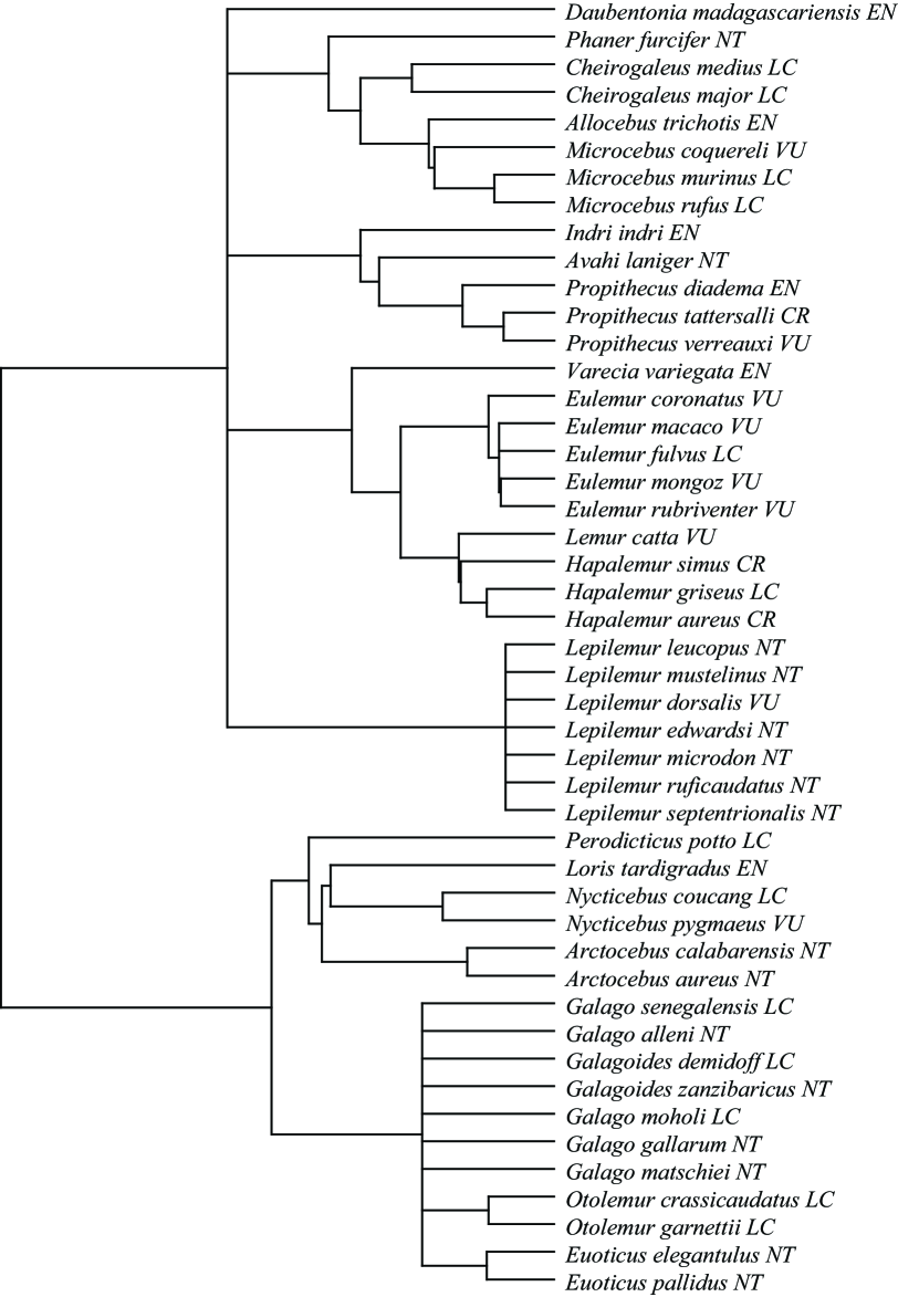
The bivariate correlation between the metrics is high (0.94). Both measures chose the Aye-Aye ( ) as the most important species, followed by . Interestingly, the three most highly ranked species under current conservation policy (the critically endangered lemurs , , ) are nested well up in the tree (Figure 2) such that none of them were chosen in the top ten for either SV or HED. If we compare the rest of the rankings for these two metrics, the largest single difference is for the two species: they rank twelfth under SV (being relatively isolated on the tree), but only twenty-sixth under HED: because neither is severely threatened, the chances are good that their common path will persist.
Both measures are very heavily influenced by the pendant edge () length of the focal species (with correlations vs. SV=0.94, and vs. HED=0.98). is always part of the marginal increase to , while interior nodes are most likely represented with high probability, especially for larger and more balanced trees. is, however, a poor predictor of HED for , for , and for (Figure 2). The first two groups contain the three most endangered species, increasing the value of close relatives. is an isolated genus, and ’s sister species is listed as vulnerable ( ). Likewise for - although it has close relatives and so a short PE, these relatives are at high risk of extinction, which increases its value; this is what we saw with species in figure 1.
4.1 Incorporating the focal taxon’s extinction risk (HEDGE scores)
The effect of close relatives’ risk status on one’s own value is precisely the strength of the HED approach. However, the fact that the extinction risk of other species affects a focal species, but its own risk does not is somewhat counter-intuitive. We address this by showing how it is possible to write the HED index as the sum of two terms each of which takes into account the extinction risk of the focal species. To describe this further, let be the random variable which takes the value if the focal species survives (at the future time under consideration) and which otherwise takes the value of the emptyset (i.e. ) if goes extinct.
Let
where, as before is the random subset of species in that survive. In words, is the increase in the expected PD score if we condition on the event that species survives.
Similarly, let
In words, is the decrease in the expected PD score if we condition on the event that species becomes extinct. The following result describes how to compute these two indices easily from the HED index, and verifies that they add together to give the HED index (its proof is given in the Appendix).
Theorem 4.1
-
(i)
,
-
(ii)
,
-
(iii)
.
The approach of assigning a value to a species which is a function of its phylogenetic distinctiveness and its extinction probability has been referred to as ‘expected loss’ by Redding and Mooers (2006) and, more evocatively, an ‘EDGE’ score (Evolutionarily Distinct and Globally Endangered) by Isaac et al. (2007).
In the same spirit we will call and (which extend our HED index ) HEDGE (heightened evolutionary distinctiveness and globally endangered) scores. The HEDGE score is more relevant when evaluating actions that might save species, whereas the HEDGE score is appropriate when evaluating actions that might cause the extinction of species (such as building a dam).
One potential advantage of HED and HEDGE over previous scores is their flexibility in designing conservation scenarios. So for instance, we can choose IUCN-ranked species for which conservation is cheap and/or already partially successful, set their to 0, and see how rankings of other species change. Alternatively, we might want to increase the to 1.0 for certain species to see how others are affected.
Most generally, HED and HEDGE could be incorporated in an assessment of species value that included many factors besides risk and future contribution, e.g. the ecological, distributional and aesthetic values enumerated by Avise (2005), and the costs of recovery and probability of its success.
5 Appendix: Proofs of theorems.
Proof of Theorem 3.1
First observe that the only edge lengths that contribute to are those from the set .
Consequently, for the random set of surviving species of we have
where is the indicator random variable that takes the value precisely if is not an edge of the subtree of connecting the taxa in and the root of ; since this is the only situation for which lies in the subtree of connecting but not in the subtree of connecting .
Thus, by linearity of expectation,
and since takes the values and , . Thus,
Now, the event ‘’ occurs precisely if none of the elements in survive, and this latter event has probability . Substituting this into the previous equation establishes the theorem.
Proof of Theorem 3.2
For and the random subset , we have
where is the indicator random variable taking the value precisely if consists of no elements of and at least one element of .
Thus,
and by the independence assumption
and so
as claimed.
Proof of Theorem 4.1
By definition , and so .
Now we can write the unconditional expectation as the weighted sum of conditional expectations and so
Parts (i) and (ii) now follow by applying these equations (and the linearity of expectation) to the definitions of and . Part (iii) follows directly from parts (i) and (ii).
6 Acknowledgments
This research was supported by a grant from the Marsden Fund, New Zealand to MS and AOM. AOM received additional support from NSERC Canada and the Institute for Advanced Study, Berlin. We thank Dave Redding, Klaas Hartmann, and Andy Purvis for discussion.
References
- (1) Altschul, S. F., and D. J. Lipman. 1990. Equal animals. Nature 348:493–494.
- (2) Avise J.C. 2005. Phylogenetic units and currencies above and below the species level. Pages 77-100 in Purvis A, Gittleman JL, and Brooks T, eds. Phylogeny and conservation Cambridge University Press, Cambridge, UK.
- (3) Cousins, S.H. 1991. Species diversity measurement: choosing the right index. Trends in Ecology and Evolution 6:190–192.
- (4) Faith, D.P. 1992. Conservation evaluation and phylogenetic diversity. Biological Conservation 61:1-10.
- (5) Haake, C-J, Kashiwada, A., and F.E. Su. 2005. The shapley value of phylogenetic trees. IMW Working Paper 363 (363). ArXiv (q-bio.QM/0506034)
- (6) Hartmann, K. and M. Steel. 2007. Phylogenetic diversity: from combinatorics to ecology. Forthcoming. In O. Gascuel and M. Steel eds. Reconstruction evolution: New mathematical and computational advances. Oxford University Press.
- (7) Isaac, N.J.B., Turvey, S.T., Collen, B., Waterman, C., and J.E.M. Baillie. 2007. Mammals on the EDGE: conservation priorities based on threat and phylogeny. PLoS ONE 2(3): e296.
- (8) May, R.M. 1990. Taxonomy as Destiny. Nature 347:129–130.
- (9) Mooers, A.O. and S.B. Heard. 1997. Inferring process from phylogenetic tree shape. Quarterly Review of Biology 72:31-54.
- (10) Myers, N.,Mittermeier, R. A., Mittermeier, C. G., da Fonseca, G. A. B., and J. Kent. 2000. Biodiversity hotspots for conservation priorities. Nature 403:853–858.
- (11) Pavoine, S., Ollier, S., and D. Pontier. 2005. Measuring diversity from dissimilarities with Rao’s quadratic entropy: Are any dissimilarities suitable? Theoretical Population Biology 67:231–239.
- (12) Pavoine, S., S. Ollier, and A.B. Dufour. 2005. Is the originality of a species measurable? Ecology Letters 8:579-586.
- (13) Redding, D.W. and A.O. Mooers. 2006. Incorporating evolutionary measures into conservation prioritization. Conservation Biology 20:1670-1678.
- (14) SARA. 2002. Bill C-5, An Act respecting the protection of wildlife species at risk in Canada. Government of Canada, Ottawa.
- (15) Shapley, L.S. 1953. A value for n-person games. Annals of Mathematical Studies 28:307-317.
- (16) Vos, R.A., and A.O. Mooers. 2004. Reconstructing divergence times for supertrees: a molecular approach. Pages 281-299 in O. R. P. Bininda-Emonds, ed. Phylogenetic supertrees: combining information to reveal the Tree of Life. Kluwer Academic Press, 765. Dordrecht.
- (17) Vos, R. 2006. Inferring large phylogenies: the big tree problem. PhD. Thesis, Simon Fraser University.