Height-bounded Lempel-Ziv encodings

Dictionary compressors are a family of algorithms that produce compressed representations of input strings essentially as sequences of copy and paste operations. These representations are widely used in general compression tools such as gzip and LZ4, and have also received much recent attention since they are especially effective for highly repetitive data sets, such as versioned documents and pangenomes [23].

A desirable operation to support on compressed data is that of random access to arbitrary positions in the original data. Access should be supported without decompressing the data in its entirety, and ideally by decompressing little else than the sought positions. Recent years have seen intense research on the access problem in the context of dictionary compression, most notably for grammar compressors (SLPs) and Lempel-Ziv (LZ)-like schemes. The general approach is to impose structure on the output of the compressor and in doing so add small amounts of information to support fast queries. While LZ77 [34] is known to be theoretically and practically one of the smallest compressed representations that can be computed efficiently, a long-standing question is whether $O(\polylog(n))$ time access can be achieved with a data structure using $O(z)$ space [23], where $z$ is the size of the LZ77 parsing.

In an LZ-like compression scheme, the input string $T$ of length $n$ is parsed into $z^{\prime}\leq n$ phrases (substrings of $T$), where each phrase is of length $1$, or, is a phrase of length at least $2$ which has a previous occurrence. Each phrase can be encoded by a pair $(\ell,s)$, where $\ell\geq 1$ is the length of the phrase, and $s$ is the symbol representing the phrase if $\ell=1$, or otherwise, a position of a previous occurrence (source) of the phrase. A greedy left-to-right algorithm that takes the longest prefix of the remaining string that can be a phrase leads to the aforementioned LZ77 parsing. An LZ-like encoding of a string induces a referencing forest, where each position of the string is a node, phrases of length 1 are roots of a tree in the forest, and the parent of all other positions are induced by the previous occurrence of the phrase it is contained in. The principle hurdle to support fast access to an arbitrary symbol $T[i]$ from an LZ-like parsing is to trace the symbol to a root in the referencing forest. For LZ77, the height of the referencing forest can be $\Theta(n)$.

We first consider modifying the definition of the height of the referencing forest under some conditions, by implicitly rerouting edges. Consider the case of a unary string $T=\mathtt{a}^{n}$ and LZ-like encoding $(1,\mathtt{a}),(n-1,1)$. The straightforward definition above gives a height of $n-1$ for position $n$. This is a result of the second phrase being self-referencing, i.e., the phrase overlaps with its referenced occurrence, and each position references its preceding position. An important observation is that self-referencing phrases are periodic; in particular a self-referencing phrase starting at position $b_{i}$ with source $s_{i}$ has period $b_{i}-s_{i}$. Due to this periodicity, any position in the phrase can refer to an appropriate position in $T[s_{i}..b_{i})$.

More formally, let $\mathcal{E}=(\ell_{1},s_{1}),\ldots,(\ell_{z^{\prime}},s_{z^{\prime}})$ be an LZ-like encoding of $T$. For any position $i$, let $b_{j}$ be the starting position of the phrase $(\ell_{j},s_{j})$ such that $b_{j}\leq i<b_{j}+\ell_{j}$. Then, $T[i]=s_{j}$ if $\ell_{j}=0$, and $T[i]=T[s_{j}+(i-b_{j})]=T[s_{j}+((i-b_{j})\bmod(b_{j}-s_{j}))]$ otherwise.

We define the height $0pt_{\mathcal{E}}(i)$ of position $i$ by an encoding $\mathcal{E}$ as

The subscript will be omitted if the underlying encoding considered is clear. Since $j$ can be computed using a predecessor query on the set of phrase starting positions, $T[i]$ can be computed using $O(0pt(i)Q(z))$ time using a data structure of size $O(z)$, where $Q(z)$ is the time required for predecessor queries on $z$ elements in $[1,n]$ using $O(z)$ space. $Q(z)$ is $O(\log n)$ using a simple binary search, and faster using more sophisticated methods [21].

For example, for the encoding $(1,\mathtt{a}),(1,\mathtt{a}),(1,\mathtt{b}),(3,2),(1,\mathtt{c}),(4,3)$ of string $\mathtt{aababacbaba}$, the heights are: $0,0,0,1,1,1,0,1,2,2,2$. Notice that the phrase $(3,2)$ that starts at position $4$, representing $\mathtt{aba}$ is self-referencing, and the height of the last position in the phrase (position 6) is $1$, since it is defined to reference position $2=2+(6-4)\bmod(6-4)$. We note that even with this modified definition, the height of the optimal LZ-like encoding (LZ77) can be $\Theta(n)$. See Appendix A in Appendix A.

In order to bound the worstcase query time complexity for access operations, we consider LZ-like encodings with bounded height. An $h$-bounded LZ-like encoding is an LZ-like encoding where $\max\{0pt(i)\mid i\in[1,n]\}\leq h$.

There are many ways one could enforce such a height restriction. Unfortunately, finding the smallest such encoding was very recently shown to be NP-hard by Cicalese and Ugazio [8]. Therefore, we propose several greedy heuristics to compute $h$-bounded LZ-like encodings. Given an encoding for $T[1..b_{j})$ (which defines $0pt(i)$ for any $i\in[1,b_{j})$), the next phrase $(\ell_{j},s_{j})$ starting at position $b_{j}$ is defined as follows.

LZHB1

$\ell_{j}$ is the largest value such that $T[s_{j}..s_{j}+\ell_{j})$ satisfies the height constraint, where $s_{j}=\mathrm{lmocc}_{T}(b_{j},\mathrm{lpf}_{T}(b_{j}))$, i.e., the leftmost occurrence of the longest previously occurring factor at position $b_{j}$.

LZHB2

$\ell_{j}$ is the largest value such that for all $1\leq\ell^{\prime}\leq\ell_{j}$, the leftmost occurrence of $T[b_{j}..b_{j}+\ell^{\prime})$ satisfies the height constraint. $s_{j}$ is the leftmost occurrence of $T[b_{j}..b_{j}+\ell_{j})$.

LZHB3

$\ell_{j}$ is the largest value such that for all $1\leq\ell^{\prime}\leq\ell_{j}$, there exists some previous occurrence of $T[b_{j}..b_{j}+\ell^{\prime})$ that satisfies the height constraint. $s_{j}$ is the leftmost occurrence of $T[b_{j}..b_{j}+\ell_{j})$ that satisfies the height constraint.

Note that for all variations, $\ell_{j}=1$ if there is no occurrence of $T[b_{j}]$ that satisfies the corresponding conditions described above, in which case, $s_{j}=T[b_{j}]$.

We note that LZHB1 corresponds to the baseline algorithm BATLZ2 in [18]. LZHB3 essentially corresponds to greedy-BATLZ in [18] as well, but greedy-BATLZ does not require that the occurrence is leftmost. The difference between LZHB2 and LZHB3 lies in the priority of the choice of the leftmost occurrence and when to check the height constraint. LZHB2 greedily extends the prefix, checking each time whether its leftmost occurrence satisfies the height constraint. LZHB3 finds the leftmost occurrence out of the longest prefix that can satisfy the height constraint. Note that when the height is unbounded, the size of all three variants will be equivalent to the regular LZ77 parsing.

We show that LZHB1 and LZHB2 can be computed in $O(n)$ time and space for linearly-sortable alphabets, and LZHB3 can be computed online in $O(n\log\sigma)$ time and $O(n)$ space for general ordered alphabets.

We also propose a new encoding of LZ-like parsings that re-routes edges of the implicit referencing forest in an attempt to further reduce the heights, again using periodicity. In the case of self-referencing phrases, our definition of height in Equation (1) utilized the fact that self-referencing phrases implies a period $b_{j}-s_{j}$ in the phrase. Using this period, we could re-route the parents of all positions inside the phrase to the first period in the previous occurrence of the phrase, which is outside the phrase. Here, we make two further observations: 1) since the referenced substring is the first period of the phrase, we could extended the phrase for free while the period continues, possibly making the phrase longer, and 2) the referenced substring could have a previous occurrence further to the left, which should tend to have shorter heights. Therefore, if we were to store the period of the phrase explicitly, this could be applied to and benefit all periodic phrases, self-referencing or not.

Specifically then, under this scheme, a phrase with period $1$ can be encoded as the triple $(\ell,c,1)$, where $c$ is a symbol, and a phrase with period $p\geq 2$ can be encoded as the triple $(\ell,s,p)$, where $\ell\geq p$ is the length of the phrase with period $p\geq 2$, and $s$ is a previous occurrence of the length-$p$ prefix of the phrase. We will call such an encoding, a modified LZ-like encoding. For example, $(2,\mathtt{a},1),(1,\mathtt{b},1),(3,2,2),(1,\mathtt{c},1),(4,3,2)$ would be a modified LZ-like encoding for the string $\mathtt{aababacbaba}$.

The implicit referencing forest and heights of the modified LZ-like encoding can be defined analogously: a position $i$ in the $j$th phrase $(\ell_{j},s_{j},p_{j})$ that begins at position $b_{j}$, i.e., $b_{j}\leq i<b_{j}+\ell_{j}$, will reference position $s_{j}+((i-b_{j})\bmod p_{j})\bmod(b_{j}-s_{j})$, where the second $\bmod$ is to deal with the case where the occurrence of the prefix period is self-referencing. For the above example, the heights are: $0,0,0,1,1,1,0,1,2,1,2$.

A greedy left-to-right algorithm computes the $j$th phrase $(\ell_{j},s_{j},p_{j})$ starting at $b_{j}$ as:

LZHB4

$\ell_{j}$ is the largest value such that $T[b_{j}..b_{j}+\ell_{j})$ has period $1$, or, for all $1\leq\ell^{\prime}\leq\ell_{j}$, there exists some previous occurrence of $T[b_{j}..b_{j}+p^{\prime})$ that satisfies the height constraint, where $p^{\prime}$ is the minimum period of $T[b_{j}..b_{j}+\ell^{\prime})$. $s_{j}$ is the leftmost occurrence of $T[b_{j}..b_{j}+\ell_{j})$ that satisfies the height constraint, and $p_{j}$ is the minimum period of $T[b_{j}..b_{j}+\ell_{j})$.

Here, we consider the strength of height bounded encodings as repetitiveness measures [23]. Denote by $\hat{z}_{\mathit{HB}(h)}$, the optimal (smallest) LZHB encoding whose height is at most $h$. It easily follows that $\hat{z}_{\mathit{HB}(h)}$ is monotonically non-increasing in $h$, i.e., for any $h\leq h^{\prime}$, it holds that $\hat{z}_{\mathit{HB}(h)}\geq\hat{z}_{\mathit{HB}(h^{\prime})}$. We will also denote by $\hat{\tilde{z}}_{\mathit{HB}(h)}$, the optimal modified LZ-like encoding whose height is at most $h$.

A first, and obvious, observation is that if the height is allowed to grow to $n$, then the size of the height-bounded encoding and the LZ parsing are equivalent. {observation} $\hat{z}_{\mathit{HB}(n)}=z$.

It is also interesting to note height-bounded and run-length encodings can be related: {observation} $\hat{\tilde{z}}_{\mathit{HB}(0)}$ is equivalent to the run-length encoding.

The following relation between $\hat{z}_{\mathit{HB}(h)}$ and the smallest size $\hat{g}_{\mathrm{rl}}$ of RLSLPs (SLPs with run-length rules) and $\hat{g}_{it(d)}$ of ISLPs [26] can be shown.

When there is no height constraint, LZHB3 is equivalent to LZ77 and thus gives an optimal LZ-like parsing. For modified LZ-like encodings with no height contraints, LZHB4 can be worse than optimal. For example, for the string $\mathtt{abaxabcdababca}$, greedy gives $\mathtt{a}|\mathtt{b}|\mathtt{a}|\mathtt{x}|\mathtt{ab}|\mathtt{c}|\mathtt{d}|\mathtt{abab}|\mathtt{c}|\mathtt{a}$ while $\mathtt{a}|\mathtt{b}|\mathtt{a}|\mathtt{x}|\mathtt{ab}|\mathtt{c}|\mathtt{d}|\mathtt{ab}|\mathtt{abca}$ is a slightly smaller parsing. However, we can show that the greedy algorithm has an approximation ratio of at most $2$.

We have developed prototype implementations of our algorithms described above, in C++. Since Lipták et al. [18] have already demonstrated the effectiveness and superiority of greedy-BATLZ and greedier-BATLZ (which correspond to LZHB3 and the greedier LZHB3) compared to the baselines and that the height can be reduced without increasing the size of the parse too much, our experiments here focus on the performance of our algorithms LZHB3 and LZHB4 in comparison with greedy-BATLZ and greedier-BATLZ. For the BAT-LZ variants, we use the code provided by Lipt’ak et al.³³3Available at: https://github.com/fmasillo/BAT-LZ. with slight modifications to fit our test environment. Our implementations for LZHB3 and LZHB4 are available at https://github.com/dscalgo/lzhb/.

Experiments were conducted on a system with dual AMD EPYC 9654 2.4GHz processors and 768GB RAM running RedHat Linux 8. We use the Real subset of the repetitive corpus⁴⁴4https://pizzachili.dcc.uchile.cl/repcorpus.html.

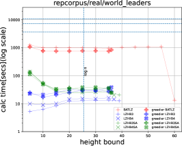
Figure 2 shows the running times for various height constraints of the BAT-LZ variants as well as LZHB3, LZHB3SA, LZHB4, and LZHB4SA, and their greedier versions, where the suffix SA denotes the suffix array implementation. Although greedy-BATLZ is fast when there is no height constraint, its performance seems to diminish rapidly when a height constraint is set. Interestingly, greedier-BATLZ seemed to run faster than greedy-BATLZ. We observe that all versions of our LZHB3 and LZHB4 implementation outperform greedy-BATLZ and greedier-BATLZ by a large margin. For the greedier variants, the running times increase as the height constraint decreases. This is because stricter height constraints generally lead to shorter phrase lengths and therefore increases $z^{\prime}$ and $\mathit{occ}$. This becomes more apparent in the suffix array versions, perhaps because the $n$ in the $O(\log n)$ factor for finding the suffix array range is actually the size of the range considered, which becomes larger for shorter pharses.

Figure 3 shows the memory usage of the above mentioned implementations. The memory usage for LZHB3 and LZHB4 (the suffix tree versions) are smallest for small heights, because smaller height constraints imply that many paths in the suffix tree become truncated. On the other hand, the memory usage is the highest for larger heights. Memory usage for the other versions is unaffected by the height constraint. LZHB3SA and LZHB4SA are always superior to greedy-BATLZ, and the same can be said for the greedier versions and their counterparts.

In summary, our suffix array implementations are always faster and use less memory than their BATLZ counterparts, with the exception of greedy-BATLZ with no height constraints.

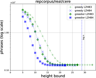
Figure 4 shows the sizes of the phrases of LZHB3, LZHB4 and their greedier versions⁵⁵5We also ran experiments for LZ End parsing, but do not include results in the figures because they distort the plots. We include statistics for LZ End in Table 1 in the Appendix.. Although a phrase of the modified LZ-like encoding is slightly larger than the traditional LZ-like encoding since it includes the period, we can see that a much smaller encoding with the same height, which can more than compensate for this increase, can be obtained in some cases. This seemed to be prominent for cere, para, and Escherichia_Coli, which are all DNA.

We have introduced new variants of LZ-like encodings that directly focus on supporting random access to the underlying data. We also proposed a modified LZ-like encoding, which naturally connects the run-length encoding ($h=0$), and LZ77 ($h=n$). We described linear time algorithms for several greedy variants of such encodings, as well as how to adapt them to support the greedier heuristic. We showed that our algorithms are faster both theoretically and practically, compared to contemporaneously proposed algorithms by Lipták et al. [18]. We also showed some relations between height-bounded encodings and existing repetitiveness measures. In particular, we have shown that the optimal LZ-like encoding with a height constraint of $O(\log n)$, is one of the asymptotically smallest repetitiveness measures achieving fast (i.e., $O(\polylog(n))$-time) access.

There are numerous avenues future work could take. An obvious next step is to engineer actual random-access data structures from height-bounded encodings, which our experiments presented here indicate should be competitive with current state-of-the-art methods. Also, other heuristics for reducing the height while retaining the small size should be explored.

From a theoretical perspective, a natural open problem is whether we can remove the $\log\sigma$ factor from the running times of LZHB3 and LZHB4. The biggest open problem we leave is whether better bounds on the size of height-bounded encodings can be established. Cicalese and Ugazio show that $\hat{z}_{\mathit{HB}(h)}=O(z)$ [8] cannot be achieved for costant $h$. We note that since there exist linear sized data structures that can answer predecessor queries for a set of values in the range $[1,n]$ in $O(\log\log n)$ time [33], even better lower bounds on the height for which $\hat{z}_{\mathit{HB}(h)}=O(z)$ can be shown by using access time lower bound results of Verbin and Yu [31]. However, these do not rule out $O(\polylog(n))$ height. Can we balance the height (achieve $O(\polylog(n))$ height) of an LZ-like encoding or a modified LZ-like encoding, by only increasing the size by a constant factor?

References

- [1] Mohamed Ibrahim Abouelhoda, Stefan Kurtz, and Enno Ohlebusch. Replacing suffix trees with enhanced suffix arrays. J. Discrete Algorithms, 2(1):53–86, 2004. doi:10.1016/S1570-8667(03)00065-0.
- [2] Djamal Belazzougui, Dmitry Kosolobov, Simon J. Puglisi, and Rajeev Raman. Weighted ancestors in suffix trees revisited. In Pawel Gawrychowski and Tatiana Starikovskaya, editors, 32nd Annual Symposium on Combinatorial Pattern Matching, CPM 2021, July 5-7, 2021, Wrocław, Poland, volume 191 of LIPIcs, pages 8:1–8:15. Schloss Dagstuhl - Leibniz-Zentrum für Informatik, 2021. URL: https://doi.org/10.4230/LIPIcs.CPM.2021.8, doi:10.4230/LIPICS.CPM.2021.8.
- [3] Jon Louis Bentley and Derick Wood. An optimal worst case algorithm for reporting intersections of rectangles. IEEE Trans. Computers, 29(7):571–577, 1980. doi:10.1109/TC.1980.1675628.
- [4] Jean Berstel and Alessandra Savelli. Crochemore factorization of sturmian and other infinite words. In Rastislav Kralovic and Pawel Urzyczyn, editors, Mathematical Foundations of Computer Science 2006, 31st International Symposium, MFCS 2006, Stará Lesná, Slovakia, August 28-September 1, 2006, Proceedings, volume 4162 of Lecture Notes in Computer Science, pages 157–166. Springer, 2006. doi:10.1007/11821069\_14.
- [5] Philip Bille, Travis Gagie, Inge Li Gørtz, and Nicola Prezza. A separation between RLSLPs and LZ77. J. Discrete Algorithms, 50:36–39, 2018. URL: https://doi.org/10.1016/j.jda.2018.09.002, doi:10.1016/J.JDA.2018.09.002.
- [6] Moses Charikar, Eric Lehman, Ding Liu, Rina Panigrahy, Manoj Prabhakaran, Amit Sahai, and Abhi Shelat. The smallest grammar problem. IEEE Trans. Inf. Theory, 51(7):2554–2576, 2005. doi:10.1109/TIT.2005.850116.
- [7] Bernard Chazelle. A functional approach to data structures and its use in multidimensional searching. SIAM J. Comput., 17(3):427–462, 1988. doi:10.1137/0217026.
- [8] Ferdinando Cicalese and Francesca Ugazio. On the complexity and approximability of bounded access Lempel Ziv coding. CoRR, abs/2403.15871, 2024. URL: https://doi.org/10.48550/arXiv.2403.15871, arXiv:2403.15871, doi:10.48550/ARXIV.2403.15871.
- [9] Sorin Constantinescu and Lucian Ilie. The Lempel–Ziv complexity of fixed points of morphisms. SIAM J. Discret. Math., 21(2):466–481, 2007. doi:10.1137/050646846.
- [10] Maxime Crochemore, Lucian Ilie, Costas S. Iliopoulos, Marcin Kubica, Wojciech Rytter, and Tomasz Walen. Computing the longest previous factor. Eur. J. Comb., 34(1):15–26, 2013. URL: https://doi.org/10.1016/j.ejc.2012.07.011, doi:10.1016/J.EJC.2012.07.011.
- [11] Martin Farach. Optimal suffix tree construction with large alphabets. In 38th Annual Symposium on Foundations of Computer Science, FOCS ’97, Miami Beach, Florida, USA, October 19-22, 1997, pages 137–143. IEEE Computer Society, 1997. doi:10.1109/SFCS.1997.646102.
- [12] Johannes Fischer. Inducing the lcp-array. In Frank Dehne, John Iacono, and Jörg-Rüdiger Sack, editors, Algorithms and Data Structures - 12th International Symposium, WADS 2011, New York, NY, USA, August 15-17, 2011. Proceedings, volume 6844 of Lecture Notes in Computer Science, pages 374–385. Springer, 2011. doi:10.1007/978-3-642-22300-6\_32.
- [13] Dan Gusfield. Algorithms on Strings, Trees, and Sequences: Computer Science and Computational Biology. Cambridge University Press, 1997. doi:10.1017/CBO9780511574931.
- [14] Dominik Kempa and Barna Saha. An upper bound and linear-space queries on the LZ-end parsing. In Joseph (Seffi) Naor and Niv Buchbinder, editors, Proceedings of the 2022 ACM-SIAM Symposium on Discrete Algorithms, SODA 2022, Virtual Conference / Alexandria, VA, USA, January 9 - 12, 2022, pages 2847–2866. SIAM, 2022. doi:10.1137/1.9781611977073.111.
- [15] Donald E. Knuth, James H. Morris Jr., and Vaughan R. Pratt. Fast pattern matching in strings. SIAM J. Comput., 6(2):323–350, 1977. doi:10.1137/0206024.
- [16] Sebastian Kreft and Gonzalo Navarro. LZ77-like compression with fast random access. In James A. Storer and Michael W. Marcellin, editors, 2010 Data Compression Conference (DCC 2010), 24-26 March 2010, Snowbird, UT, USA, pages 239–248. IEEE Computer Society, 2010. doi:10.1109/DCC.2010.29.
- [17] Sebastian Kreft and Gonzalo Navarro. On compressing and indexing repetitive sequences. Theor. Comput. Sci., 483:115–133, 2013. URL: https://doi.org/10.1016/j.tcs.2012.02.006, doi:10.1016/J.TCS.2012.02.006.
- [18] Zsuzsanna Lipták, Francesco Masillo, and Gonzalo Navarro. BAT-LZ out of hell. CoRR, abs/2403.09893, 2024. To appear at CPM ’24. URL: https://doi.org/10.48550/arXiv.2403.09893, arXiv:2403.09893, doi:10.48550/ARXIV.2403.09893.
- [19] Udi Manber and Gene Myers. Suffix arrays: A new method for on-line string searches. In David S. Johnson, editor, Proceedings of the First Annual ACM-SIAM Symposium on Discrete Algorithms, 22-24 January 1990, San Francisco, California, USA, pages 319–327. SIAM, 1990. URL: http://dl.acm.org/citation.cfm?id=320176.320218.
- [20] S. Muthukrishnan. Efficient algorithms for document retrieval problems. In David Eppstein, editor, Proceedings of the Thirteenth Annual ACM-SIAM Symposium on Discrete Algorithms, January 6-8, 2002, San Francisco, CA, USA, pages 657–666. ACM/SIAM, 2002. URL: http://dl.acm.org/citation.cfm?id=545381.545469.
- [21] G. Navarro and J. Rojas-Ledesma. Predecessor search. ACM Computing Surveys, 53(5):article 105, 2020.
- [22] Gonzalo Navarro. Compact Data Structures - A Practical Approach. Cambridge University Press, 2016.
- [23] Gonzalo Navarro. Indexing highly repetitive string collections, part I: repetitiveness measures. ACM Comput. Surv., 54(2):29:1–29:31, 2022. doi:10.1145/3434399.
- [24] Gonzalo Navarro, Carlos Ochoa, and Nicola Prezza. On the approximation ratio of ordered parsings. IEEE Trans. Inf. Theory, 67(2):1008–1026, 2021. doi:10.1109/TIT.2020.3042746.
- [25] Gonzalo Navarro, Francisco Olivares, and Cristian Urbina. Balancing run-length straight-line programs. In Diego Arroyuelo and Barbara Poblete, editors, String Processing and Information Retrieval - 29th International Symposium, SPIRE 2022, Concepción, Chile, November 8-10, 2022, Proceedings, volume 13617 of Lecture Notes in Computer Science, pages 117–131. Springer, 2022. doi:10.1007/978-3-031-20643-6\_9.
- [26] Gonzalo Navarro and Cristian Urbina. Iterated straight-line programs. In Proc. LATIN 2024, Lecture Notes in Computer Science, 2024.
- [27] Takaaki Nishimoto, Tomohiro I, Shunsuke Inenaga, Hideo Bannai, and Masayuki Takeda. Fully dynamic data structure for LCE queries in compressed space. In 41st International Symposium on Mathematical Foundations of Computer Science, MFCS 2016, August 22-26, 2016 - Kraków, Poland, volume 58 of LIPIcs, pages 72:1–72:15. Schloss Dagstuhl - Leibniz-Zentrum für Informatik, 2016.
- [28] Wojciech Plandowski and Wojciech Rytter. Application of Lempel-Ziv encodings to the solution of words equations. In Kim Guldstrand Larsen, Sven Skyum, and Glynn Winskel, editors, Automata, Languages and Programming, 25th International Colloquium, ICALP’98, Aalborg, Denmark, July 13-17, 1998, Proceedings, volume 1443 of Lecture Notes in Computer Science, pages 731–742. Springer, 1998.
- [29] Yohei Ueki, Diptarama, Masatoshi Kurihara, Yoshiaki Matsuoka, Kazuyuki Narisawa, Ryo Yoshinaka, Hideo Bannai, Shunsuke Inenaga, and Ayumi Shinohara. Longest common subsequence in at least k length order-isomorphic substrings. In Bernhard Steffen, Christel Baier, Mark van den Brand, Johann Eder, Mike Hinchey, and Tiziana Margaria, editors, SOFSEM 2017: Theory and Practice of Computer Science - 43rd International Conference on Current Trends in Theory and Practice of Computer Science, Limerick, Ireland, January 16-20, 2017, Proceedings, volume 10139 of Lecture Notes in Computer Science, pages 363–374. Springer, 2017. doi:10.1007/978-3-319-51963-0\_28.
- [30] Esko Ukkonen. On-line construction of suffix trees. Algorithmica, 14(3):249–260, 1995. doi:10.1007/BF01206331.
- [31] Elad Verbin and Wei Yu. Data structure lower bounds on random access to grammar-compressed strings. In Johannes Fischer and Peter Sanders, editors, Combinatorial Pattern Matching, 24th Annual Symposium, CPM 2013, Bad Herrenalb, Germany, June 17-19, 2013. Proceedings, volume 7922 of Lecture Notes in Computer Science, pages 247–258. Springer, 2013. doi:10.1007/978-3-642-38905-4\_24.
- [32] Peter Weiner. Linear pattern matching algorithms. In 14th Annual Symposium on Switching and Automata Theory, Iowa City, Iowa, USA, October 15-17, 1973, pages 1–11. IEEE Computer Society, 1973.
- [33] Dan E. Willard. Log-logarithmic worst-case range queries are possible in space theta(n). Inf. Process. Lett., 17(2):81–84, 1983. doi:10.1016/0020-0190(83)90075-3.
- [34] Jacob Ziv and Abraham Lempel. A universal algorithm for sequential data compression. IEEE Trans. Inf. Theory, 23(3):337–343, 1977. doi:10.1109/TIT.1977.1055714.
Appendix A Ommitted Proofs
The height of the optimal LZ-like encoding (LZ77) can be .
Proof A.1.
Consider the height of in the string:
It is not difficult to see each will reference the closest previously occurring .
See 5.1
Proof A.2.
It is known that a given RLSLP can be balanced, i.e., transformed into another RLSLP whose parse tree height is , without changing the asymptotic size of the RLSLP [25].
Theorem A.3 (Theorem 1 in [25]).
Given an RLSLP generating a string , it is possible to construct an equivalent balanced RLSLP of size , in linear time, with only rules of the form ,, and , where is a terminal, and are variables, and .
Given an RLSLP with parse tree height , a partial parse tree of the RLSLP, as defined in Theorem 5 of [24], can be obtained. Based on this partial parse tree, it is possible to obtain an LZ-like encoding of size at most that of the run-length grammar. The height of the LZ-like encoding corresponds to the height of the parse tree, and thus is -bounded. Since, from Theorem A.3, we can obtain a grammar of size with height , we have that the size of an optimal -bounded LZ-like encoding will have size at most , where is a constant incurred by the height of the balanced RLSLP obtained from balancing the optimal run-length grammar.
See 5.2
Proof A.4.
The proof follows similar arguments to those of Bille et al. [5]. In their proof, they consider a string (originally used by Charikar et al. [6])
where denotes the length- prefix of the Thue-Morse word, are distinct symbols, and is an integer sequence where is the largest of the , , and show that the integers can be chosen so that the smallest RLSLP for has size . They further observe that the size of an LZ77 parsing of the length- prefix of the Thue-Morse word is [4, 9]. Since is the largest of the ’s, the size of the LZ77 parsing of is for this class of strings.
Now, observe that the height, as defined in Equation (1), of an LZ-like encoding with size is , since any position in a phrase references a position in a previous phrase. Therefore, we have that for some , as well, thus showing that .
Since Thue-Morse words are cube-free, the extra rules in the iterated SLPs do not improve the asymptotic size compared to RLSLPs, and thus, as shown in Lemma 3 of [26], for this family of strings. Therefore, we have .
See 5.3
Proof A.5.
It is obvious that . We first claim . This can be seen from the fact that a phrase that starts at position in (the greedy) LZHB4 is at least as long as , and so any LZHB phrase must extend at least to the end of the LZ77 phrase it starts in. Thus, for each LZHB phrase, we can assign a distinct LZ77 phrase (the LZ77 phrase it starts in), and therefore the number of LZHB4 phrases cannot be more than the number of LZ77 phrases.
Next, we claim for any modified LZ-like encoding with no height constraints, whose size is denoted by . This can be seen from the fact that a given phrase in a modified LZ-like encoding can contain at most two LZ77 phrases that start in it. Let be a phrase in the modified LZ-like encoding starting at position , whose minimum period is and is a prefix of . Since there is a previous occurrence of , the first LZ77 phrase that starts in the LZHB phrase must extend to at least the end of the first . Since there is a previous occurrence of any suffix of , the next LZ77 phrase will extend at least to the end of the LZHB phrase. The theorem follows from the above arguments, using for .
Appendix B Pseudo codes
Appendix C More results of computational experiments