Helical superfluid in a frustrated honeycomb Bose-Hubbard model
Abstract
We study a “helical” superfluid, a nonzero-momentum condensate in a frustrated bosonic model. At mean-field Bogoliubov level, such a novel state exhibits “smectic” fluctuation that are qualitatively stronger than that of a conventional superfluid. We develop a phase diagram and compute a variety of its physical properties, including the spectrum, structure factor, condensate depletion, momentum distribution, all of which are qualitatively distinct from that of a conventional superfluid. Interplay of fluctuations, interaction and lattice effects gives rise to the phenomenon of order-by-disorder, leading to a crossover from the smectic superfluid regime to the anisotropic XY superfluid phase. We complement the microscopic lattice analysis with a field theoretic description for such a helical superfluid, which we derive from microscopics and justify on general symmetry grounds, reassuringly finding full consistency. Possible experimental realizations are discussed.
I Introduction
Frustrated systems exhibit novel emergent phenomena as they often host extensive degeneracy that is sensitive to even weak perturbations Moessner and Chalker (1998); Balents (2010). This manifests itself in rich low-temperature phenomenology, as in the frustrated magnetism, which commonly remains disordered down to temperatures low compared to the Curie-Weiss temperature set by the exchange interaction Ramirez et al. (1990); Gaulin et al. (1992); Ramirez (1994); Uemura et al. (1994); Dunsiger et al. (1996). At even lower temperature, generically order develops through the so-called “order-by-disorder” process Villain et al. (1980); Henley (1989), where fluctuations (e.g., entropically) select ordered states among many competing nearly free-energetically degenerate phases. This contrasts with an even more exotic possibility of a putative quantum liquid, that fails to order down to zero temperature, as believed to be exemplified by some 2d Kagome magnetic materials with a flat-band dispersion Sachdev (1992); Hastings (2000); Ran et al. (2007); Hermele et al. (2008); Evenbly and Vidal (2010); Yan et al. (2011); Depenbrock et al. (2012); Jiang et al. (2012); Iqbal et al. (2013, 2014); He et al. (2014); Gong et al. (2015); Norman (2016); Mei et al. (2017); He et al. (2017); Zhu et al. (2018).
Another rich class of “codimension-one” frustrated systems Bergman et al. (2007); Lee and Balents (2008); Mulder et al. (2010); Matsuda et al. (2010); Gao et al. (2017); Biswas and Damle (2018); Niggemann et al. (2019); Shimokawa and Kawamura (2019); Gao et al. (2020); Liu et al. (2020); Balla et al. (2019, 2020); Yao et al. (2021); Bordelon et al. (2021); Gao et al. (2022), characterized by a bare dispersion that is nearly degenerate along dimensions ( the spatial dimension), develop even in the bipartite lattice materials, frustrated by competing interactions. Examples include spinel materials such as on 3d diamond lattice Bergman et al. (2007); Lee and Balents (2008); Gao et al. (2017); Bordelon et al. (2021) and on layered honeycomb lattice Gao et al. (2022). Theoretically, they are well described by classical spin models with nearest-neighbor and next-nearest-neighbor exchange interactions. Within certain regime of frustration, the dispersion minima form a degenerate manifold with codimension-one in the reciprocal space. However, at nonzero temperature a set of wavevectors is selected entropically based on their lowest free energy.
The phenomenon of order-by-disorder, however, is elusive in magnetic systems, often obscured by further-neighbor interactions, which instead can lead to a low-temperature multi-step ordering sequence of phases Gao et al. (2017). Alternatively, the codimension-one bare dispersion and the associate phenomenology can be realized in bosonic systems with frustrated hoppings Varney et al. (2012); Sedrakyan et al. (2014) or Rashba spin-orbital coupling Sedrakyan et al. (2012), engineered in a controlled way in cold atom experiments Wintersperger et al. (2020); Zhai (2015). More exotic constructions involve ring exchange interactions that induce an emergent Bose metal Paramekanti et al. (2002); Tay and Motrunich (2011).
It is thus of interest to elucidate the nature of a state that emerges from a nonzero density of interacting frustrated bosons condensed at nonzero momentum on a dispersion minimum contour, and in particular to explore its stability to a putative quantum liquid state Sur and Yang (2019); Lake et al. (2021). To this end, we take two complementary approaches, a paradigmatic two-dimensional Bose-Hubbard model on honeycomb lattice and a continuum field theory that we derive from it. The model is frustrated by competing nearest-neighbor and next-nearest-neighbor hoppings, and , and thereby (for a broad range of parameters) exhibits a bare dispersion with a minimum on a closed contour at nonzero momentum set by the hopping matrix elements. We thus explore in detail the rich phenomenology of the resulting helical superfluid state. In particular, as summarized in detail in Sec. II, we analyze the helical superfluid within the lattice Bogoliubov approximation, computing its dispersion, condensate depletion, momentum distribution, structure factor, and equation of state, all of which different qualitatively from that of a conventional superfluid. We complement this honeycomb lattice analysis by deriving from it (guided by generalized dipolar symmetry Gromov (2019); Radzihovsky (2020); Yuan et al. (2020); Gorantla et al. (2022); Lake et al. (2022)) a superfluid smectic field theory Radzihovsky (2011, 2020) to more generally explore the properties of the helical condensate. By going beyond the Bogoliubov approximation, we analyze the quantum and thermal order-by-disorder phenomenon that sets in at low energies and leads to a crossover to a more conventional but highly anisotropic XY superfluid.
The outline of this paper is as follows. In Sec II, we give a summary of our primary results. In Sec. III, we study a model of bosons hopping on a frustrated honeycomb lattice and its superfluidity within the Bogoliubov approximation. In Sec. IV, we construct a smectic field theory for the helical superfluid, and use it to study its stability to quantum and thermal fluctuations and its properties in the isotropic continuum, thereby complementing the microscopic lattice model analysis in Sec III. Sec. V is devoted to the quantum and thermal order-by-disorder phenomenon, that reduces the degeneracy of the dispersion minimum contour down to a discrete set of six minima, and thereby stabilizes the helical superfluid state. We conclude in Sec. VI with a discussion of results in the contexts of current experiments and remaining open questions.
II Summary of results
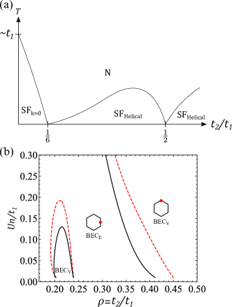
Before turning to a detailed analysis, we summarize the key results of this work. We study a Bose-Hubbard model with frustrated nearest-neighbor (NN) and next-nearest-neighbor (NNN) hoppings, and . For intermediate frustration , its band structure features a closed contour minimum centered around the point (). We then consider a bosonic condensate with a macroscopic wavefunction at a single momentum on the contour minimum – a “helical condensate”, where is the condensate density, and are the phase and density fluctuations, respectively. As illustrated in Fig. 1, the helical superfluid is a stable phase on the high symmetry points of the contour with its transition temperature to the normal state (below that of a conventional superfluid in the unfrustrated regime ) strongly suppressed by quantum and thermal fluctuations. Quantum Lifshitz transitions at 111The quantum Lifshitz transition at only happens at the vertices of the hexagonal contour (see Fig. 5), which is energetically stable at one-loop order as shown in Fig. 1(b). Higher-order fluctuations may shift the positions of the Lifshitz transitions, or make the transition at split into two Lifshitz points characterized by smectic-like Goldstone modes with Lagrangian (44b), as allowed by the lattice symmetry. are characterized by “soft” Goldstone modes that exhibit an anisotropic quartic dispersion, which suppresses the transition temperature to zero.
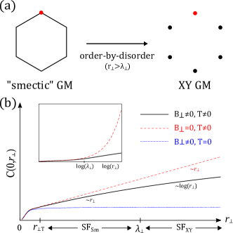
As summarized in Fig. 2, at zero temperature () and on scale shorter than quantum order-by-disorder length , the highly anisotropic superfluid exhibits an unconventional smectic-like Goldstone mode (GM) with a low-energy dispersion [for full dispersion, see Eq. (31)]
| (1) |
where the subscript () denotes the direction that is parallel (perpendicular) to condensate momentum , located at the high symmetry points of the dispersion contour. At temperatures higher than the interaction , the crossover scale is modified to . On longer scales the so-called order-by-disorder sets in, driven by quantum, thermal and lattice effects, and the system crossovers to a more conventional superfluid with highly anisotropic linear dispersion. In the weakly-interacting limit, the order-by-disorder length is long, given by
| (4) |
To further explain the order-by-disorder phenomenology (discussed in detail in Sec. V), we first note that the thermodynamic potential of the helical state near the condensate momentum [see the right panel of Fig. 2(a)] exhibits a property
| (5) |
where the coefficients and are dominated by the bare dispersion (see Appendix B), while is generated perturbatively by the lattice order-by-disorder via interaction . In the above, is the condensate number. The corresponding low-energy Goldstone mode Lagrangian density is given by
| (6) |
which when treated at a quantum level leads to the dispersion (1) for ( the lattice constant). We observe that a difference choice of the helical condensation, , equivalently corresponds to a linear in phase rotation, . By applying the two transformations to the thermodynamic potential and the Goldstone mode Hamiltonian respectively, and requiring the shifted energies to be identical, we obtain the following Ward identities,
| (7) |
We expect the relations (7) to hold at all order of a perturbation theory (see Sec. V). In particular, at the zeroth order, the thermodynamic potential [see the left panel of Fig. 2(a)] is featured by a degenerate contour minimum, and thus . At one-loop (first) order, the correction to the thermodynamic potential is given by the zero-point energy of the Bogoliubov quasiparticles together with entropic contributions, which in turn gives a () for () in the weakly-interacting limit. We also perform a complementary calculation of verifying (7). In contrast, while at zeroth-order, the above symmetry does not constrain it to hold generically.
The Goldstone mode theory (6) predicts the low-energy properties of the helical superfluid. In particular, the off-diagonal order of the superfluid , where . As shown in Fig. 2(b), the two-point correlation function exhibits several qualitatively distinct limits. Here we focus on the behavior along the direction, leaving detailed discussions in Sec. IV.1. At zero temperature (see the blue-dotted curve), for either or , , indicating a long-range order of the helical superfluid. At nonzero temperature, as illustrated by the black (red-dashed) curve, () for (), which signifies a quasi-long-range (short-range) order as a consequence of the XY (smectic) GM fluctuations. For a general case and , there are two important crossover scales, and . The former separates the low-temperature quantum and higher-temperature classical regimes, while the latter, as discussed above, separates the short-distance smectic and long-distance XY regimes.
| Observables | 2d Helical SF | 2d conventional SF |
| Static structure factor, | ||
| Condensate depletion, | ||
| Momentum distribution, | , when , when | , when , when |
|---|---|---|
| Superfluid stiffness, | ||
| Chemical potential correction, | logarithmic correction Popov (1972); Salasnich and Toigo (2016) |
Consequently, the helical state is characterized by an anisotropic XY superfluidity at the longest scale. However, within a large (for small ) order-by-disorder crossover scale, ( the coherence length), the system exhibits soft () quantum and thermal fluctuations, with its physical properties qualitatively distinct from that of a conventional superfluid. Abstracting from the Bose-Hubbard lattice model, we develop a field theory that captures the key qualitative features of the helical superfluid within this regime, and calculate a number of its physical observables, with the zero-temperature results summarized in Table 1. At nonzero temperature, thermal fluctuations set in at scales beyond (), as illustrated in Fig. 2(b). Such quantum-to-classical crossover is observable in real space- or momentum-resolved quantities, as exemplified by the structure factor in Sec. IV.2.1. We now turn to detailed analysis that leads to the results enumerated above.
III Frustrated Bose-Hubbard model on honeycomb lattice
To explore the phenomenon of nonzero momentum helical superfluidity, we study a frustrated Bose-Hubbard model on honeycomb lattice with Hamiltonian , where
| (8) |
is the usual on-site interactions with the subscripts and labeling the Bravais lattice sites and the two sublattices respectively. is the boson number operator with and the corresponding creation and annihilation operators. The kinetic part of the Hamiltonian is given by
| (9) |
where and are the nearest-neighbor (NN) and the next-nearest-neighbor (NNN) hopping parameters, respectively. We focus on the case of , taking the advantage of the symmetry of the model: , . In contrast to the NN hopping, we take the NNN hopping, , to be “frustrated antiferromagnetic”, . This has been engineered in atomic systems in an optical lattice through Floquet techniques Wintersperger et al. (2020). Throughout our analysis below, we use dimensionless parameter to quantify the frustration in this model.
III.1 Band structure of non-interacting Hamiltonian
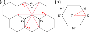
Below we first review the band structure of , identifying the condition when a degenerate minimum along a closed contour develops, and then study a Bose condensate on the this dispersion minimum contour via Bogoliubov approximation. We start with specifying the NN and NNN vectors as [see Fig. 3(a)]
| (10) |
with the lattice vectors spanning the Bravais triangular lattice and the unit vectors spanning the honeycomb lattice (the lattice constant ). The corresponding reciprocal vectors are [see Fig. 3(b)]
| (11) |
The Hamiltonian (9) is straightforwardly diagonalized in momentum space (see Appendix A)
| (12) |
where
| (13) |
create bosonic excitations in the two bands,
| (14) |
exhibiting Dirac nodes at the points (the corners of the first Brillouin zone), made famous in graphene but irrelevant here for bosonic system dominated by condensation at the bottom of the band. In the above,
| (15) |
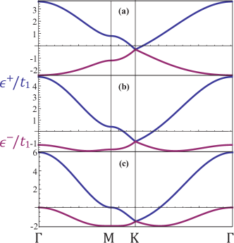
with . The dependence of the band structure on is depicted in Fig. 4.
Momenta is the dispersion minimum that satisfies
| (16) |
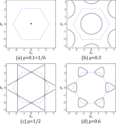
As shown in Fig. 5, controls the form of the dispersion minimum in the reciprocal space. In detail, for , the minimum is at the point (), while for , the minima are located at the points. For intermediate frustration (), the dispersion minima are extended to closed contour(s) centered around the (K) point(s). This macroscopic degeneracy makes the system sensitive to perturbations. Below we discuss these three cases respectively.
III.1.1
The simplest is the weakly-frustrated case of , for which the bosons condense at the point [see Fig. 5(a)], exhibiting conventional zero momentum superfluidity. In the XY spin language, this corresponds to a ferromagnetic spin state.
III.1.2 Intermediate frustration,
In this case, the energy minima form closed contours encircling six corners of the first Brillouin zone, as shown in Fig. 5(d), with contours shrinking as increases to .
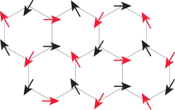
As , two sublattices decouple, with bosons on each triangular lattice condensing at a K point of the reciprocal lattice.444In XY spin language, this corresponds to the coplanar state, the ground state of XXZ model on the triangular lattice. Generally, such superfluid is described by two order parameters where are two independent complex condensate amplitudes at . Each of these site-dependent order parameters can be written as a two component XY vector . For a particular choice of , a configuration of is pictorially illustrated in Fig. 6.
III.1.3
The intermediate-frustration regime – the main focus of this paper – exhibits a closed dispersion minimum centered around the point, as illustrated in Fig. 5(b). Generically, the contour exhibits a lattice symmetry. The contour degenerates into a circle [hexagon] for , see Fig. 5(b) [, see Fig. 5(c)].
III.2 Helical superfliud in Bogoliubov approximation
The interplay of interactions and the macroscopic degeneracy discussed above presents a rich and challenging problem. However, for weak interactions, a Bose condensate on a finite set of points555This is to be contrasted with an exotic Bose-Luttinger liquid state, where the boson amplitude is ordered with fluctuating across the entire contour, as recently studied by Sur and Yang Sur and Yang (2019) and Lake et al. Lake et al. (2021) on the minimum of the dispersion contour is at least a locally stable state of matter. For a set of non-collinear points, the ground state is a supersolid that generically breaking the underlying crystal lattice and the U(1) symmetries. A simpler collinear superfluid states are represented by a helical FF-like condensate at a and an LO-like condensate at Radzihovsky (2011); Choi and Radzihovsky (2011). For interacting bosons, finding a ground state even among these set of supersolids (characterized by a set of ) is a challenging problem that we do not address here and is best studied numerically.
Here we focus on a helical superfluid corresponding to a condensation at a single that we find exhibits rich phenomenology that we explore in detail. Such a state can also be described by a helical spin density wave that breaks the lattice rotational and time-reversal symmetries. However, in this FF helical state, the physical observables remain (lattice-) translationally invariant.
Thus, focusing on such a helical condensate at , we study interacting bosons on a frustrated honeycomb lattice (9) within the Bogoliubov approximation in a canonical ensemble. In momentum space, the interaction (8) is given by
| (17) |
where is the number of the unit cells, which is one-half of the number of the sites, . At low energies, neglecting inter-band excitations, we can focus on the lowest band, and express the site boson operators and in terms of the lower-band operator ,
| (18) |
where defined in Eq. (15). Expressing the Hamiltonian in terms of excitations
| (19) |
out of a helical condensate , to quadratic order we have the Bogoliubov Hamiltonian,
| (20) | ||||
| (24) |
where
| (27) |
and
| (28) |
deferring details to Appendix C. Bogoliubov-diagonalizing the Hamiltonian gives
| (29) |
where the ground state energy
| (30) |
and the dispersion
| (31) |
with
| (32) |
and
| (33) |
We postpone the discussion of until Sec. V, where we show that fluctuations together with the lattice effects lead to order-by-disorder selection of the condensation at high symmetry points of the contour. In anticipation of this, here we note that there are two classes (and equivalents) of high symmetry points represented by “Vertex” and “Edge” , with (16) giving,
| (34) |
We next examine the details of the Bogoliubov dispersion that is positive-semi-definite (gapless at ) for all and , which for reduces to . We thus find that the helical condensate at the Bogoliubov level is locally stable.
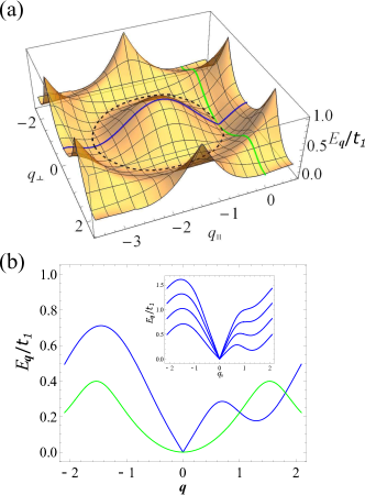
In Fig. 7, we plot the quasiparticle dispersion as a function of , where and . Without loss of generality, we plot the case , which illustrates general properties of the dispersion (31). We note that it is asymmetric under due to the contribution in (33). Physically, this broken inversion symmetry is a consequence of the spontaneously-chosen . At , the disperion also displays a metastable saddle point inherited from the contour minimum in the noninteracting dispersion , as shown by the blue curve in Fig. 7(b). This feature disappears gradually with increasing interaction [see inset of Fig. 7(b)]. In the small limit, as expected on rotational symmetry grounds (here neglecting lattice order-by-disorder effects, but see Sec. V) of a helical superfluid (striped) state, the dispersion is well-described by an anisotropic smectic form,
| (37) |
with a “soft” direction [see the green curve in Fig. 7(b)], where . For , the and can be neglected at small , while in the rotational invariant limit , . The parameters in Eq. (III.2) can be obtained by expanding the free dispersion in with the results given in Appendix B. We note that at the Lifshitz transition, . Then, the (above neglected) higher-order contribution should be taken into account, with the Goldstone mode exhibiting an anisotropic quartic dispersion in all directions.
IV field theory of helical superfluid on a closed contour minimum
We now turn to a complementary continuum field-theoretic description of the helical superfuild state, characterized by Bose condensation on a closed contour minimum in momentum space. In the isotropic case, neglecting lattice effects, this physics can be encoded through a quartic dispersion
| (38) |
with minima on a contour . As we demonstrated in Sec. III, such dispersion is indeed realized for bosons on a honeycomb lattice for , with
| (39) |
We can encode this physics in a noninteracting Hamiltonian with
| (40) |
We then extend this to an interacting field theory and study it in a grand canonical ensemble, with the corresponding imaginary-time action ,
| (41) |
a complex bosonic field and the chemical potential. We also defined an energy offset and interaction parameter inherited from the Hubbard model.
As with the lattice model in Sec. III, here we focus on the helical superfluid state – a condensate at a single point on the dispersion contour minimum – encoded in , (38), and in (41). In the density-phase representation, the state is characterized by
| (42) |
with a nonzero condensate density (at mean-field level) and momentum , for (vanishing otherwise), and density and phase fluctuations, and , respectively. To quadratic order, the helical superfluid is then described by a Goldstone mode Lagrangian density 666 Each term in Eq. (41) can be rewritten in terms of and as
| (43) |
where the subscripts and denote axes parallel and perpendicular to , respectively. In Sec. V, we will consider higher-order fluctuations that renormalize the parameters , and reduce the symmetry of the Lagrangian by lattice effects. We note that the phase is compact with periodicity, and thereby allows vortex configurations – dislocation in the helical pattern of the state. However, because we are primarily interested in the ordered helical superfluid at zero temperature, where these defects are confined, we will neglect them in most of our analysis. They are however important for the finite temperature Kosterlitz-Thouless superfluid-to-normal transition in Fig. 1(a).
Integrating out field in Eq. (43), we obtain the effective theory of described by a quantum smectic Lagrangian (consistent with the honeycomb lattice model analysis in Sec. III)
| (44a) | ||||
| (44b) | ||||
where Fourier transform of the operators and are given by
| (45) |
with the couplings777At and weak interaction, we neglect the difference between the boson and condensate densities, and , with , see Eq. (83).
| (46) |
The final form in Eq. (44b) corresponds to the asymptotic long wavelength limit. The superfluid mode exhibits an unusual dispersion given by
| (49) |
consistent with our lattice analysis, Eq. (31) and the features illustrated in Fig. 7. Two length scales emerge from the zero-sound dispersion (49). The crossover scale is the coherence length along , beyond which the dispersion is controlled by interaction. The length characterizes the anisotropy along () and transverse () to . The corresponding momentum separates the noninteracting regime, , for from the long-wavelength interacting form, , for . The latter agrees with the predictions of the lattice model, Eq. (III.2), if the lattice symmetry breaking effects are neglected.
Importantly, we note that, in the absent of lattice effects, is absent in the expansion of Eq. (44b) at all orders. This is enforced by the underlying rotational symmetry that is spontaneously broken by the helical superfluid state. More explicitly, an infinitesimal shift of the condensate momentum along the dispersion minimum contour is a symmetry888This is closely related to the spontaneous breaking of dipole conservation (in addition to charge) of Bose condensation, which prohibits linear derivative terms, as recently studied in the dipolar Bose-Hubbard model by Lake et al. Lake et al. (2022) Here, the helical superfluid is characterized by an emerged dipole conservation perpendicular to , which however, only holds infinitesimally.. According to (42), this transforms , which then enforces the exact vanishing of the coefficient of .
IV.1 Stability
We now turn to the analysis of the stability of the helical condensate at to quantum and thermal fluctuations, characterized by Goldstone mode fluctuations, . The divergence of this fluctuations in the thermodynamic limit is a signature of instability. We generalize our analysis to space-time dimensions, with two “hard” axes, and , and transverse “soft” axes. A complementary generalization to “columnar” Goldstone mode (with “hard” and “soft” axes) is relegated to Appendix D. At , both generalizations reduce to the physical case of interest, but corresponding to distinct analytical continuation of the physical problem. Below, we employ the low-energy Goldstone mode theory, (44b), valid within a UV cutoff defined by .
IV.1.1 Local fluctuations
At zero temperature, quantum fluctuations are quantified by
| (50) |
and is finite (system size independent) in the thermodynamic limit. This thereby demonstrates the stability of the helical condensate to quantum fluctuations.
At nonzero temperature, thermal fluctuations are dominated by the zeroth Matsubara frequency , where , with . This gives
| (54) |
where the dimensionless parameters and . and are the system size along the and directions, respectively. We thus observe that for , (in a striking contrast to a conventional superfluid) thermal fluctuations diverge with system size, and thereby destabilize the helical condensate at any nonzero temperature in the thermodynamic limit. For the physical case of , the length scales for this instability are set by .
IV.1.2 Two-point correlation function of
Next, we calculate the static two-point correlation function of , in the physical case given by
| (55) |
We are interested in its asymptotics in the high-temperature classical and low-temperature quantum limits. At , the Matsubara converts into an integral over a continuous frequency , giving
| (56) |
growing quadratically to a finite asymptote , (50), at .
In the high-temperature limit, only contributes to the correlation function, giving
| (59) |
where is the error function Toner and Nelson (1981); Radzihovsky (2011).
The above analysis indicates a crossover between the low and high temperature limits of . To this end, we perform Matsubara summation in Eq. (55) using
| (60) |
and define a crossover scale
| (61) |
separating the quantum () and classical () regions of momenta. This gives
| (62) |
where . At low temperature, and , the quantum, second term dominates, giving . While at high temperature, and , is dominated by the classical, first term, giving .
IV.1.3 Order-by-disorder
Although the effective theory introduced in this section is unstable to thermal fluctuations for , we anticipate that the presence of the underlying honeycomb lattice explicitly breaks the degenerate contour in Eq. (40) down to six-fold minima through quantum and thermal fluctuations, that probe all momentum scales (detailed in Sec. V). This in turn introduces perpendicular stiffness , modifying the low-energy Lagrangian to
| (64) |
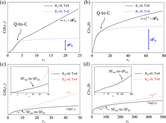
with suppressed fluctuations. As discussed in Sec. V, () for () in the weakly-interacting limit . Importantly, this leads to a crossover length scale . Consequently, as illustrated in Fig. 8(c)(d), the helical superfluid exhibits an extended crossover from a smectic regime to an anisotropic XY regime (but with the condensate at finite momentum), separated by . Since is perturbatively small in , can be very large, exhibiting long range of anomalous smectic superfluidity, that we study in detail below.
IV.2 Physical observables in smectic superfluid regime
IV.2.1 Structure factor
To calculate the structure factor, we employ the Lagrangian (43). In Fourier space, it is given by
| (65) |
where
| (68) |
with and defined in Eq. (45).
The structure factor is the density-density correlation function, in the Fourier space given by
| (69) |
This static structure factor is then given by
| (70) |
where is defined in Eq. (49) and we used Eq. (60) to carry out the Matsubara sum.
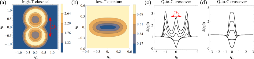
The structure factor (70) depends on the a number of scales: coherence length , anisotropic length factor and parallel thermal wavevector . Below we first present the results in the low- and high-temperature limits, and then discuss the crossover between them.
In the high-temperature limit, , the structure factor becomes
| (73) |
exhibiting a maximum on a closed contour (inherited from the noninteracting dispersion minimum) with a height and a width increasing with , illustrated at high temperature in Fig. 9(a).
In the complementary low-temperature limit, , the structure factor becomes
| (76) |
in contrast exhibiting a single minimum at , which becomes more shallow with increases , as shown in Fig. 9(b). It can be written as a scaling form
| (77) |
in the limits, and , with
| (78) |
IV.2.2 Condensate depletion
The condensate depletion is given by
| (79) |
where is an infinitesimal positive number to encode operator time ordering and with in Eq. (42) expanded up to quadratic order in and ,
| (80) |
with matrix given in Eq. (68), given in Eq. (49) and
| (81) |
After performing the Matsubara summation in Eq. (79) and using the identity (60),
| (82) |
where the first term gives the zero-temperature interaction driven depletion while the second term describes additional depletion due to thermal excitations.
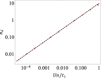
At zero temperature, the depletion (with details relegated to Appendix E) is given by
| (83) |
where with and .
At nonzero temperature, the depletion in Eq. (82) diverges in the thermodynamic limit for , as analyzed in Appendix E, indicating helical superfluid thermal instability as found in Sec. IV.1.1.
For the microscopic lattice model discussed in Sec. III, the depleting is still given by (82), but with and given by
| (84) | ||||
where the lattice effects are encoded in the periodic (in momentum space) forms of and defined in Eqs. (28) and (33).
At zero temperature, the depletion as a function of is computed numerically and presented in Fig. 10. At small , it is a power-law as found in Eq. (83). As increases, deviates from this perfect power-law given by a weakly interacting field theory. At nonzero temperature, thermal fluctuations still destroy the condensate, as discussed above.
IV.2.3 Momentum distribution
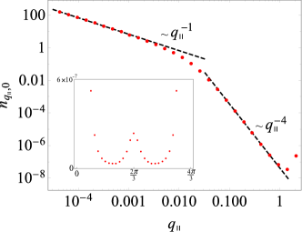
Another important characterization of the helical superfluid is the momentum distribution, . At , it is given by
| (85) |
The behavior of below () and beyond () the coherence length is described by the following scaling form,
| (86) |
with the anisotropy length scale given by and
| (87) |
We note that for , . In the opposite limit, , the momentum distribution is asymptotically given by
| (90) |
This contrasts qualitatively with that of a conventional superfluid (see Table 1).
Lattice effects beyond this field theoretical treatment are straightforwardly incorporated with at , with the lattice form of given by Eq. (84). In Fig. 11, we plot as a function of which verifies the scaling behavior () for (). Note, somewhat surprisingly the () momentum distribution is symmetric under the inversion of momentum , and its profile has the reflection symmetry, e.g. with respect to , due to the underlying lattice structure, as shown in the inset of Fig. 11. As a result, the tail is only visible for sufficiently small .
IV.2.4 Superflow
As in a conventional superfluid a spatial gradient of gives rise to a supercurrent,
| (91) |
characterized by the anisotropic superfluid velocity with its form obtained from the Noether’s theorem or, equivalently by gauging (see Appendix F)
| (92) |
We emphasize that in of (92) we included higher-order terms, previously left out in the quadratic Lagrangian, (43). For the simplest uniform gradient configuration , we have
| (93) |
with
| (94) |
In the long-wavelength limit to linear order, the supercurrent is given by
| (95) |
with the superfluid stiffness , which vanishes transversely to . This helical condensate thus (in the absent of stabilizing lattice effects) cannot maintain a superflow perpendicular to , and thus by this criterion is not a superfluid.
IV.2.5 Chemical potential
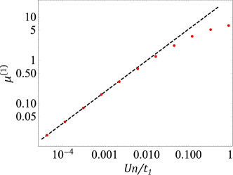
We next calculate the equation of state, given by the chemical potential as a function of the boson density ,
| (96) |
where ground state energy is given by Eq. (30). The lowest-order mean-field contribution and the one-loop correction are respectively given by
| (97) |
where in the last line we neglected lattice effects and took .
Performing the integration (see Appendix G), we obtain
| (98) |
where constants , and . The dimensionless factor in expressed in terms of microscopic parameters is given by
| (99) |
where is given by Eq. (39) in the limit of . For a general dimensional helical superfluid, this dimensionless factor is given by
| (100) |
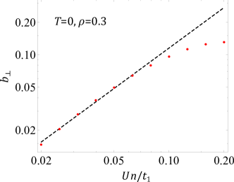
In Fig. 12, we plot an exact numerical evaluation of the chemical potential in Eq. (IV.2.5) with lattice effects as a function of . At small , Eq. (98) fits the data well. We note, as indicated in Eq. (98), decreases (increases) if () increases, in qualitative distinction from a conventional superfluid (see Table 1).
V Order-by-disorder
So far, we studied the helical condensation at a single momentum on the dispersion minimum contour at the Bogoliubov level. At this order, it exhibits smectic fluctuations that are qualitatively larger than that of conventional XY superfluids due to the macroscopic degenerate ground states. In this section, we go beyond the quadratic action, and study the order-by-disorder phenomenon that appears due to the interplay of quantum and thermal fluctuations, and the lattice effects. This generates a nonzero that stabilizes the helical superfluid even at nonzero temperature.
Formally, we work with the coherent state path integral of the lattice model introduced in Sec. III, where the partition function is given by , with the imaginary-time action and the corresponding Lagrangian
| (101) |
In the above, and are functionals that respectively have the same expressions as the kinetic and the interacting parts of the Hamiltonian introduced in Sec. III with the operators and replaced by coherent state fields and . To study the helical superfluid, we consider the density-phase fluctuations around a mean-field of a helical condensate with density and momentum :
| (102) |
where is the position of the lattice site in sublattice. Below, we drop the subscripts and for notation simplicity. Then, the action can be written as with the constant mean-field part (zeroth-order thermodynamic potential) and the bare Lagrangian, . Such a procedure parallels the field theoretical approach in Sec. IV, but now encodes the underlying lattice effects. Analysis of the quadratic part of the action reproduces the Bogoliubov results, predicted in Sec. III. To study the effects of the higher-order nonlinearalities, various approximation schemes can be employed. Here we safely employ an analysis perturbative in , self-consistently verifying the corrections to are finite. We thereby formally obtain
| (103) |
where the renormalized thermodynamic potential and Lagrangian are given by perturbation series and [“” stands for the nth loop correction], respectively. Similar to a conventional superfluid, global U(1) symmetry ensures that is massless, i.e., in the continuum, only gradients of appears in the Lagrangian. For a helical condensate, another constraint is the equivalence of the transformations and in the long wavelength limit. The former transforms the free energy,
| (104) |
The latter, when applied to the continuum Lagrangian density (discussed in detail in Appendix H),
| (105) |
gives an energy shift . In the above, the ellipsis denotes and higher derivative terms. Since can be chosen arbitrarily, we conclude that
| (106) |
for any integers , holding in every nth order of the perturbation theory, . Below, we study the order-by-disorder phenomenon by performing one-loop calculations of and for both zero and nonzero temperatures.
V.1 Thermodynamic potential
Before working in the more convenient functional integral formalism, we note the ground state energy in Eq. (30) consists of two contributions, the mean-field and the zero-point energies, respectively, given by
| (107) |
The former is the dominate contribution that exhibits a sub-extensive degeneracy on the contour minimum, while the latter is the lowest-order in correction, corresponding to the one-loop correction in the field theory treatment below.
In the coherent-state path integral, the zeroth-order thermodynamic potential is equal to the mean-field ground state energy above (with )
| (108) |
and the one-loop correction (neglecting the upper band, valid for ) is given by
| (109) |
where is defined in Eq. (210). In the low-temperature limit , reduces to the zero-point energy of the Bogoliubov quasiparticles (where we measured related to the zero-point energy of the normal state). In the above, the Matsubara sum was carried out by using
| (110) |
obtained by integrating (60) over or by Poisson summation formula followed by a contour integral Altland and Simons (2010).
The perturbation theory also gives order-by-order corrections to the condensate momentum, . This allows us to study the corrections of the thermodynamic potential and its curvature as an expansion at the mean-field minimum: and .999However, the full expression is not real for any since the quasiparticle is only guaranteed to be stable when expanding the condensate around the contour minimum . This is an artifact of the perturbation theory arising from , and can be avoided in a self-consistent or renormalization group analysis. Numerical evaluation of the integral (V.1) lifts the degeneracy of the bare dispersion contour, replacing it by six minima with the lattice symmetry. We refer to this as order-by-disorder phenomenon (demonstrated in the context of frustrated magnetism in Bergman et al. (2007); Mulder et al. (2010)). As shown in Fig. 1(b), the helical condensate is stable on the high symmetry points of the contour, the Vertex () and the Edge () condensates, depending on the microscopic parameters , , and temperature . The phase boundaries are all first-order. We note that there is a reentrant around , related to the detailed quasiparticle dispersion at small characterized by and . As detailed in Appendix I, an expansion at the minimum of the thermodynamic potential gives
| (111) |
for small , which gives an effective cutoff such that . In the above,
| (112) |
with a dimensionless constant and the scaling function
| (115) |
With increasing , higher powers terms in are important, leading to a deviation from the scaling form (111), see Fig. 13.
As a consequence of the order-by-disorder phenomenon, is induced given by as discussed above. As a complementary analysis, below we perform a direct calculation of , and show that it reduces to zero in the isotropic, continuum limit.
V.2
To obtain , one first needs to calculate the zeroth-order action based on the lattice model in Sec. III. A shortcut to this is to expand the mean-field ground state energy in , and use the relation . However, this has a shortcoming as it only gives the leading order in couplings. Alternatively, one can start with the lattice model, do an expansion in and , and then take the continuum limit. The latter approach is more laborious, but gives the full expression that is valid even at large momenta. We relegate the details of this analysis to Appendix H. For simplicity, we consider a long-wavelength form in analogy to (44b) that is valid within the coherence length in the weakly-interacting limit. By including up to quartic in terms required for one-loop calculations, and choosing at one of the symmetric points, the zeroth-order Lagrangian takes the following form (with the superscripts dropped for the simplicity of notation)
| (116) |
where and , vanishing at . All the other parameters are of the form with a dimensionless constant while the explicit expressions can be obtained via along with , and , where the latter relations are found by inspecting the explicit form of the quadratic action, (207), and are given in Eqs. (B) and (B) for and , respectively. The linear derivative term (tadpole diagram) can be eliminated by choosing the condensate momentum such that , which at mean-field level, gives . We note in the Lagrangian (V.2) even in the presence of lattice (but excluding the zero-point energy) effects. This is consistent with the mean-field ground state energy in Eq. (107) that exhibits a degenerate contour minimum. However, higher-order fluctuations generally generate a nonzero . At one-loop order and the weakly-interacting limit, it is given by (see details in Appendix J)
| (117) |
where the dimensionless scaling function has the same limits as in Eq. (115) and with a dimensionless constant. In the isotropic limit , and , resulting in . This suggests the robustness of the Lifshitz transition point at at one-loop order and associated relation between harmonic and nonlinear terms enforced by the rotational symmetry of , also corresponding to the dipole conservation symmetry.
VI Conclusion
In summary, we studied a nonzero-momentum superfluid state as a condensate in a frustrated honeycomb Bose-Hubbard model that features a dispersion minimum contour with a nonzero momentum scale , set by frustrated hopping. We supplemented the lattice model by a continuum smectic field theory and explored in detail the rich phenomenology that emerges from the helical (single momentum) Bose-condensation on this dispersion minimum contour.
Consistent with generalized Hohenberg-Mermin-Wagner theorem Mermin and Wagner (1966); Hohenberg (1967); Halperin (2019), we found that the helical condensate is stable at zero temperature despite quantum fluctuations that are qualitatively stronger than that of a conventional superfluid. The helical state is spontaneously highly anisotropic in its spectrum of low-energy excitations. We explored in detail the physical properties of such state, such as the equation of state (chemical potential), condensate depletion, momentum distribution, structure factor, of all which are qualitatively distinct from a conventional XY zero-momentum superfluid. Because of the “soft” smectic dispersion, at nonzero temperature, thermal fluctuations that diverge in the absence of lattice effects lead to a vanishing of the helical condensate.
However, somewhat paradoxically, a subtle interplay of lattice effects with quantum and thermal fluctuations leads to stabilization of the helical smectic state, through the phenomenon of order-by-disorder via a crossover to a more conventional stable XY superfluid.
Our study thus predicts a stable helical superfluid state and its rich phenomenology that can emerge in frustrated bosonic systems, characterized by a bare dispersion minimum contour. Such sub-extensive contour degeneracy of the condensate momentum, , can be realized in cold atom experiments through Floquet engineering of the optical lattice with frustrated hopping Struck et al. (2011); Wintersperger et al. (2020) or synthetic Rashba spin-orbit coupling Zhai (2015). Because the latter approach is not based on frustration, its closed contour minimum dispersion would be spoiled by an optical lattice, reduced to a discrete set of dispersion minima Zhang et al. (2013); Toniolo and Linder (2014); Mæland et al. (2020). It would thereby exhibit a bare modulus controlled by the depth of the optical lattice, rather than Feshbach tunable interactions Chin et al. (2010), as considered in our study. Yet, in a shallow optical lattice with a weak , within a long crossover scale we expect a nonzero momentum condensate Wu et al. (2011); Barnett et al. (2012); Cui and Zhou (2013) in spin-orbit coupled Bose gases, exhibiting phenomenology predicted in Table 1.
The frustrated bosonic model that we studied is isomorphic to a quantum O(2) easy-plane magnet with frustrated exchange couplings, which is also characterized by a spiral contour as manifold of its classical ground states. The helical superfluid we explored thus maps directly on such a coplanar spin spiral state with the U(1) superfluid phase corresponding to the O(2) direction of the XY spin. Theoretical studies suggest the stability of such spiral states in a quantum easy-plane magnet Liu et al. (2020) and in XY models (for spin-1/2, equivalent to the Bose-Hubbard model at half-filling in the hard-core limit, in contrast to the weak limit considered here) with at high symmetry points selected by quantum fluctuations (Varney et al., 2011; Di Ciolo et al., 2014; Sedrakyan et al., 2015). This contrasts with the corresponding Heisenberg O(3) model Bergman et al. (2007); Mulder et al. (2010), which at nonzero temperature in 2d is always unstable (even with the usual linear dispersion) to a disordered state due to strongly coupled nonlinear spin wave fluctuations.
Our analysis, however, does not provide the sufficient conditions to realize the helical superfluid discussed here. Other interesting supersolid phases, e.g., Bose condensate at multiple momenta, are also competing ground states that can emerge from the interplay of interactions and the macroscopic degeneracy of the dispersion minimum. Selecting between these is a challenging problem that we have not addressed and likely requires extensive numerical analysis. Cold-atoms systems where our model is realized using Floquet engineering will likely be challenged by heating problem as well as further neighbor hopping and interactions.
Here we neglected the vortices (allowed by the periodicity of the superfluid phase) that can play an important role for the quantum and thermal phase transitions out of the helical superfluid state, sketched at the mean-field level in Fig. 1(a). In 2+1d it is isomorphic to the melting of a quantum smectic (at low energies perturbed by stabilizing modulus generated by order-by-disorder) that has been formulated through a dual gauge theory in Ref. Radzihovsky (2020); Zhai and Radzihovsky (2021), but with critical RG analysis remaining as an open problem. We note that, as discussed in Ref. Yan and Reuther (2022) in addition to conventional vortices of the superfluid phase , thermal excitations of orientational (“momentum”) vortices in (based on numerical analysis) appear to play an important role. We leave these and other questions discussed above for future theoretical research and hope that the rich phenomenology presented here will stimulate further experimental and theoretical works on frustrated bosonic and magnetic systems.
Acknowledgement
L. R. thanks Arun Paramekanti for discussions. This work is supported by the Simons Investigator Award to L. R. from the James Simons Foundation. L. R. also thanks the KITP for its hospitality as part of the Spring 2022 Pair-Density-Wave Order Rapid Response Workshop, during which part of this work was completed and in part supported by the National Science Foundation under Grant No. NSF PHY-1748958. Research at Perimeter Institute is supported in part by the Government of Canada through the Department of Innovation, Science and Economic Development Canada and by the Province of Ontario through the Ministry of Colleges and Universities.
Appendix A Diagonalization of frustrated tight-binding model on honeycomb lattice
The tight-binding Hamiltonian in Eq. (9) can be written in terms of Pauli matrices , where
| (118) |
with
| (119) |
The Hamiltonian can be diagonalized by the transformation
| (120) |
which gives
| (121) |
with two bands
| (122) |
The lower band exhibits a contour minimum for .
In general, the dispersion minimum contour can appear in a class of Hamiltonians written as
| (123) |
where and are the nearest-neighbor and next-nearest-neighbor hopping amplitudes and is a hopping matrix, with the form
| (124) |
in the sublattice basis. Then the two band are given by
| (125) |
with the lower energy band exhibiting macroscopic ground state degeneracy along the contour defined by .
Appendix B Expansion of around the dispersion minimum contour
In the weakly-interacting regime, the band dispersion around the bose condensate plays an important role for the low-energy properties of the helical superfluid. This is established through the facts: (i) the zeroth-order thermodynamic potential depending on the free dispersion and (ii) The relation between and the zeroth-order Goldstone mode theory as discussed in Sec. V. Expansion on the lower band dispersion (14) up to quartic order gives
| (126) |
where for the Vertex condensate (), , , and the coefficients
| (127) |
and for the Edge condensate (), , , and the coefficients
| (128) |
In the above, , which vanishes at . For , there are corrections to all the coefficients above, but here we only give the ones for and that are important for the one-loop calculations in Sec. V.
Appendix C Bogoliubov approximation to the frustrated Bose-Hubbard model
For a condensate at , the bosonic operators are given by
| (129) |
where and . We then expand the interacting part of the Hamiltonian, (17), which up to quadratic order of and is given by
| (130) |
With a transformation to the band basis
| (131) |
followed by neglecting the upper band contributions, , that only give corrections to the ground state, we obtain the following total Hamiltonian
| (132) |
which gives the Hamiltonian (24) after using the canonical ensemble relation
| (133) |
The Hamiltonian (24) then can be diagonalized by the bosonic Bogoliubov transformation
| (134) |
where and (chosen to be real) are given in Eq. (84) with , and is a nonunitary matrix that preserves the bosonic commutation relation after the basis transformation
| (135) |
The dispersions of in Eq. (31) can be obtained by solving the determinant equation
| (136) |
with the solutions , , where .
Appendix D Stability of quantum “smectic” and “columnar” phases in d-dimensions: generalized Hohenberg-Mermin-Wagner theorems
In this appendix, we perform a simple dimensional analysis of the stability of a smectic (columnar) phase in spatial dimensions, which exhibits a Goldstone mode with () hard direction(s), , and the other () soft direction(s), . We set for simplicity.
For the smectic phase, the quantum fluctuations at is characterized by
| (137) |
With the change of variables , the above equation becomes
| (138) | ||||
The stability of this state requires the convergence in the IR, which requires
| (139) |
For the columnar phase, the quantum fluctuations are
| (140) |
which requires
| (141) |
for the stability. Therefore, for the physical dimension of our interest, , both requirements are satisfied, which suggests the helical superfluid stable under quantum fluctuations.
At nonzero temperature, we consider the dominant classical contributions at , which for the smectic are given by
| (142) |
Its stability requires
| (143) |
While in the columnar phase,
| (144) |
which requires
| (145) |
Thus, thermal fluctuations make the 2d smectic/columnar phase unstable.
Appendix E Calculation details of depletion
The condensate depletion is given by Eq. (82) at weak interactions as discussed in the main text. At zero temperature, leads to
| (146) |
where as defined in Eq. (45). In this section, we perform the integral exactly. With the change of variables:
| (147) |
the integral can be rewritten as
| (148) |
where and
| (149) |
with
| (150) |
Consequently, the integral is
| (151) |
which gives the depletion
| (152) |
Similarly, we generalize the study of depletion to be in dimensions. The system possesses dispersion hard along directions and soft along directions. With being the momentum along the -th hard (soft) direction, the generalized dispersion is
| (153) |
In terms of variables
| (154) |
the depletion is given by
| (155) |
The integral can be proceeded as
| (156) | |||||
| (157) |
Particularly, when and for any and ,
| (158) |
The depletion is then given by
| (159) |
Now we discuss the thermal corrections to the depletion, which is given by
| (160) |
with and defined in Eq. (31), and and defined in Eq. (84). In the long-wavelength limit, . Then, with the change of variables and (set and for simplicity),
| (161) |
where the radial integral over is finite if . This suggests the superfluid is stable when
| (162) |
For a smectic (columnar) phase with () and (), we reproduce the stability condition () as obtained in Appendix D.
Appendix F Superflow
In this section, we derive the expression of the supercurrent. Notice that there involves higher-order derivatives in the Lagrangian in Eq. (41), its equation of motion is thus modified as
| (163) |
where and are spatial indices. With the detailed form of , We obtain
| (164) |
along with a similar equation for . In addition, the Lagrangian respects the global U(1) symmetry. Therefore, an infinitesimal transformation (and , where ) results in with being a total derivative, given by
where we applied the equation of motion in Eq. (163) to get the second equality. Then, the Noether current is
| (165) |
which satisfy the continuity equation, .
With (and at mean-field level ), the supercurrent is then a current in space,
| (166) |
generated through the twisting of the superfluid phase . In the last line, we consider the long-wavelength limit, where the fluctuation of density is small such that .
The supercurrent density can be written as , where the superfluid velocity. For a linear in classical phase variation , the superfluid velocity reduces to the derivative of the bare dispersion
| (167) |
where
| (168) |
We emphasize that the existence of the nonlinear terms in Eq. (166) makes this relation hold.
Alternatively, the supercurrent can be obtained as a response to a background probe gauge field. We first generalize the long-wavelength harmonic Goldstone mode Hamiltonian density [with the corresponding Lagrangian density (44b)],
| (169) |
to the quartic order in by requiring the rotational symmetry of , giving
| (170) |
As the system coupled with a background U(1) gauge field, the Hamiltonian density is modified as . The supercurrent density is then obtained by taking derivative with respect to the gauge field
| (171) |
which reproduces the long-wavelength expression in Eq. (166).
Appendix G Calculation details of the chemical potential
In this appendix, we evaluate the integral in Eq. (IV.2.5). As in Appendix E, we use the dimensionless variables defined in Eq. (147), and written integral as
| (172) |
where , is defined and computed in Eq. (148), and
| (173) | |||||
with is in Eq. (150). We note that and , which lead to the last approximation in Eq. (173).
As a result, the chemical potential for the helical superfluid in is
| (174) |
In general, for a dimensional system with a dispersion defined in Eq. (153), the integral in Eq. (172) can be generalized as
| (175) |
In terms of the dimensionless variables defined in Eq. (154), the integral becomes
| (176) |
For the special case and for any and , we have
| (177) |
Accordingly, in terms of the dimensionless quantity
| (178) |
the chemical potential is
| (179) |
where is a dimensionless constant fully determined by and . For a -dimensional smectic phase with and , the dimensionless quantity
| (180) |
We can check that with , , , and (, with dimensions of energy and length, respectively), is in fact dimensionless. On the other hand, in a columnar phase with and , the dimensionless quantity is given by
| (181) |
Appendix H theory with lattice effects
We start with the coherent state path integral formalism of the frustrated Bose-Hubbard model introduced in the beginning of Sec. V. In the density-phase representation (V), the Lagrangian (including the constant part) can be written as
| (182) |
where the kinetic part
| (183) |
and the interaction
| (184) |
For a bose condensate, we assume the fluctuations of and fields are small, and thereby expand in a power series, which up to quadratic order in and is given by
| (185) |
To perform one-loop calculations, we include the cubic and quartic terms of , given by
| (186) |
At this point, one can either directly take the continuum limit in the real space or go to momentum space to get an effective action. The calculation for the former is simpler but misses some contributions even at long length scale, while the later is tedious but valid for all momentum. We discuss both methods below.
H.1 Taking continuum limit in the real space
To take the continuum limit, we consider the fields and on lattice sites as slowly-varying functions of continuous spacetime coordinates compared to the lattice constant. The time coordinate is already continuous. Therefore, the difference of two operators at distinct spatial locations can be expanded as
| (187) |
where with and label the sublattices. Below we focus on the case while other cases can be derived following the same procedure. Including up to the second (first) order for the quadratic (cubic and quartic) term(s), the Hamiltonian density, defined by , is given by
| (188) |
where with satisfying Eq. (16),
| (189) |
and the constant and linear in terms are dropped. In the above, the dependence is hidden in and . By integrating over , we obtain the zeroth-order Lagrangian density, (V.2), with the parameters (H.1), however, not satisfying the relation . This inconsistency is due to the factor in Eq. (H), or more generally the two-band nature of the model, which invalids the simple continuum limit above that neglects the spatial variation between the two sublattice sites within a unit cell, as discussed in more details below.
H.2 Continuous effective theory in the momentum space
Alternatively, We can Fourier transform the Hamiltonian and followed by a change of basis defined as
| (200) |
where the subscripts label the two sublattices and denote the two bands as in the main text. The unitary matrix above is given by
| (203) |
At quadratic order, the action for the lower band is given by
| (207) |
where
| (210) |
In the above, we consider the weakly-interacting limit and can thereby drop the upper band contributions which only give corrections to the low energy physics. Before computing higher-order terms, we have two comments in order.
Firstly, we note the quadratic action reproduces the same Bogoliubov quasiparticle spectrum in Eq. (31). Technically, both the density-phase representation (V) and the Bogoliubov approximation (19) share the same classical background field, which in real space is given by with the and factors for the sites in the and sublattices respectively. The fluctuations around the condensate are given by and in Eq. (V) or in Eq. (19). An expansion of the former representation gives linear terms of and that takes the same form as the real and imaginary parts of in the latter representation, and thus both give the same form of the quadratic action. While the higher-order terms which modifies the in Eq. (207) do not have a simple relation compared with higher-order terms which corrects Eq. (24), they should describe the same physics.
Secondly, as shown above, an accurate calculation gives and identical with the ones from Bogoliubov theory in Eq. (III.2). In Appendix H.1, fields on the two sites within a unit cell are considered to be the same, i.e., . This is equivalent to approximate the transformation in Eq. (200) with , which gives . Therefore, the discrepancy between and in (H.1) and the accurate ones in Eq. (B) comes from the definition of the fields, which by inspection gives a factor of via the relation , and the difference between and . The latter can be neglected in the limit , where the difference is of higher-order in .
The calculations for the nonlinear terms are quite tedious. Especially, it is hard to simplify the expressions after the transformation in Eq. (200). Here, we employ the same approximation to derive below the cubic and quartic terms in .
| (211) |
where
| (212) |
where an expansion of and in small together with a Fourier transform back to the real space reproduce the nonlinear terms in the field theory (H.1) with the same coefficients obtained earlier (H.1).
Appendix I One-loop calculation of
Here we calculate the perpendicular curvature at one-loop order. By expanding the condensate momentum around its mean-field value and keeping the leading-order terms, we get
| (213) |
where can be determined by and
| (214) |
In the absence of interaction, and . Accordingly, the integrands in and are total derivatives, which makes and subsequently . In the presence of weak interaction, the dispersion deviates from the noninteracting form within a crossover scale . Therefore, the integrals (I) are dominated by the region . In this small limit, we obtain by using change of variables and in Eq. (I), where with a dimensionless constant and the scaling function is defined in Eq. (115).
Appendix J One-loop calculation of
A complete one-loop calculation should give the perpendicular stiffness of equals to the corresponding curvature in the thermodynamic potential, i.e., , with being calculated in Appendix I. Here, we instead perform an approximate calculation of in the long-wavelength limit, where the Lagrangian (V.2) is valid. Specifically, we consider the leading derivative terms and thereby only keep for the field, which is enabled by an -dependent UV cutoff defined by , which in the weakly-interacting limit reduces to . Although such calculation neglects the range of integration , the contribution to in this range is actually very small as seen in the calculation of in Appendix I that takes into account all momentum. Therefore, the integral of or actually self regulates at in the weakly-interacting limit.
J.1 Long-wavelength limit
We consider the low-energy -only theory (V.2), where the bare Green function is given by ()
| (215) |
where and .
We first calculate the coefficient of , which corresponds to the slope of the thermodynamic potential at along the direction. At one-loop order, it is given by
| (216) |
where the first term is the zeroth-order contribution that vanishes at and . With the one-loop correction, needs to be shifted such that the coefficient of is zero again, which assures is located at the local minimum of the loop-corrected thermodynamic potential with vanished first derivative. In the above, the tadpole diagrams are dropped as they cancel out up to all orders when choosing the correct .
Next we calculate , which at one-loop order is given by
| (217) |
where in the last line we choose at which the linear term vanished. In the above, the arguments of the coefficients are taken to be their mean-field value as the difference is of higher order. With a change of variables and , we can rewrite the expression above that in the weakly-interacting limit is given by
| (218) |
where (here is an integer, not confused with the particle density), and the UV cutoff indicates . In the last line above, we can read , where the dimensionless scaling function exhibits the same limits as in Eq. (115) and with a dimensionless constant.
J.2 Isotropic limit
In the isotropic limit or , the coefficients , and . Consequently, in the last line of Eq. (J.1) vanishes
| (219) |
where we used the following integration by part for the last term
| (220) |
References
- Moessner and Chalker (1998) R. Moessner and J. T. Chalker, Physical Review B 58, 12049 (1998).
- Balents (2010) L. Balents, Nature 464, 199 (2010).
- Ramirez et al. (1990) A. P. Ramirez, G. P. Espinosa, and A. S. Cooper, Physical Review Letters 64, 2070 (1990).
- Gaulin et al. (1992) B. D. Gaulin, J. N. Reimers, T. E. Mason, J. E. Greedan, and Z. Tun, Physical Review Letters 69, 3244 (1992).
- Ramirez (1994) A. P. Ramirez, Annual Review of Materials Science 24, 453 (1994).
- Uemura et al. (1994) Y. J. Uemura, A. Keren, K. Kojima, L. P. Le, G. M. Luke, W. D. Wu, Y. Ajiro, T. Asano, Y. Kuriyama, M. Mekata, H. Kikuchi, and K. Kakurai, Physical Review Letters 73, 3306 (1994).
- Dunsiger et al. (1996) S. R. Dunsiger, R. F. Kiefl, K. H. Chow, B. D. Gaulin, M. J. P. Gingras, J. E. Greedan, A. Keren, K. Kojima, G. M. Luke, W. A. MacFarlane, N. P. Raju, J. E. Sonier, Y. J. Uemura, and W. D. Wu, Physical Review B 54, 9019 (1996).
- Villain et al. (1980) J. Villain, R. Bidaux, J.-P. Carton, and R. Conte, Journal de Physique 41, 1263 (1980).
- Henley (1989) C. L. Henley, Physical Review Letters 62, 2056 (1989).
- Sachdev (1992) S. Sachdev, Physical Review B 45, 12377 (1992).
- Hastings (2000) M. B. Hastings, Physical Review B 63, 014413 (2000).
- Ran et al. (2007) Y. Ran, M. Hermele, P. A. Lee, and X.-G. Wen, Physical Review Letters 98, 117205 (2007).
- Hermele et al. (2008) M. Hermele, Y. Ran, P. A. Lee, and X.-G. Wen, Physical Review B 77, 224413 (2008).
- Evenbly and Vidal (2010) G. Evenbly and G. Vidal, Physical Review Letters 104, 187203 (2010).
- Yan et al. (2011) S. Yan, D. A. Huse, and S. R. White, Science 332, 1173 (2011).
- Depenbrock et al. (2012) S. Depenbrock, I. P. McCulloch, and U. Schollwck, Physical Review Letters 109, 067201 (2012).
- Jiang et al. (2012) H.-C. Jiang, Z. Wang, and L. Balents, Nature Physics 8, 902 (2012).
- Iqbal et al. (2013) Y. Iqbal, F. Becca, S. Sorella, and D. Poilblanc, Physical Review B 87, 060405(R) (2013).
- Iqbal et al. (2014) Y. Iqbal, D. Poilblanc, and F. Becca, Physical Review B 89, 020407(R) (2014).
- He et al. (2014) Y.-C. He, D. N. Sheng, and Y. Chen, Physical Review Letters 112, 137202 (2014).
- Gong et al. (2015) S.-S. Gong, W. Zhu, L. Balents, and D. N. Sheng, Physical Review B 91, 075112 (2015).
- Norman (2016) M. R. Norman, Reviews of Modern Physics 88, 041002 (2016).
- Mei et al. (2017) J.-W. Mei, J.-Y. Chen, H. He, and X.-G. Wen, Physical Review B 95, 235107 (2017).
- He et al. (2017) Y.-C. He, M. P. Zaletel, M. Oshikawa, and F. Pollmann, Physical Review X 7, 031020 (2017).
- Zhu et al. (2018) W. Zhu, X. Chen, Y.-C. He, and W. Witczak-Krempa, Science Advances 4, eaat5535 (2018).
- Bergman et al. (2007) D. Bergman, J. Alicea, E. Gull, S. Trebst, and L. Balents, Nature Physics 3, 487 (2007).
- Lee and Balents (2008) S. Lee and L. Balents, Physical Review B 78, 144417 (2008).
- Mulder et al. (2010) A. Mulder, R. Ganesh, L. Capriotti, and A. Paramekanti, Physical Review B 81, 214419 (2010).
- Matsuda et al. (2010) M. Matsuda, M. Azuma, M. Tokunaga, Y. Shimakawa, and N. Kumada, Physical Review Letters 105, 187201 (2010).
- Gao et al. (2017) S. Gao, O. Zaharko, V. Tsurkan, Y. Su, J. S. White, G. S. Tucker, B. Roessli, F. Bourdarot, R. Sibille, D. Chernyshov, T. Fennell, A. Loidl, and C. Rüegg, Nature Physics 13, 157 (2017).
- Biswas and Damle (2018) S. Biswas and K. Damle, Physical Review B 97, 115102 (2018).
- Niggemann et al. (2019) N. Niggemann, M. Hering, and J. Reuther, Journal of Physics: Condensed Matter 32, 024001 (2019).
- Shimokawa and Kawamura (2019) T. Shimokawa and H. Kawamura, Physical Review Letters 123, 057202 (2019).
- Gao et al. (2020) S. Gao, H. D. Rosales, F. A. Gómez Albarracín, V. Tsurkan, G. Kaur, T. Fennell, P. Steffens, M. Boehm, P. Čermák, A. Schneidewind, E. Ressouche, D. C. Cabra, C. Rüegg, and O. Zaharko, Nature 586, 37 (2020).
- Liu et al. (2020) J. Q. Liu, F.-Y. Li, G. Chen, and Z. Wang, Physical Review Research 2, 033260 (2020).
- Balla et al. (2019) P. Balla, Y. Iqbal, and K. Penc, Physical Review B 100, 140402(R) (2019).
- Balla et al. (2020) P. Balla, Y. Iqbal, and K. Penc, Physical Review Research 2, 043278 (2020).
- Yao et al. (2021) X.-P. Yao, J. Q. Liu, C.-J. Huang, X. Wang, and G. Chen, Frontiers of Physics 16, 53303 (2021).
- Bordelon et al. (2021) M. M. Bordelon, C. Liu, L. Posthuma, E. Kenney, M. J. Graf, N. P. Butch, A. Banerjee, S. Calder, L. Balents, and S. D. Wilson, Physical Review B 103, 014420 (2021).
- Gao et al. (2022) S. Gao, M. A. McGuire, Y. Liu, D. L. Abernathy, C. d. Cruz, M. Frontzek, M. B. Stone, and A. D. Christianson, Phys. Rev. Lett. 128, 227201 (2022).
- Varney et al. (2012) C. N. Varney, K. Sun, V. Galitski, and M. Rigol, New Journal of Physics 14, 115028 (2012).
- Sedrakyan et al. (2014) T. A. Sedrakyan, L. I. Glazman, and A. Kamenev, Physical Review B 89, 201112(R) (2014).
- Sedrakyan et al. (2012) T. A. Sedrakyan, A. Kamenev, and L. I. Glazman, Physical Review A 86, 063639 (2012).
- Wintersperger et al. (2020) K. Wintersperger, C. Braun, F. N. Ünal, A. Eckardt, M. D. Liberto, N. Goldman, I. Bloch, and M. Aidelsburger, Nature Physics 16, 1058 (2020).
- Zhai (2015) H. Zhai, Reports on Progress in Physics 78, 026001 (2015).
- Paramekanti et al. (2002) A. Paramekanti, L. Balents, and M. P. A. Fisher, Physical Review B 66, 054526 (2002).
- Tay and Motrunich (2011) T. Tay and O. I. Motrunich, Physical Review B 83, 205107 (2011).
- Sur and Yang (2019) S. Sur and K. Yang, Physical Review B 100, 024519 (2019).
- Lake et al. (2021) E. Lake, T. Senthil, and A. Vishwanath, Physical Review B 104, 014517 (2021).
- Gromov (2019) A. Gromov, Physical Review X 9, 031035 (2019).
- Radzihovsky (2020) L. Radzihovsky, Physical Review Letters 125, 267601 (2020).
- Yuan et al. (2020) J.-K. Yuan, S. A. Chen, and P. Ye, Physical Review Research 2, 023267 (2020).
- Gorantla et al. (2022) P. Gorantla, H. T. Lam, N. Seiberg, and S.-H. Shao, Phys. Rev. B 106, 045112 (2022).
- Lake et al. (2022) E. Lake, M. Hermele, and T. Senthil, Phys. Rev. B 106, 064511 (2022).
- Radzihovsky (2011) L. Radzihovsky, Physical Review A 84, 023611 (2011).
- Popov (1972) V. N. Popov, Theoretical and Mathematical Physics 11, 565 (1972).
- Salasnich and Toigo (2016) L. Salasnich and F. Toigo, Physics Reports Zero-point energy of ultracold atoms, 640, 1 (2016).
- Choi and Radzihovsky (2011) S. Choi and L. Radzihovsky, Physical Review A 84, 043612 (2011).
- Toner and Nelson (1981) J. Toner and D. R. Nelson, Physical Review B 23, 316 (1981).
- Altland and Simons (2010) A. Altland and B. D. Simons, Condensed Matter Field Theory, 2nd ed. (Cambridge University Press, Cambridge, 2010).
- Mermin and Wagner (1966) N. D. Mermin and H. Wagner, Physical Review Letters 17, 1133 (1966).
- Hohenberg (1967) P. C. Hohenberg, Physical Review 158, 383 (1967).
- Halperin (2019) B. I. Halperin, Journal of Statistical Physics 175, 521 (2019).
- Struck et al. (2011) J. Struck, C. Ölschläger, R. Le Targat, P. Soltan-Panahi, A. Eckardt, M. Lewenstein, P. Windpassinger, and K. Sengstock, Science 333, 996 (2011).
- Zhang et al. (2013) D.-W. Zhang, J.-P. Chen, C.-J. Shan, Z. D. Wang, and S.-L. Zhu, Physical Review A 88, 013612 (2013).
- Toniolo and Linder (2014) D. Toniolo and J. Linder, Physical Review A 89, 061605(R) (2014).
- Mæland et al. (2020) K. Mæland, A. T. G. Janssønn, J. H. Rygh, and A. Sudbø, Physical Review A 102, 053318 (2020).
- Chin et al. (2010) C. Chin, R. Grimm, P. Julienne, and E. Tiesinga, Reviews of Modern Physics 82, 1225 (2010).
- Wu et al. (2011) C.-J. Wu, I. Mondragon-Shem, and X.-F. Zhou, Chinese Physics Letters 28, 097102 (2011).
- Barnett et al. (2012) R. Barnett, S. Powell, T. Gra, M. Lewenstein, and S. Das Sarma, Physical Review A 85, 023615 (2012).
- Cui and Zhou (2013) X. Cui and Q. Zhou, Physical Review A 87, 031604(R) (2013).
- Varney et al. (2011) C. N. Varney, K. Sun, V. Galitski, and M. Rigol, Physical Review Letters 107, 077201 (2011).
- Di Ciolo et al. (2014) A. Di Ciolo, J. Carrasquilla, F. Becca, M. Rigol, and V. Galitski, Physical Review B 89, 094413 (2014).
- Sedrakyan et al. (2015) T. A. Sedrakyan, L. I. Glazman, and A. Kamenev, Physical Review Letters 114, 037203 (2015).
- Zhai and Radzihovsky (2021) Z. Zhai and L. Radzihovsky, Annals of Physics Special issue on Philip W. Anderson, 435, 168509 (2021).
- Yan and Reuther (2022) H. Yan and J. Reuther, Phys. Rev. Research 4, 023175 (2022).