Helium settling in F stars: constraining turbulent mixing using observed helium glitch signature
Abstract
Recent developments in asteroseismology – thanks to space-based missions such as CoRoT and Kepler – provide handles on those properties of stars that were either completely inaccessible in the past or only poorly measured. Among several such properties is the surface helium abundance of F and G stars. We used the oscillatory signature introduced by the ionization of helium in the observed oscillation frequencies to constrain the amount of helium settling in F stars. For this purpose, we identified three promising F stars for which the standard models of atomic diffusion predict large settling (or complete depletion) of surface helium. Assuming turbulence at the base of envelope convection zone slows down settling of the helium and heavy elements, we found an envelope mixed mass of approximately M⊙ necessary to reproduce the observed amplitude of helium signature for all the three stars. This is much larger than the mixed mass of the order of M⊙ found in the previous studies performed using the measurements of the heavy element abundances. This demonstrates the potential of using the helium signature together with measurements of the heavy element abundances to identify the most important physical processes competing against atomic diffusion, allowing eventually to correctly interpret the observed surface abundances of hot stars, consistent use of atomic diffusion in modelling both hot and cool stars, and shed some light on the long-standing cosmological lithium problem.
keywords:
asteroseismology – diffusion – stars: abundances – stars: chemically peculiar – stars: evolution – stars: interiors1 Introduction
Atomic diffusion is a fundamental physical process driven by pressure, temperature and composition gradients. The possibility of atomic diffusion in stellar interiors was first realized about a century ago (Chapman, 1917a, b, 1922). A significant impact of atomic diffusion on the solar surface heavy element abundances was first predicted by Aller & Chapman (1960), which was later confirmed by the developments in helioseismology (see e.g. Christensen-Dalsgaard et al., 1993; Richard et al., 1996; Bahcall et al., 1997). Moreover, the observed surface abundances of stars at different evolutionary stages in clusters can not be explained without atomic diffusion (see e.g. Korn et al., 2006, 2007; Lind et al., 2008; Nordlander et al., 2012; Gruyters et al., 2013; Gruyters et al., 2014; Bertelli Motta et al., 2018).
An apparent problem with models of atomic diffusion arises when we consider stars more massive than the Sun, for which the envelope convection zone is confined very close to the surface, coinciding with the region of large pressure and temperature gradients. For such stars, models of atomic diffusion predict large settling (or complete depletion) of surface helium and heavy elements (see e.g. Morel & Thévenin, 2002), in contrast to the recent measurements of helium glitch signature in the observed oscillation frequencies of F stars (Verma et al., 2017) and observations of the surface heavy element abundances of A and F stars (see e.g. Varenne & Monier, 1999). It is well known that radiative forces play an important role in such stars (see e.g. Turcotte et al., 1998; Dotter et al., 2017; Deal et al., 2018), however even after including them, the predicted surface abundance anomalies are still much larger than the observations (see e.g. Turcotte et al., 1998). Particularly, radiative force on helium is negligible and can not slow down its settling, pointing towards the presence of other physical processes competing against atomic diffusion.
The two best-studied physical processes that can effectively reduce the efficiency of atomic diffusion are: (1) turbulence at the base of envelope convection zone (see e.g. Schatzman, 1969; Vauclair et al., 1978a, b), and (2) mass loss from the surface (see e.g. Michaud et al., 1983; Michaud & Charland, 1986). Richer et al. (2000) assumed turbulence and radiative forces as competing processes against atomic diffusion with a phenomenological model of turbulent diffusion to reproduce the observed heavy element abundances of AmFm stars. They found that the models do not reproduce the observations perfectly. However, given large systematic uncertainties associated with the observations, they argued it to be premature to conclude that hydrodynamical processes other than turbulence are needed. Vick et al. (2010) assumed mass loss and radiative forces as competing processes to reproduce the observed surface abundance anomalies of AmFm stars, and concluded that the current observational constraints are not sufficient to discriminate between turbulence and mass loss. Michaud et al. (2011b) explored turbulence and mass loss separately as competing processes for the observations of Sirius A, finding similar conclusions as Vick et al. (2010). The above studies were all carried out using measurements of the surface heavy element abundances. Recent advances in stellar seismology have provided unprecedented constraints on properties of solar-like oscillators. In this study, we shall illustrate using the example of turbulence, for the first time, how we can use direct seismic constraints on the surface helium abundance of F stars to study the processes competing against atomic diffusion.
The ionization of helium introduces a glitch in the acoustic structure of solar-type stars, and leaves an oscillatory signature in the observed oscillation frequencies, (see e.g. Gough & Thompson, 1988; Vorontsov, 1988; Gough, 1990). The strength (or amplitude) of the oscillatory signature depends on the amount of helium present its ionization zone – the larger the helium abundance, the larger the amplitude (see e.g. Basu et al., 2004; Houdek, 2004; Monteiro & Thompson, 2005). The observed amplitude of helium signature has recently been used to infer the surface helium abundance of solar-type stars (Verma et al., 2014a; Gai et al., 2018; Verma et al., 2019). The observed large amplitude of helium signature of F stars can not be reproduced by the standard models of atomic diffusion because of their low (or zero) prediction of the surface helium abundance, and will be used in this study to constrain the amount of turbulent mixing necessary.
The paper is organized in the following order. We describe the target selection in Section 2 and outline the method to extract the helium glitch signature from the oscillation frequencies in Section 3. The details of the set of stellar models used are presented in Section 4. The results are discussed in Section 5 and conclusions are summarized in Section 6.
2 Target selection
It is well known that models with higher masses show larger helium and heavy element settling. Furthermore, element settling also depends on the evolutionary state, partly because it takes time for elements to sink and partly due to the evolution of the thickness of the convective envelope. The low mass models start being fully convective on the pre-main sequence (PMS), and arrive on the zero age main-sequence (ZAMS) with a convective envelope. As models evolve along the main-sequence (MS), the envelope convection zone becomes shallower until a point close to the terminal age main-sequence (TAMS), when it begins to increase in depth. The settling of the helium and heavy elements follow closely the evolution of the thickness of the convective envelope, i.e. element settling is small at the beginning (close to the ZAMS), large during the middle of the MS, and small again at the end (close to the TAMS).
The study of acoustic glitches requires high-quality seismic data because of small amplitudes of their signatures in the observed oscillation frequencies (see e.g. Mazumdar et al., 2014; Verma et al., 2017). The Kepler asteroseismic LEGACY sample consisting of 66 main-sequence stars with the highest quality seismic data (Lund et al., 2017; Silva Aguirre et al., 2017) is ideal for such a study. We selected only those stars from the LEGACY sample for which the standard stellar models with atomic diffusion predict largest amount of surface helium settling. This selection criterion is motivated from the fact that, for such a star, the difference between the observed and model amplitude of the helium signature is anticipated to be the largest because of the largest difference between the surface helium abundance of the star and the model, providing the tightest possible constraint on the physical processes acting against atomic diffusion.
| KIC | (M⊙) | (K) | (dex) | |
|---|---|---|---|---|
| 2837475 | ||||
| 9139163 | ||||
| 11253226 |
We selected the appropriate targets based on their mass, , and evolutionary state (central hydrogen abundance, ). The conservative ranges of and for stars in the LEGACY sample were obtained by taking the corresponding minimum and maximum values provided by the seven different fitting pipelines presented in Silva Aguirre et al. (2017). The targets were selected with lower limit on being greater than 1.3 and being in the range . This selection criterion left us with 3 stars: KIC 2837475, 9139163 and 11253226. They are all F stars listed in Table 1 along with their estimated and ranges and the observed effective temperature, , and surface metallicity, .
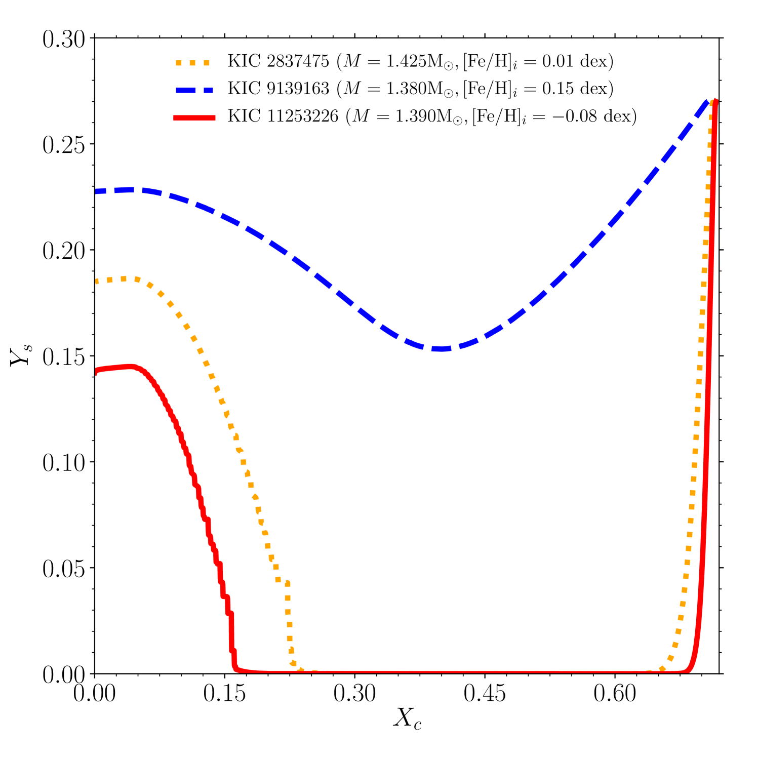
To demonstrate that the representative models of these stars with atomic diffusion predict large settling of the surface helium, we computed three tracks with the mass and metallicity from Table 1 (central value of the range for the mass). Figure 1 shows the evolution (from right-to-left) of the surface helium abundance, , for the tracks. We can see the complete depletion of for KIC 2839163 and 11253226 in the corresponding ranges listed in Table 1, making them ideal for this study. The track corresponding to KIC 9139163 does not show complete depletion of surface helium because of its large metallicity (and hence thick convective envelope), however as we shall see in Section 5, predicted settling is still too large for this star to reproduce the observed amplitude of helium signature.
3 Average amplitude of helium signature
There are two popular fitting approaches to extract the glitch signatures from the oscillation frequencies: (1) by fitting directly the oscillation frequencies (see e.g. Monteiro et al., 1994; Monteiro & Thompson, 1998; Monteiro et al., 2000), and (2) by fitting their second differences, , where and are the radial order and harmonic degree, respectively (see e.g. Gough, 1990; Basu et al., 1994; Basu et al., 2004). In this work, we used a variation of the first approach as described in Method A of Verma et al. (2017); Verma et al. (2019). It should be noted that the systematic uncertainties on the helium glitch parameters associated with different choices of fitting methods are generally small for stars in the LEGACY sample (Verma et al., 2019). This is because of the high-quality seismic data available for these stars with large numbers of detected modes and precisely measured oscillation frequencies. The precision of the observed oscillation frequencies of F stars is poor in comparison to other stars in the LEGACY sample because of their large linewidths (see e.g. Appourchaux et al., 2012; Lund et al., 2017; Compton et al., 2019), however their large amplitude of the helium signature effectively compensates for the lower precision.
For the convenience of the reader, we outline here the steps to calculate the average amplitude of helium signature. The stellar oscillation frequencies were fitted to the function,
| (1) |
The first (also the dominant) term represents the contribution to the oscillation frequency from the smooth structure of the star, which is modelled using -dependent fourth degree polynomial in (see e.g. Verma et al., 2019),
| (2) |
where are the polynomial coefficients to be determined by fitting to the oscillation frequencies. The second and third terms are small perturbations to frequencies due to the helium and base of convection zone glitches, respectively. The functional form for these contributions are adapted from Houdek & Gough (2007),
| (3) | |||||
| (4) |
where the parameters , , , , , and are free parameters to be again determined by fitting to the oscillation frequencies. We used Monte Carlo simulation to propagate the observational uncertainties on oscillation frequencies to the fitted parameters.
We used the fitted parameters, and , to compute the average amplitude of the helium signature (Verma et al., 2019),
| (5) | |||||
where and are the smallest and largest observed frequencies used in the fit. The same values of and have been consistently used to calculate the corresponding model .
4 Stellar models
We used the stellar evolution code Modules for Experiments in Stellar Astrophysics (MESA; Paxton et al., 2011; Paxton et al., 2013, 2015) to compute several grids of models with atomic diffusion and turbulence as competing process. The code was used with Opacity Project (OP) high-temperature opacities (Badnell et al., 2005; Seaton, 2005) supplemented with low-temperature opacities of Ferguson et al. (2005). The metallicity mixture from Grevesse & Sauval (1998) was used. We used OPAL equation of state (Rogers & Nayfonov, 2002). The reaction rates were from NACRE (Angulo et al., 1999) for all reactions except and , for which updated reaction rates from Imbriani et al. (2005) and Kunz et al. (2002) were used. We included settling of the helium and heavy elements following Thoul et al. (1994). We used an exponential overshoot at all possible radiative-convective boundaries (Herwig, 2000). The oscillation frequencies were calculated using the Adiabatic Pulsation code (ADIPLS; Christensen-Dalsgaard, 2008).
4.1 Turbulent diffusion
The stellar evolution code MESA provides a number of options for the input physics that the users can explore. For instance, it already implements a form of turbulent diffusion at the base of convection zone (see the module $MESA_DIR/star/private/turbulent_diffusion.f90 in the MESA package) to study the helium and heavy element settling in the Sun (Proffitt & Michaud, 1991). Moreover, it also ships a number of hooks with the package to enable the users conveniently implement certain type of new physics.
We used the already present turbulent diffusion for the Sun in MESA as a guide to implement the turbulent diffusion coefficient of Richer et al. (2000) for hotter stars. This was accomplished using the hook $MESA_DIR/star/other/other_d_mix.f90. We implemented the density-dependent diffusion coefficient,
| (6) |
where and are constants. Here, and are the density and atomic diffusion coefficient of helium at a reference depth, respectively. We used a simple analytical approximation for the atomic diffusion coefficient of helium following Richer et al. (2000),
| (7) |
where is the temperature. In earlier studies, reference depth in Eq. 6 was defined at either fixed or (see e.g. Richer et al., 2000), however the definition has been revised in recent studies as follows. Richer et al. (2000) noted that the surface element abundances depend only on the envelope mass mixed by turbulence (and not on the independent choices of , and reference depth). This led Michaud et al. (2011a, b) to cleverly redefine by fixing at 10000 and at 4 and anchoring the turbulent diffusion coefficient at a radial coordinate, , determined by a fixed outer mass, , where is the mass enclosed in a sphere of radius . This means that and in Eq. 6 are the density and atomic diffusion coefficient of helium at a depth corresponding to the outer mass of . Since the parameter determines the envelope mass mixed by turbulence (see e.g. Michaud et al., 2011b), it is referred as envelope mixed mass in the subsequent sections. Note that the envelope convection zone of F stars may be split into superficial convective regions due to opacity peaks in the ionization zones of helium and iron. The turbulent mixing was used at the base of every such region, resulting complete mixing of radiative layers between superficial convection zones, as expected from the results of numerical simulations (see e.g. Kupka & Montgomery, 2002; Freytag & Steffen, 2004).
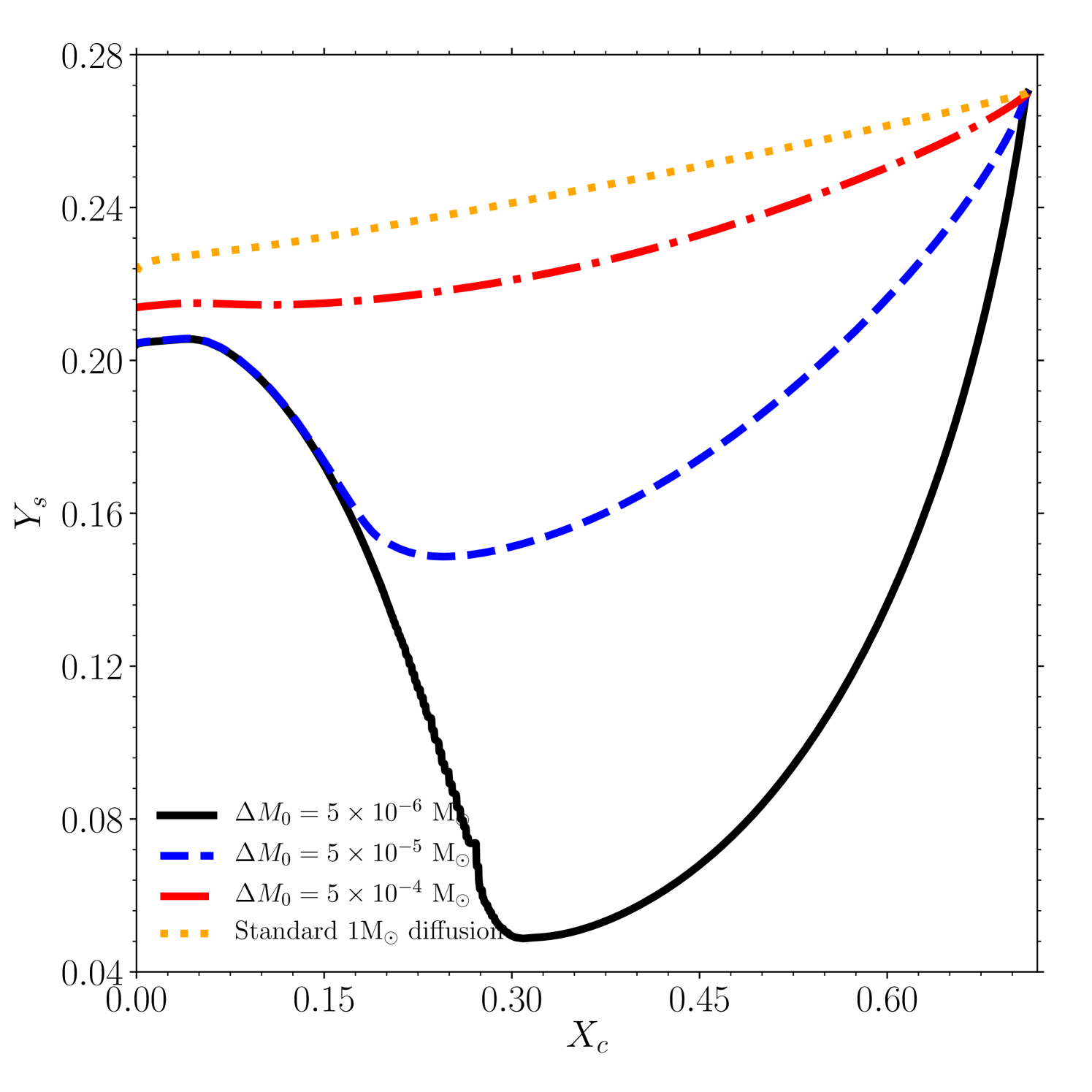
Figure 2 shows evolution of the surface helium abundance for models in three tracks with M⊙. All three tracks were computed with mass M⊙. We can see that as increases, the amount of helium settling on the MS decreases. The models of atomic diffusion have been thoroughly tested for the Sun using helioseismic data, and are known to predict helium and heavy element settling reasonably well without any additional mixing. Figure 2 also shows a solar-mass track without turbulent mixing for comparison. We note that the track with M⊙ is closest to the solar-mass track.
| KIC | (M⊙) | ||||||
|---|---|---|---|---|---|---|---|
| M⊙ | M⊙ | M⊙ | |||||
| 2837475 | |||||||
| 9139163 | |||||||
| 11253226 | |||||||
It is clear from Eq. 6 that decreases very rapidly as we move inward from the anchor point because of the increase in density. This means that if the anchor point falls well within the envelope convection zone, i.e. , then the turbulent mixing has very little impact at the base of convection zone. Since the low-mass models have thick convective envelope, the inclusion of turbulence has insignificant impact on their structure (as desired for the Sun). The evolution of the surface helium abundance for the solar-mass track with atomic diffusion and turbulence falls exactly on the dotted curve in Figure 2 (not shown for clarity). This opens a possibility for the future to consistently use atomic diffusion with turbulence while modelling both low and high-mass stars, reducing the systematic uncertainties on the inferred stellar properties associated with the arbitrary transition from diffusion models for low-mass stars to non-diffusion models for high-mass stars.
4.2 Model grids
We constructed three grids of models for each star with three values of the envelope mixed mass, M⊙. For each grid, we computed 50 tracks – each containing hundreds of models on the MS – sampling uniformly using quasi-random numbers (more specifically using Sobol sequences) the 5-D space formed by mass , initial metallicity , initial helium abundance , mixing-length and overshoot . Note that we do not need very dense grid of models like we do when modelling stars. The goal here is to explore the likely parameter space of stars in the sample to see if we can reproduce the observed amplitude of helium signature. Table 2 lists the parameter spaces considered for each grid of stars in the sample. The range in was shifted to higher values in comparison to the observed to compensate for element settling. Note that the shift depends on the value of and was estimated by trying different values of and comparing the predicted with the corresponding observed value for each . Since smaller value of means larger settling of the helium and heavy elements on the MS, the shift is larger for the grid with M⊙ in comparison to M⊙.
We find a representative model of a star from a given track by fitting the surface corrected model frequencies (Kjeldsen et al., 2008) to the observed ones. As discussed in Verma et al. (2019), the choice of the surface correction scheme is not important for this particular exercise because, for a given track, the age can be determined very precisely by fitting the observed oscillation frequencies irrespective of the surface correction used. In this manner, we get 50 representative models of a star from each grid.
5 Results
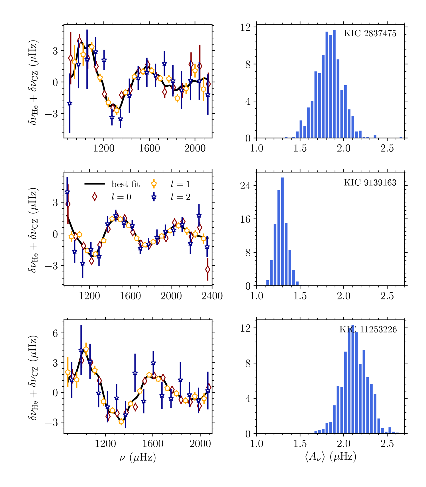
We fitted the observed oscillation frequencies of each star using the method outlined in Section 3 to extract the glitch signatures. The left panels in Figure 3 show the fit to the observed oscillation frequencies of KIC 2837475, 9139163 and 11253226 (top-to-bottom) after removing the smooth component, . The smooth component was subtracted to clearly see the glitch signatures. The signature with large amplitude and large period is from the helium ionization zone while the modulation on top of it with small amplitude and small period is from the base of convection zone. The right panels in the figure show the distribution of the observed average amplitude of the helium glitch signature obtained using Monte Carlo simulation. The unimodal nature of the distribution shows the robustness of the fit. As discussed in Section 3, we can see the large average amplitude of the helium signature (>1Hz) for these stars in comparison to the other cool stars in the LEGACY sample (<1Hz; see Table 1 of Verma et al. (2017)).
As discussed in Section 4, we have three sets of 50 representative models of each star with three different values of the envelope mixed mass, M⊙. We fitted the frequencies of all the representative models to extract the glitch signatures. To avoid systematic uncertainties, the fit was performed using the same set of modes and weights as for the observations. We used the fitted parameters for all the models to calculate the corresponding average amplitude of the helium signature using Eq. 5.
5.1 Comparison of the observed and model amplitudes
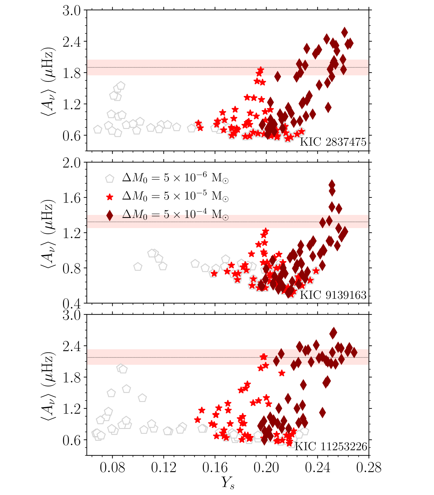
We compare in Figure 4 the observed average amplitude of the helium signature with those predicted by the representative models of different envelope mixed mass. First, we shall look at the models with M⊙. In all three stars it can be seen that for most of the representative models is small because of the large helium settling. The small introduces a weak helium glitch in the acoustic structure, leaving a weak helium signature in the model frequencies. Consequently, the average amplitude is smaller for all models in comparison to the observed . This led us to conclude that must be greater than M⊙ to reduce further the helium settling.
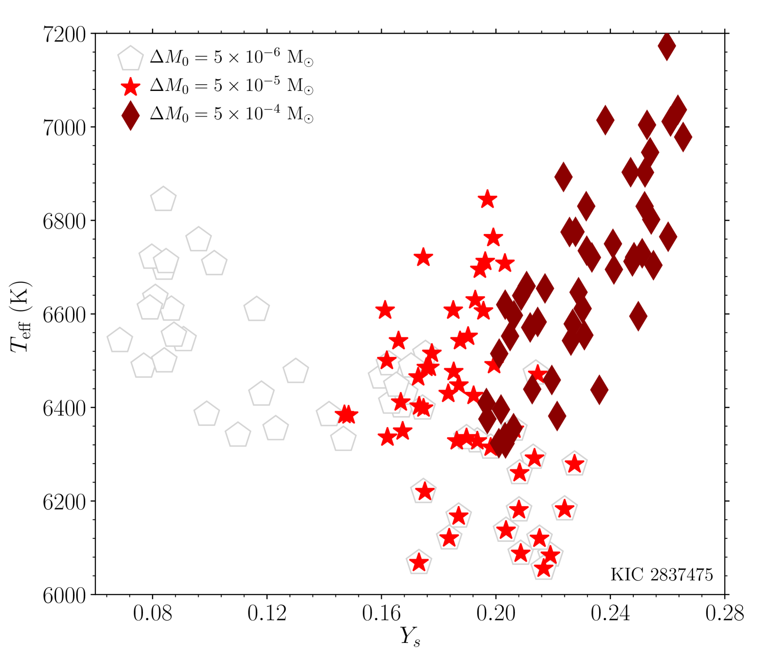
In Figure 4, it is interesting to note the behaviour of as a function of for the models with M⊙; it decreases slightly instead of increasing as increases. This is because, it turns out that the models with smaller have larger for M⊙, as can be seen in Figure 5. The average amplitude is known to rapidly increase as increases (see Figure 6 of Verma et al., 2014b). Hence, the effect of the decrease in on gets compensated by the increase in , resulting in the trend seen in the figure.
As we can see in Figure 4, most of the models (all for KIC 9139163) with M⊙ have systematically lower average amplitude than the corresponding observed . This suggests that these models are also unlikely to represent the stars, though we can not completely disregard the possibility yet. The models with M⊙, however, show the familiar trend, i.e. increases as increases. These models do reproduce the observed for certain value of .
We note that the scatter in Figure 4 for a given is intrinsic and due to differences in , , , and age. Although correlates with other stellar parameters such as age, the correlation can mostly be explained by the dependence of the corresponding parameter on and (see Figure 7 of Verma et al., 2014a). Moreover, we constructed grids with broad ranges in stellar parameters (for an example, models between the ZAMS and the TAMS were considered) in order to avoid any possible biases (for an example, related to the uncertainties in the evolutionary stage of the targets).
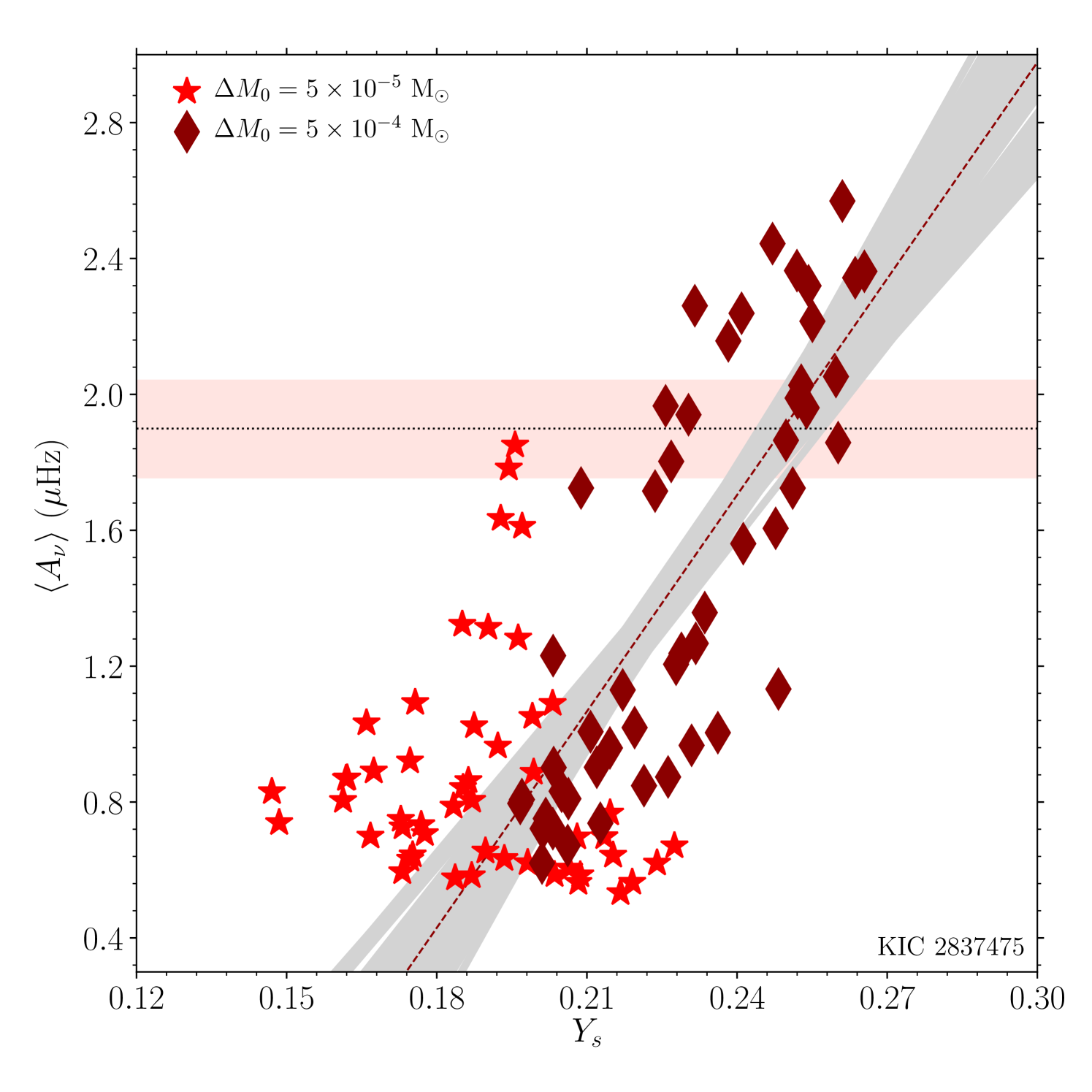
In Figure 6, we note that the models with M⊙ put together show a reasonably tight correlation between and . We calibrated the observed against these models of different to infer the surface helium abundance for all three stars. To perform the calibration, we fitted a straight line to the model as a function of . Since the models with M⊙ are unlikely to represent the stars and may potentially bias the helium estimate, we gave less weight to these models in the fit. The trial and error method suggested a reasonable choice of one-fourth of the weight given to the models with M⊙. The intersection of the fitted line and the horizontal line corresponding to the observed provided of , and for KIC 2837475, 9139163 and 11253226, respectively.
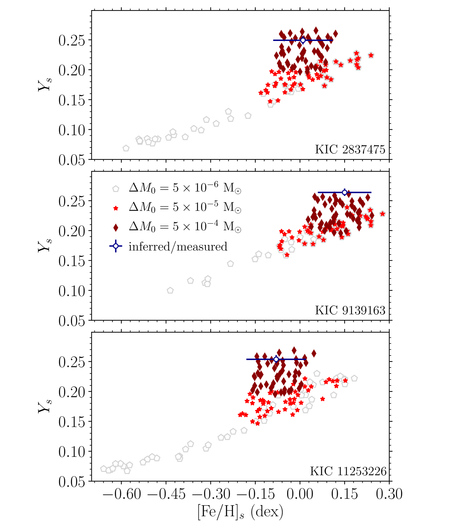
In Figure 7, we compare simultaneously the inferred and measured of all stars with the corresponding quantities predicted by the representative models with different values of . We can see that only the models with M⊙ reproduce both quantities together. This led us to conclude that we need turbulent mixing with approximately M⊙ to reproduce the observed .
5.2 Comparison of the observed and model acoustic depths
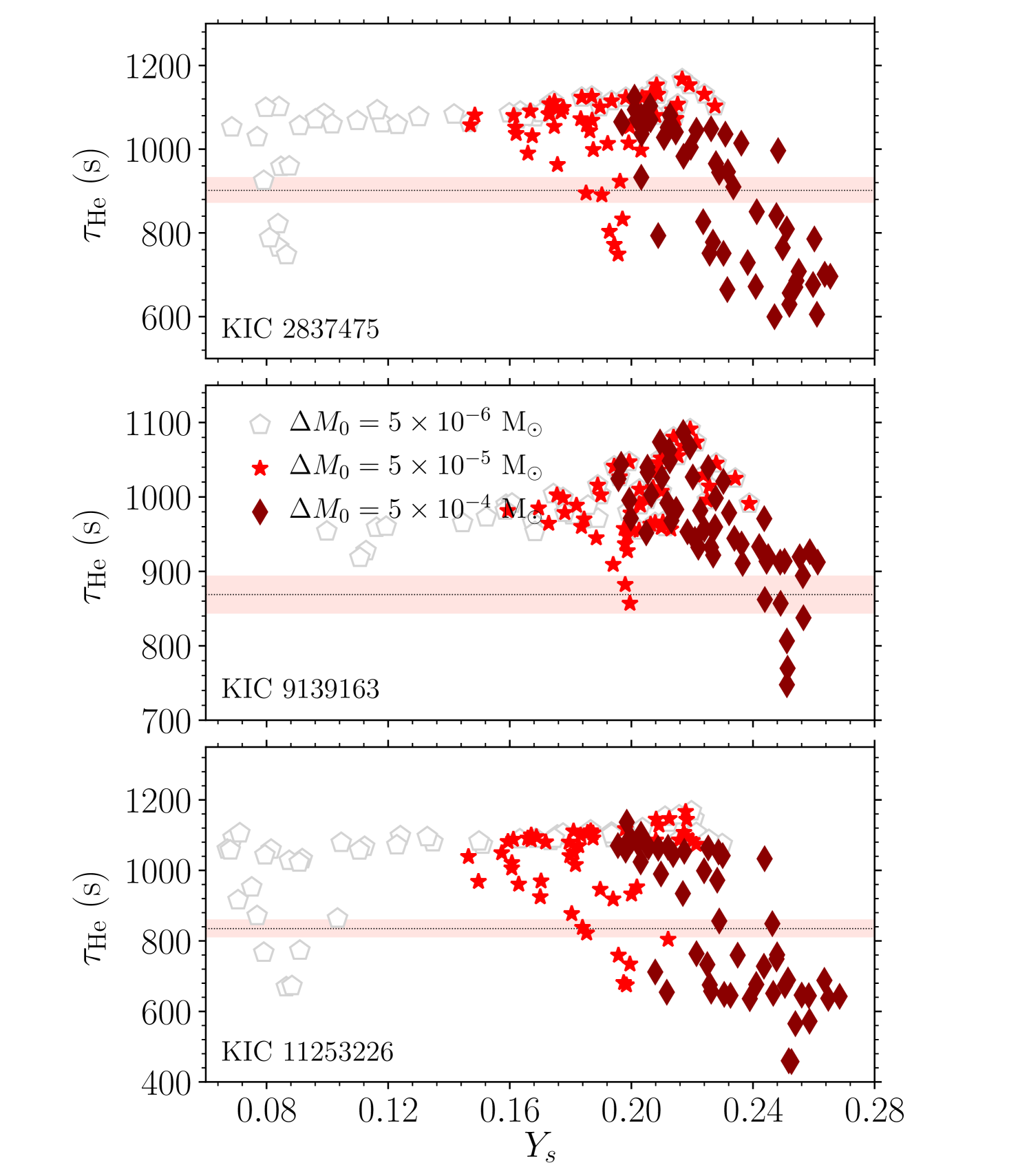
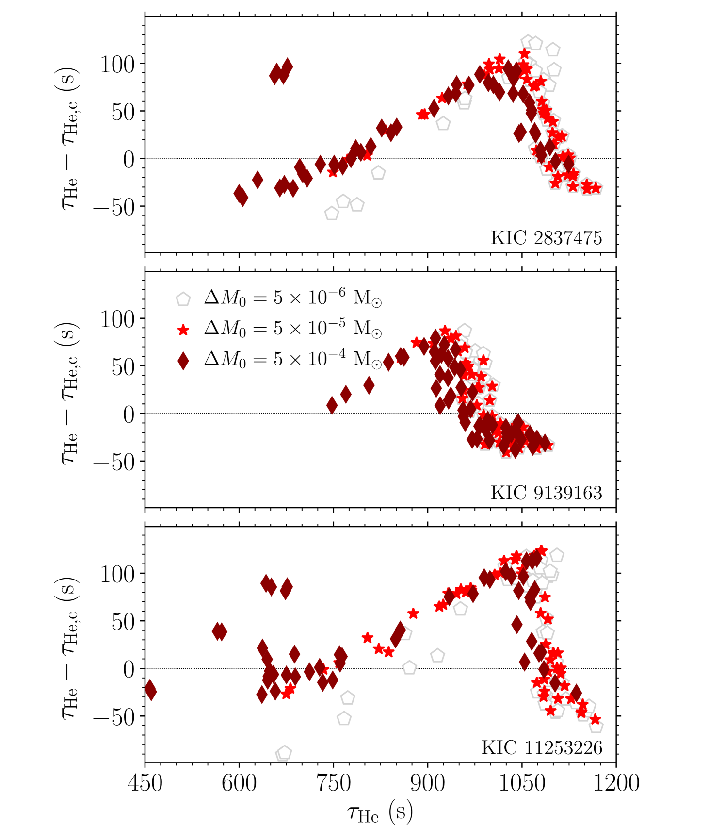
We now compare the acoustic depth of the helium ionization zone obtained by fitting the observed oscillation frequencies with those obtained by fitting the model frequencies of different envelope mixed mass. As we can see in Figure 8 for all three stars, most of the models with M⊙ have systematically larger than the corresponding observed . Since the acoustic depth of a layer depends on the sound speed of layers above it (see Eq. 8), most of these models have systematically different sound speed in the outer layers compared to the star. Again, models with M⊙ have on both side of the observed . This reinforces the conclusion that we need turbulent mixing with approximately M⊙.
5.3 Sanity check for the model fits
Fitting the oscillation frequencies to function involves non-linear optimization in a high-dimensional space, and fits may not necessarily converge for all models. Since we have a large number of models, it is not feasible to examine the fits to the model frequencies visually as we do for the fits to the observed frequencies. We do, however, perform a sanity check by comparing the fitted acoustic depth of helium ionization zone ( in Eq. 3) with that obtained using sound speed, , of the model. Using sound speed profile of the model, we can compute the acoustic depth of helium ionization zone,
| (8) |
where and are the radial coordinates of the acoustic surface and helium ionization zone, respectively.
The comparison between and is known to be ambiguous for two reasons. First, the definition of the acoustic surface is uncertain, and is typically defined as a point in the atmosphere where the linear extrapolation of from outermost convective layers vanishes (Balmforth & Gough, 1990). This point falls at an acoustic height of approximately 225s from the photosphere for the Sun (see e.g. Houdek & Gough, 2007). Assuming that the “true" acoustic surface lies between the photosphere and the point where extrapolated vanishes, a maximum systematic uncertainty of 225s is expected on for the Sun. Since we only used for sanity check of the fits, we simplistically assumed the radial coordinate of the outermost layer in the model at an optical depth of for . Secondly, the definition of in Eq. 8 is also uncertain, introducing an additional systematic uncertainty on . It has recently been shown that the helium glitch signature arises from a region close to the peak in the first adiabatic index, , between the first and second helium ionization zones (Broomhall et al., 2014; Verma et al., 2014b). We used the radial coordinate of the -peak for .
Figure 9 shows the absolute difference between and for all representative models of all three stars. As we can see, the differences are much smaller than the maximum possible systematic uncertainty expected from the uncertainties in the definitions of and , reassuring the quality of the fits and conclusions of the paper.
6 Discussion and Conclusions
We identified three stars, KIC 2837475, 9139163 and 11253226, from the Kepler asteroseismic LEGACY sample for which the standard models of atomic diffusion predict large settling (or complete depletion) of the surface helium. We extracted the oscillatory signature of helium ionization from the observed oscillation frequencies. The detection of a strong helium signature in these stars already indicates the presence of significant amount of helium in their envelope, in contrast to what we would anticipate if atomic diffusion is the only process determining the surface helium abundance. This confirms the presence of additional physical processes competing against atomic diffusion.
In the current study, we assumed turbulence to be the only process that slows down the settling of helium. Since radiative acceleration for helium is much smaller than gravitational acceleration (see e.g. Richer et al., 2000), radiative forces have negligible effect on the surface helium abundance. The inclusion of radiative forces in the current analysis is only expected to reduce the shift necessary in to compensate for element settling. The advantage of excluding radiative forces is that the detailed grid-based modelling taking uncertainties in stellar properties into account becomes computationally feasible.
We implemented in MESA the phenomenological turbulent diffusion coefficient of Richer et al. (2000) in a form described in Michaud et al. (2011a, b). In this formalism, the surface abundances depend only on one parameter, , which is related to the mass mixed by turbulence in the envelope. We computed three grids of models with M⊙ for each star, and identified 50 representative models of the star from each grid. Subsequently, we extracted the helium signature from the oscillation frequencies of representative models, and computed the corresponding average amplitude. For all three stars, models with M⊙ have too low average amplitude of helium signature because of the large helium settling to reproduce the observed . We found that the models with M⊙ have average amplitude consistent with the observations.
Previous studies using measurements of heavy element abundances and stellar models with atomic diffusion, radiative forces and turbulence suggested an envelope mixed mass of approximately M⊙ (see e.g. Michaud et al., 2011b). This is too small to reproduce the surface helium abundance. This clearly demonstrates the potential of using the spectroscopically measured elemental abundances together with the seismic constraint of helium abundance to discriminate among the different possible physical processes competing against atomic diffusion. A systematic study in this direction using the seismic constraint of helium abundance and the spectroscopic measurements of the heavy element abundances together with the state-of-the-art stellar models including atomic diffusion, radiative forces, turbulence, mass loss, etc. can help us identify the most important physical processes competing against atomic diffusion, leading to the correct interpretation of the observed surface abundances of hot stars, consistent use of atomic diffusion for modelling both hot and cool stars reducing the systematic uncertainties on the inferred stellar properties and shed some light on the long-standing cosmological lithium problem.
Acknowledgements
Funding for the Stellar Astrophysics Centre is provided by The Danish National Research Foundation (Grant agreement no.: DNRF106). We thank the anonymous referee for constructive feedback. We thank J. Christensen-Dalsgaard and G. Houdek for carefully reading the manuscript. KV would like to thank S. Hanasoge for kindly providing the time on SEISMO-cluster in the beginning of the project. VSA acknowledges support from the Independent Research Fund Denmark (Research grant 7027-00096B).
References
- Aller & Chapman (1960) Aller L. H., Chapman S., 1960, ApJ, 132, 461
- Angulo et al. (1999) Angulo C., et al., 1999, Nuclear Physics A, 656, 3
- Appourchaux et al. (2012) Appourchaux T., et al., 2012, A&A, 543, A54
- Badnell et al. (2005) Badnell N. R., Bautista M. A., Butler K., Delahaye F., Mendoza C., Palmeri P., Zeippen C. J., Seaton M. J., 2005, MNRAS, 360, 458
- Bahcall et al. (1997) Bahcall J. N., Pinsonneault M. H., Basu S., Christensen-Dalsgaard J., 1997, Physical Review Letters, 78, 171
- Balmforth & Gough (1990) Balmforth N. J., Gough D. O., 1990, ApJ, 362, 256
- Basu et al. (1994) Basu S., Antia H. M., Narasimha D., 1994, MNRAS, 267, 209
- Basu et al. (2004) Basu S., Mazumdar A., Antia H. M., Demarque P., 2004, MNRAS, 350, 277
- Bertelli Motta et al. (2018) Bertelli Motta C., et al., 2018, MNRAS, 478, 425
- Broomhall et al. (2014) Broomhall A.-M., et al., 2014, MNRAS, 440, 1828
- Chapman (1917a) Chapman S., 1917a, MNRAS, 77, 539
- Chapman (1917b) Chapman S., 1917b, MNRAS, 77, 540
- Chapman (1922) Chapman S., 1922, MNRAS, 82, 292
- Christensen-Dalsgaard (2008) Christensen-Dalsgaard J., 2008, Ap&SS, 316, 113
- Christensen-Dalsgaard et al. (1993) Christensen-Dalsgaard J., Proffitt C. R., Thompson M. J., 1993, ApJ, 403, L75
- Compton et al. (2019) Compton D. L., Bedding T. R., Stello D., 2019, MNRAS, 485, 560
- Deal et al. (2018) Deal M., Alecian G., Lebreton Y., Goupil M. J., Marques J. P., LeBlanc F., Morel P., Pichon B., 2018, A&A, 618, A10
- Dotter et al. (2017) Dotter A., Conroy C., Cargile P., Asplund M., 2017, ApJ, 840, 99
- Ferguson et al. (2005) Ferguson J. W., Alexander D. R., Allard F., Barman T., Bodnarik J. G., Hauschildt P. H., Heffner-Wong A., Tamanai A., 2005, ApJ, 623, 585
- Freytag & Steffen (2004) Freytag B., Steffen M., 2004, in Zverko J., Ziznovsky J., Adelman S. J., Weiss W. W., eds, IAU Symposium Vol. 224, The A-Star Puzzle. pp 139–147, doi:10.1017/S174392130400448X
- Gai et al. (2018) Gai N., Basu S., Tang Y., 2018, ApJ, 856, 123
- Gough (1990) Gough D. O., 1990, in Osaki Y., Shibahashi H., eds, Lecture Notes in Physics, Berlin Springer Verlag Vol. 367, Progress of Seismology of the Sun and Stars. p. 283, doi:10.1007/3-540-53091-6
- Gough & Thompson (1988) Gough D. O., Thompson M. J., 1988, in Christensen-Dalsgaard J., Frandsen S., eds, IAU Symposium Vol. 123, Advances in Helio- and Asteroseismology. p. 155
- Grevesse & Sauval (1998) Grevesse N., Sauval A. J., 1998, Space Sci. Rev., 85, 161
- Gruyters et al. (2013) Gruyters P., Korn A. J., Richard O., Grundahl F., Collet R., Mashonkina L. I., Osorio Y., Barklem P. S., 2013, A&A, 555, A31
- Gruyters et al. (2014) Gruyters P., Nordlander T., Korn A. J., 2014, A&A, 567, A72
- Herwig (2000) Herwig F., 2000, A&A, 360, 952
- Houdek (2004) Houdek G., 2004, in Celebonovic V., Gough D., Däppen W., eds, American Institute of Physics Conference Series Vol. 731, Equation-of-State and Phase-Transition in Models of Ordinary Astrophysical Matter. pp 193–207, doi:10.1063/1.1828405
- Houdek & Gough (2007) Houdek G., Gough D. O., 2007, MNRAS, 375, 861
- Imbriani et al. (2005) Imbriani G., et al., 2005, European Physical Journal A, 25, 455
- Kjeldsen et al. (2008) Kjeldsen H., Bedding T. R., Christensen-Dalsgaard J., 2008, ApJ, 683, L175
- Korn et al. (2006) Korn A. J., Grundahl F., Richard O., Barklem P. S., Mashonkina L., Collet R., Piskunov N., Gustafsson B., 2006, Nature, 442, 657
- Korn et al. (2007) Korn A. J., Grundahl F., Richard O., Mashonkina L., Barklem P. S., Collet R., Gustafsson B., Piskunov N., 2007, ApJ, 671, 402
- Kunz et al. (2002) Kunz R., Fey M., Jaeger M., Mayer A., Hammer J. W., Staudt G., Harissopulos S., Paradellis T., 2002, ApJ, 567, 643
- Kupka & Montgomery (2002) Kupka F., Montgomery M. H., 2002, MNRAS, 330, L6
- Lind et al. (2008) Lind K., Korn A. J., Barklem P. S., Grundahl F., 2008, A&A, 490, 777
- Lund et al. (2017) Lund M. N., et al., 2017, ApJ, 835, 172
- Mazumdar et al. (2014) Mazumdar A., et al., 2014, ApJ, 782, 18
- Michaud & Charland (1986) Michaud G., Charland Y., 1986, ApJ, 311, 326
- Michaud et al. (1983) Michaud G., Tarasick D., Charland Y., Pelletier C., 1983, ApJ, 269, 239
- Michaud et al. (2011a) Michaud G., Richer J., Richard O., 2011a, A&A, 529, A60
- Michaud et al. (2011b) Michaud G., Richer J., Vick M., 2011b, A&A, 534, A18
- Monteiro & Thompson (1998) Monteiro M. J. P. F. G., Thompson M. J., 1998, in Deubner F.-L., Christensen-Dalsgaard J., Kurtz D., eds, IAU Symposium Vol. 185, New Eyes to See Inside the Sun and Stars. p. 317
- Monteiro & Thompson (2005) Monteiro M. J. P. F. G., Thompson M. J., 2005, MNRAS, 361, 1187
- Monteiro et al. (1994) Monteiro M. J. P. F. G., Christensen-Dalsgaard J., Thompson M. J., 1994, A&A, 283, 247
- Monteiro et al. (2000) Monteiro M. J. P. F. G., Christensen-Dalsgaard J., Thompson M. J., 2000, MNRAS, 316, 165
- Morel & Thévenin (2002) Morel P., Thévenin F., 2002, A&A, 390, 611
- Nordlander et al. (2012) Nordlander T., Korn A. J., Richard O., Lind K., 2012, ApJ, 753, 48
- Paxton et al. (2011) Paxton B., Bildsten L., Dotter A., Herwig F., Lesaffre P., Timmes F., 2011, ApJS, 192, 3
- Paxton et al. (2013) Paxton B., et al., 2013, ApJS, 208, 4
- Paxton et al. (2015) Paxton B., et al., 2015, ApJS, 220, 15
- Proffitt & Michaud (1991) Proffitt C. R., Michaud G., 1991, ApJ, 380, 238
- Richard et al. (1996) Richard O., Vauclair S., Charbonnel C., Dziembowski W. A., 1996, A&A, 312, 1000
- Richer et al. (2000) Richer J., Michaud G., Turcotte S., 2000, ApJ, 529, 338
- Rogers & Nayfonov (2002) Rogers F. J., Nayfonov A., 2002, ApJ, 576, 1064
- Schatzman (1969) Schatzman E., 1969, A&A, 3, 331
- Seaton (2005) Seaton M. J., 2005, MNRAS, 362, L1
- Silva Aguirre et al. (2017) Silva Aguirre V., et al., 2017, ApJ, 835, 173
- Thoul et al. (1994) Thoul A. A., Bahcall J. N., Loeb A., 1994, ApJ, 421, 828
- Turcotte et al. (1998) Turcotte S., Richer J., Michaud G., 1998, ApJ, 504, 559
- Varenne & Monier (1999) Varenne O., Monier R., 1999, A&A, 351, 247
- Vauclair et al. (1978a) Vauclair S., Vauclair G., Schatzman E., Michaud G., 1978a, ApJ, 223, 567
- Vauclair et al. (1978b) Vauclair G., Vauclair S., Michaud G., 1978b, ApJ, 223, 920
- Verma et al. (2014a) Verma K., et al., 2014a, ApJ, 790, 138
- Verma et al. (2014b) Verma K., Antia H. M., Basu S., Mazumdar A., 2014b, ApJ, 794, 114
- Verma et al. (2017) Verma K., Raodeo K., Antia H. M., Mazumdar A., Basu S., Lund M. N., Silva Aguirre V., 2017, ApJ, 837, 47
- Verma et al. (2019) Verma K., Raodeo K., Basu S., Silva Aguirre V., Mazumdar A., Mosumgaard J. R., Lund M. N., Ranadive P., 2019, MNRAS, 483, 4678
- Vick et al. (2010) Vick M., Michaud G., Richer J., Richard O., 2010, A&A, 521, A62
- Vorontsov (1988) Vorontsov S. V., 1988, in Christensen-Dalsgaard J., Frandsen S., eds, IAU Symposium Vol. 123, Advances in Helio- and Asteroseismology. p. 151