Hidden-charm pentaquarks with triple strangeness due to the interactions
Abstract
Motivated by the successful interpretation of these observed and states under the meson-baryon molecular picture, we systematically investigate the possible hidden-charm molecular pentaquark states with triple strangeness which is due to the interactions. We perform a dynamical calculation of the possible hidden-charm molecular pentaquarks with triple strangeness by the one-boson-exchange model, where the - wave mixing effect and the coupled channel effect are taken into account in our calculation. Our results suggest that the state with and the state with can be recommended as the candidates of the hidden-charm molecular pentaquark with triple strangeness. Furthermore, we discuss the two-body hidden-charm strong decay behaviors of these possible hidden-charm molecular pentaquarks with triple strangeness by adopting the quark-interchange model. These predictions are expected to be tested at the LHCb, which can be as a potential research issue with more accumulated experimental data in near future.
I Introduction
As is well known, the study of the matter spectrum is an important way to explore the relevant matter structures and the involved interaction properties. In the hadron physics, since the discovery of the by the Belle Collaboration Choi:2003ue , a series of exotic states has been observed benefiting from the accumulation of more and more experimental data with high precision, and the exotic hadrons have stimulated extensive studies in the past two decades (see the review articles Chen:2016qju ; Liu:2019zoy ; Olsen:2017bmm ; Guo:2017jvc ; Liu:2013waa ; Hosaka:2016pey ; Brambilla:2019esw for learning the relevant processes). Exploring these exotic hadronic states not only gives new insights for revealing the hadron structures, but also provides useful hints to deepening our understanding of the nonperturbative behavior of the quantum chromodynamics (QCD) in the low energy regions.
In fact, investigating the pentaquark states has been a long history, which can be tracked back to the birth of the quark model GellMann:1964nj ; Zweig:1981pd . Among exotic hadronic states, the hidden-charm molecular pentaquarks have attracted much attention as early as 2010 Li:2014gra ; Karliner:2015ina ; Wu:2010jy ; Wang:2011rga ; Yang:2011wz ; Wu:2012md ; Chen:2015loa and become a hot topic with the discovery of the and in the process by the LHCb Collaboration Aaij:2015tga . In 2019, there was a new progress about the observation of three narrow structures [, , and ] by revisiting the process based on more collected data Aaij:2019vzc , and they are just below the corresponding thresholds of the -wave charmed baryon and -wave anticharmed meson. This provides strong evidence to support the existence of the hidden-charm meson-baryon molecular states. More recently, the LHCb Collaboration reported a possible hidden-charm pentaquark with strangeness Aaij:2020gdg , and this structure can be assigned as the molecular state Chen:2016ryt ; Wu:2010vk ; Hofmann:2005sw ; Anisovich:2015zqa ; Wang:2015wsa ; Feijoo:2015kts ; Lu:2016roh ; Xiao:2019gjd ; Shen:2020gpw ; Chen:2015sxa ; Zhang:2020cdi ; Wang:2019nvm ; Chen:2020uif ; Peng:2020hql ; 1830432 ; 1830426 ; Liu:2020hcv ; 1839195 .
Facing the present status of exploring the hidden-charm molecular pentaquarks Chen:2016qju ; Liu:2019zoy ; Olsen:2017bmm ; Guo:2017jvc , we naturally propose a meaningful question: why are we interested in the hidden-charm molecular pentaquark states? The hidden-charm pentaquark states are relatively easy to produce via the bottom baryon weak decays in the experimental facilities Aaij:2019vzc ; Aaij:2020gdg , and the hidden-charm quantum number is a crucial condition for the existence of the hadronic molecules Li:2014gra ; Karliner:2015ina . In addition, it is worth indicating that the heavy hadrons are more likely to generate the bound states due to the relatively small kinetic terms, and the interactions between the charmed baryon and the anticharmed meson may be mediated by exchanging a series of allowed light mesons Chen:2016qju ; Liu:2019zoy . Indeed, these announced hidden-charm pentaquark states have a () pair Chen:2016qju ; Liu:2019zoy ; Olsen:2017bmm ; Guo:2017jvc .
Based on the present research progress on the hidden-charm pentaquarks Chen:2016qju ; Liu:2019zoy ; Olsen:2017bmm ; Guo:2017jvc , the theorists should pay more attention to making the reliable prediction of various types of the hidden-charm molecular pentaquarks and give more abundant suggestions to searching for the hidden-charm molecular pentaquarks accessible at the forthcoming experiment. Generally speaking, there are two important approaches to construct the family of the hidden-charm molecular pentaquark states which is very special in the hadron spectroscopy. Firstly, we propose that there may exist a series of hidden-charm molecular pentaquarks with the different strangeness. Secondly, we also have enough reason to believe that there may exist more hidden-charm molecular pentaquark states with higher mass. In fact, we already studied the systems with double strangeness Wang:2020bjt and the systems with and Wang:2019nwt , and predicted a series of possible candidates of the hidden-charm molecular pentaquarks. In fact, the triple-strangeness hidden-charm pentaquarks may be regarded as systems that can be used to reveal the binding mechanism and the importance of the scalar-meson exchange as they are not expected to exist in the treatment of Ref. 1839195 . Thus, we investigate the possible hidden-charm molecular pentaquarks with triple strangeness from the interactions, which will be a main task of the present work.
In the present work, we perform a dynamical calculation with the possible hidden-charm molecular pentaquark states with triple strangeness by adopting the one-boson-exchange (OBE) model Chen:2016qju ; Liu:2019zoy , which involves the interactions between an -wave charmed baryon and an -wave anticharmed-strange meson . In concrete calculation, the - wave mixing effect and the coupled channel effect are taken into account. Furthermore, we study the two-body hidden-charm strong decay behaviors of these possible hidden-charm molecular pentaquarks. Here, we adopt the quark-interchange model to estimate the transition amplitudes for the decay widths Barnes:1991em ; Barnes:1999hs ; Barnes:2000hu , which is widely used to give the decay information of the exotic hadronic states during the last few decades Wang:2018pwi ; Wang:2019spc ; Xiao:2019spy ; Wang:2020prk ; Hilbert:2007hc . We hope that the present investigation is a key step to complement the family of the hidden-charm molecular pentaquark state and may provide crucial information of searching for possible hidden-charm molecular pentaquarks with triple strangeness. With higher statistic data accumulation at Run III of the LHC and after High-Luminosity-LHC upgrade Bediaga:2018lhg , it is highly probable that these possible hidden-charm molecular pentaquarks with triple strangeness can be detected at the LHCb Collaboration in the near future, which will be full of opportunities and challenges.
The remainder of this paper is organized as follows. In Sec. II, we introduce how to deduce the effective potentials and present the bound state properties of these investigated systems. We present the quark-interchange model and the two-body strong decay behaviors of these possible molecular pentaquarks in Sec. III. Finally, a short summary follows in Sec. IV.
II The interactions
II.1 OBE effective potentials
In the present work, we study the interactions between an -wave charmed baryon and an -wave anticharmed-strange meson . Here, we adopt the OBE model Chen:2016qju ; Liu:2019zoy , and consider the effective potentials from the , , and exchanges. In particular, we need to emphasize that the light scalar meson exchange provides effective interaction for these investigated systems, and we do not consider the and exchanges in our calculation, since the is usually considered as a meson with only up and down quarks and the is the light isovector scalar meson. In this subsection, we construct the relevant wave functions and effective Lagrangians, and deduce the OBE effective potentials in the coordinate space for all of the investigated systems.
Firstly, we introduce the flavor and spin-orbital wave functions involved in our calculation. For the systems, the flavor wave function is quite simple and reads as , where and are the isospin and its third component of the discussed system. In addition, the spin-orbital wave functions for these investigated systems are explicitly written as
In the above expressions, , , and denote the spin, orbit angular momentum, and total angular momentum for the discussed system, respectively. The constant is the Clebsch-Gordan coefficient, and is the spherical harmonics function. In the static limit, the polarization vector with the spin-1 field can be expressed as and . stands for the spin wave function of the charmed baryon with spin , and the polarization tensor of the charmed baryon with spin quantum number can be written in a general form, i.e.,
| (2.2) |
In order to write out the relevant scattering amplitudes quantitatively, we usually adopt the effective Lagrangian approach. To be convenient, we construct two types of super-fields and via the heavy quark limit Wise:1992hn . The superfield is expressed as a combination of the charmed baryons with and with in the flavor representation Chen:2017xat , and the superfield includes the anticharmed-strange vector meson with and the pseudoscalar meson with Ding:2008gr . The general expressions of the super-fields and can be given by
| (2.3) |
Here, is the four velocity under the nonrelativistic approximation.
With the above preparation, we construct the relevant effective Lagrangians to describe the interactions among the heavy hadrons and the light scalar, pseudoscalar, or vector mesons as Ding:2008gr ; Chen:2017xat
| (2.4) | |||||
which satisfy the requirement of the heavy quark symmetry, the chiral symmetry, and the hidden local symmetry Casalbuoni:1992gi ; Casalbuoni:1996pg ; Yan:1992gz ; Harada:2003jx ; Bando:1987br . The axial current and the vector current can be defined as and , respectively. Here, the pseudo-Goldstone field can be written as , where is the pion decay constant. In the above formulas, the vector meson field and its strength tensor are and , respectively. Here, , , and are the matrices of the charmed baryon in the flavor representation, light vector meson, and light pseudoscalar meson, which can be written as
| (2.17) |
respectively. By expanding the compact effective Lagrangians to the leading order of the pseudo-Goldstone field , we can further obtain the concrete effective Lagrangians. The effective Lagrangians for and the light mesons are expressed as
| (2.18) | |||||
| (2.19) | |||||
| (2.20) | |||||
and the effective Lagrangians to describe the -wave anticharmed-strange mesons and the light scalar, pseudoscalar, or vector mesons are
| (2.21) | |||||
| (2.22) | |||||
In the above effective Lagrangians, the coupling constants can be either extracted from the experimental data or calculated by the theoretical models, and the signs of these coupling constants are fixed via the quark model Riska:2000gd . The values of these coupling constants are , ,222In this work, we consider the contribution from light scalar meson exchange. Here, the corresponding coupling constant involved in effective Lagrangians [Eq. (2.18) and Eq. (2.21)] is approximately taken as the same as that for the case of light scalar . , , , , , , and Chen:2019asm , which are widely used to discuss the hadronic molecular states Wang:2020bjt ; Chen:2017xat ; Wang:2019nwt ; Chen:2019asm ; He:2015cea ; He:2019ify ; Chen:2018pzd . In particular, we need to emphasize that these input coupling constants can well reproduce the masses of the , , and Aaij:2019vzc under the meson-baryon molecular picture when adopting the OBE model Chen:2019asm ; He:2019ify .
We follow the standard strategy to deduce the effective potentials in the coordinate space in Refs. Wang:2020dya ; Wang:2019nwt ; Wang:2019aoc , which is a lengthy and tedious calculation. In Fig. 1, we present the relevant Feynman diagram for the scattering processes.
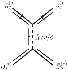
At the hadronic level, we firstly write out the scattering amplitude of the scattering process by considering the effective Lagrangian approach. And then, the effective potential in momentum space can be related to the scattering amplitude with the help of the Breit approximation Breit:1929zz ; Breit:1930zza and the nonrelativistic normalization, i.e.,
| (2.24) |
where and are the masses of the initial states and final states , respectively. By performing the Fourier transformation, the effective potential in the coordinate space can be deduced
In order to reflect the finite size effect of the discussed hadrons and compensate the off-shell effect of the exchanged light mesons Wang:2020dya , we need to introduce the monopole form factor in the interaction vertex Tornqvist:1993ng ; Tornqvist:1993vu . Here, , , and are the cutoff parameter, the mass, and the four momentum of the exchanged light meson, respectively.
In addition, we also need a series of normalization relations for the heavy hadrons , , , and , i.e.,
| (2.26) | |||||
| (2.27) | |||||
| (2.28) | |||||
| (2.29) | |||||
With the above preparation, we can deduce the OBE effective potentials in the coordinate space for all of the investigated processes, which are collected in the A.
II.2 Finding bound state solutions for discussed systems
Now, we attempt to find the loosely bound state solutions of these discussed systems by solving the coupled channel Schrödinger equation, i.e.,
| (2.30) |
with , where is the reduced mass for the discussed system. The bound state solutions include the binding energy , the root-mean-square radius , and the probability of the individual channel , which provides us with valuable information to analyze whether the loosely bound state exists. In this work, we are interested in the -wave systems since there exists the repulsive centrifugal potential for the higher partial wave states .
In our calculation, the masses of these involved hadrons are MeV, MeV, MeV, MeV, MeV, MeV, and MeV, which are taken from the Particle Data Group (PDG) Zyla:2020zbs . As the remaining phenomenological parameter, we take the cutoff value from 1.00 to 4.00 GeV. Usually, a loosely bound state with the cutoff parameter closed to 1.00 GeV can be suggested as the possible hadronic molecular candidate according to the experience of the deuteron Tornqvist:1993ng ; Tornqvist:1993vu ; Wang:2019nwt ; Chen:2017jjn . For an ideal hadronic molecular candidate, the reasonable binding energy should be at most tens of MeV, and the typical size should be larger than the size of all the included component hadrons Chen:2017xat .
In addition, the - wave mixing effect is considered in this work, which plays an important role to modify the bound state properties of the deuteron Wang:2019nwt . The relevant channels are summarized in Table 1.
Before performing numerical calculation, we analyze the OBE effective potentials for these discussed systems as below:
-
•
For the and systems, only the and exchange interactions are allowed. Meanwhile, the tensor force from the - wave mixing effect disappears in the effective potentials, and thus the contribution of the - wave mixing effect does not affect the bound state properties of the and systems.
-
•
For the and systems, in addition to the and exchange interactions, the exchange interaction and the - wave mixing effect need to be taken into account.
II.2.1 The and systems
For the -wave state with and the -wave state with , we fail to find their bound state solutions by varying the cutoff parameter in the range of - with the single channel analysis. Nevertheless, we can further take into account the coupled channel effect. In the coupled channel analysis, the binding energy of the bound state is determined by the lowest mass threshold among various investigated channels Chen:2017xat .
For the -wave state with , we consider the coupled channel effect from the , , and channels. In Table 2, we present the obtained bound state solutions by performing the coupled channel analysis. When we set the cutoff parameter around 2.92 GeV, the loosely bound state solutions can be obtained, and the channel is dominant with almost 90% probabilities. Since the cutoff parameter is obviously different from 1.00 GeV Tornqvist:1993ng ; Tornqvist:1993vu , the -wave state with is not priority for recommending the hadronic molecular candidate.
| P() | |||
|---|---|---|---|
| 2.92 | 1.26 | 92.92/4.77/2.31 | |
| 2.93 | 0.64 | 90.11/6.66/3.23 |
In Table 3, we list the bound state solutions of the -wave state with with the coupled channel analysis. Our numerical results show that the bound state solutions can be obtained by choosing the cutoff parameter around 1.78 GeV or even larger, and the system is the dominant channel with the probabilities over 80%. However, we find the size () of this bound state is too small,333 We notice that the obtained values of are too small, which is due to the fact that this sysmtem is dominated by the channel as shown in the last column of Table 3. which is not consistent with a loosely molecular state picture Chen:2017xat . Thus, we tentatively exclude the possibility of the existence of the -wave molecular state with .
| P() | |||
|---|---|---|---|
| 1.78 | 0.33 | 0.01/86.64/13.36 | |
| 1.79 | 0.32 | 0.01/86.37/13.63 |
II.2.2 The and systems
For the -wave system, the relevant numerical results are collected in Table 4. For , there do not exist bound states until we increase the cutoff parameter to be around 4.00 GeV, even if we consider the coupled channel effect. Thus, we conclude that our quantitative analysis does not support the existence of the -wave molecular state with .
| Effect | Single channel | - wave mixing effect | Coupled channel | ||||||||
|---|---|---|---|---|---|---|---|---|---|---|---|
| P( | P() | ||||||||||
| 1.96 | 4.76 | 1.96 | 4.14 | 99.94/0.01/0.05 | 1.67 | 2.27 | 95.84/4.16 | ||||
| 1.98 | 1.09 | 1.98 | 1.06 | 99.92/0.02/0.06 | 1.69 | 0.90 | 92.17/7.83 | ||||
| 1.99 | 0.82 | 1.99 | 0.81 | 99.93/0.02/0.05 | 1.70 | 0.72 | 91.00/9.00 | ||||
For the -wave state with , we notice that the effective potentials from the , , and exchanges provide the attractive forces, and there exist the bound state solutions with the cutoff parameter around 1.96 GeV by performing the single channel analysis. More interestingly, the bound state properties will change accordingly after including the coupled channels and , where we can obtain the loosely bound state solutions when the cutoff parameter around 1.67 GeV. Moreover, this bound state is mainly composed of the channel with the probabilities over 90%. Based on our numerical results, the -wave state with can be recommended as a good candidate of the hidden-charm molecular pentaquark with triple strangeness.
Comparing the numerical results, it is obvious that the -wave probabilities are less than 1% and the - mixing effect can be ignored in forming the -wave bound states, but the coupled channel effect is obvious in generating the -wave bound states, especially for the -wave molecular candidate with .
For the -wave system, the bound state properties are collected in Table 5. Here, we still scan the parameter range from 1.00 GeV to 4.00 GeV. For , the binding energy is a few MeV and the root-mean-square radii are around 1.00 fm with the cutoff parameter larger than 3.59 GeV when only considering the -wave channel, and we can also obtain the bound state solutions when the cutoff value is lowered down 3.51 GeV after adding the contribution of the -wave channels. Because the obtained cutoff parameter is far away from 1.00 GeV Tornqvist:1993ng ; Tornqvist:1993vu , our numerical results disfavor the existence of the molecular candidate for the -wave state with . For , there do not exist the bound state solutions when the cutoff parameter varies from 1.00 GeV to 4.00 GeV. This situation does not change when the - wave mixing effect is considered. Thus, we can exclude the -wave state with as the hadronic molecular candidate. For , we notice that the total effective potentials due to the , , and exchanges are attractive. We can obtain the loosely bound state solutions by taking the cutoff value around 1.64 GeV when only considering the contribution of the -wave channel, and the bound state solutions also can be found with the cutoff parameter around 1.64 GeV after considering the - wave mixing effect. As a result, the -wave state with can be regarded as the hidden-charm molecular pentaquark candidate with triple strangeness.
| Effect | Single channel | - wave mixing effect | |||||
|---|---|---|---|---|---|---|---|
| P( | |||||||
| 3.51 | 4.89 | 99.97/0.02/0.01 | |||||
| 3.76 | 2.52 | 99.92/0.05/0.03 | |||||
| 4.00 | 1.72 | 99.87/0.08/0.05 | |||||
| P( | |||||||
| 1.64 | 4.27 | 1.64 | 2.97 | 99.81/0.02/0.01/0.15 | |||
| 1.66 | 1.19 | 1.66 | 1.11 | 99.76/0.03/0.01/0.20 | |||
| 1.68 | 0.74 | 1.67 | 0.87 | 99.77/0.03/0.01/0.19 | |||
To summarize, we predict two types of hidden-charm molecular pentaquark states with triple strangeness, i.e., the -wave molecular state with and the -wave molecular state with . Here, we want to indicate that the effective potentials from the and exchanges are attractive for the system with and the system with , which is due to the contributions from the terms in the deduced effective potentials. In fact, this issue has been discussed in Ref. 1839195 .
III Decay behaviors of these possible molecular states
In order to further reveal the inner structures and properties of the possible hidden-charm molecular pentaquarks with triple strangeness, we calculate the strong decay behaviors of these possible molecular candidates. In this work, we discuss the hidden-charm decay mode, the corresponding final states including the and . Different with the binding of the possible hidden-charm molecular pentaquarks with triple strangeness, the interactions in the very short range distance contribute to the hidden-charm decay processes. Thus, the quark-interchange model Barnes:1991em ; Barnes:1999hs can be as a reasonable theoretical framework.
III.1 The quark-interchange model
When using the quark-interchange model to estimate the transition amplitudes in calculating the decay widths, we usually adopt the nonrelativistic quark model to describe the quark-quark interaction Wang:2019spc ; Xiao:2019spy , which is expressed as Wong:2001td
| (3.1) |
where , , and represent the color factor, the mass, and the spin operator of the interacting quarks, respectively. denotes the running coupling constant, which reads as Wong:2001td
| (3.2) |
where is the square of the invariant mass of the interacting quarks, and the relevant parameters Wong:2001td in Eqs. (3.1) and (3.2) are collected in Table 6.
| Quark model | |||
|---|---|---|---|
| 0.180 | 0.897 | 10 | |
| (GeV) | |||
| 0.310 | 0.575 | 1.776 | |
| Oscillating parameters | |||
| 0.562 | 0.838 | 0.729 | |
| 0.466 | 0.407 | 0.583 | |
| 0.444 | 0.537 | 0.423 |
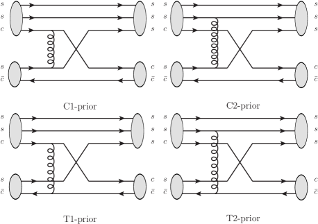
To get the transition amplitudes within the quark-interchange model, we take the same convention as the previous work Wang:2019spc ; Xiao:2019spy ; Wang:2020prk . The transition amplitude for the process can be decomposed as four processes in the hadronic molecular picture, which are illustrated in Fig. 2.
 |
The Hamiltonian of the initial hidden-charm molecular pentaquark state can be written as Wang:2019spc
| (3.3) |
where and are the Hamiltonian of the free baryon A and meson B, and denotes the interaction between the baryon A and the meson B.
Furthermore, we define the color wave function , the flavor wave function , the spin wave function , and the momentum space wave function , respectively. Thus, the total wave function can be expressed as
| (3.4) |
In this work, we take the Gaussian functions to approximate the momentum space wave functions for the baryon, meson, and molecule. The more explicit forms of the relevant Gaussian function can be found in Ref. Wang:2019spc , and the oscillating parameters of the meson and baryon are estimated by fitting their mass spectrum in the Godfrey-Isgur model Godfrey:1985xj , which are listed in Table 6. For an -wave loosely bound state composed of two hadrons A and B, the oscillating parameter can be related to the mass of the molecular state , i.e., with Weinberg:1962hj ; Weinberg:1963zza ; Guo:2017jvc . And then, the -matrix represents the relevant effective potential in the quark-interchange diagrams, which can be factorized as
| (3.5) |
where with the subscripts color, flavor, spin, and space stand for the corresponding factors, and the calculation details of these factors are referred to in Ref. Wang:2019spc .
For the two-body strong decay widths of these discussed molecular candidates, they can be explicitly expressed as
| (3.6) |
In the above expression, , , and stand for the momentum of the final state, the mass of the molecular state, and the transition amplitude of the discussed process, respectively. Here, we want to emphasize that there exists a relation of the transition amplitude and the -matrix , i.e.,
| (3.7) |
where and are the energies of the final states C and D, respectively. Through the above preparation, we can calculate the two-body hidden-charm strong decay widths of these proposed molecular states.
III.2 Two-body hidden-charm strong decay widths of these proposed molecular states
In the above section, our results suggest that the -wave state with and the -wave state with can be regarded as the hidden-charm molecular pentaquark candidates with triple strangeness. Thus, we will study the two-body strong decay property of these possible hidden-charm molecular pentaquarks with triple strangeness, which provides valuable information to search for these proposed molecular candidates in experiment.
In this work, we focus on the two-body hidden-charm strong decay channels for these predicted hidden-charm molecular pentaquarks with triple strangeness. For the -wave molecular state with , it can decay into the and channels through the -wave interaction. For the -wave molecular state with , we only take into account the decay channel via the -wave coupling, while the channel is suppressed since it is a -wave decay Wang:2019spc .
In order to intuitively clarify the uncertainty of the binding energies, we present the binding energies dependence of the decay widths for the -wave molecular state with and the -wave molecular state with in Fig. 3. As stressed in Sec. II, the hadronic molecule is a loosely bound state Chen:2017xat , so the binding energies of these hidden-charm molecular pentaquarks with triple strangeness change from to MeV in calculating the decay widths. With increasing the absolute values of the binding energy, the decay widths become larger, which is consistent with other theoretical calculations Chen:2017xat ; Lin:2017mtz ; Lin:2018kcc ; Lin:2018nqd ; Shen:2019evi ; Lin:2019qiv ; Lin:2019tex ; Dong:2019ofp ; Dong:2020rgs ; Xiao:2019mvs ; Wu:2018xaa ; Chen:2017abq ; Xiao:2016mho .
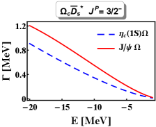
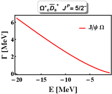
As illustrated in Fig. 3, when the binding energies are taken as MeV with typical values, the dominant decay channel is the around one MeV for the -wave molecular state with , and the decay width of the channel is predicted to be around several MeV for the -wave molecule with . Thus, the should be the promising channel to observe the -wave molecular state with and the -wave molecular state with . Meanwhile, it is interesting to note that the -wave molecular state with prefers to decay into the channel, but the decay width of the channel is comparable to the channel, which indicates that the -wave molecule with can be detected in the channel in future experiment.
In the heavy quark symmetry, the relative partial decay branch ratio between the and for the state with can be estimated as
| (3.8) |
since the relative momentum in the channel is larger than that in the channel, should be a little larger than , where is the binding energy. In our calculation, we obtain
Obviously, our results are consistent with the estimation in the heavy quark limit.
IV Summary
Searching for exotic hadronic state is an interesting and important research topic of hadron physics. With accumulation of experimental data, the LHCb observed three narrow , , and in 2019 Aaij:2019vzc , and found the evidence of the as a hidden-charm pentaquark with strangeness Aaij:2020gdg . These progresses make us have reason to believe that there should exist a zoo of the hidden-charm molecular pentaquark. At present, the hidden-charm molecular pentaquark with triple strangeness is still missing, which inspires our interest in exploring how to find these intriguing hidden-charm molecular pentaquark states with triple strangeness.
Mass spectrum information is crucial to searching for them. In this work, we perform the dynamical calculation of the possible hidden-charm molecular pentaquark states with triple strangeness from the interactions, where the effective potentials can be obtained by the OBE model. By finding bound state solutions of these discussed systems, we find that the most promising hidden-charm molecular pentaquarks with triple strangeness are the -wave state with and the -wave state with . Besides mass spectrum study, we also discuss their two-body hidden-charm strong decay behaviors within the quark-interchange model. In concrete calculation, we mainly focus on the and decay modes for the predicted -wave molecule with and the decay channel for the predicted -wave molecule with .
In the following years, the LHCb Collaboration will collect more experimental data at Run III and upgrade the High-Luminosity-LHC Bediaga:2018lhg . Experimental searches for these predicted hidden-charm molecular pentaquarks with triple strangeness are an area full of opportunities and challenges in future experiments.
ACKNOWLEDGMENTS
We would like to thank Z. W. Liu, G. J. Wang, L. Y. Xiao, and S. Q. Luo for very helpful discussions. This work is supported by the China National Funds for Distinguished Young Scientists under Grant No. 11825503, National Key Research and Development Program of China under Contract No. 2020YFA0406400, the 111 Project under Grant No. B20063, and the National Natural Science Foundation of China under Grant No. 12047501. R. C. is supported by the National Postdoctoral Program for Innovative Talent.
Appendix A Relevant subpotentials
Through the standard strategy Wang:2020dya ; Wang:2019nwt ; Wang:2019aoc , we can derive the effective potentials in the coordinate space for these investigated systems, i.e.,
| (1.1) | |||||
| (1.2) | |||||
| (1.3) | |||||
| (1.4) | |||||
| (1.5) | |||||
| (1.6) | |||||
| (1.7) | |||||
| (1.8) | |||||
| (1.9) | |||||
Here, and . Additionally, we also define several variables, which include , , , and . The function can be defined as
| (1.11) |
Here, and . Variables are defined as GeV, GeV, GeV, GeV, GeV, and GeV.
In the above effective potentials, we also introduce several operators, i.e.,
| (1.12) |
Here, is the tensor force operator. In Table 7, we collect the numerical matrix elements with the - wave mixing effect analysis. Of course, the relevant numerical matrix elements will be involved in the coupled channel analysis. For the coupled channel analysis with , we have , , , and . And, there exists , , , and for the coupled channel analysis with .
| Matrix elements | |||
|---|---|---|---|
| diag(1,1) | |||
| diag(1,1) | diag(1,1,1) | ||
| diag(,) | diag(,,) | ||
| diag(1,1,1) | diag(1,1,1,1) | diag(1,1,1,1) | |
| diag(,,) | diag(,,,) | diag(,,,) | |
References
- (1) S. K. Choi et al. (Belle Collaboration), Observation of a Narrow Charmonium-Like State in Exclusive Decays, Phys. Rev. Lett. 91, 262001 (2003).
- (2) H. X. Chen, W. Chen, X. Liu, and S. L. Zhu, The hidden-charm pentaquark and tetraquark states, Phys. Rep. 639, 1 (2016).
- (3) Y. R. Liu, H. X. Chen, W. Chen, X. Liu, and S. L. Zhu, Pentaquark and tetraquark states, Prog. Part. Nucl. Phys. 107, 237 (2019).
- (4) S. L. Olsen, T. Skwarnicki, and D. Zieminska, Nonstandard heavy mesons and baryons: Experimental evidence, Rev. Mod. Phys. 90, 015003 (2018).
- (5) F. K. Guo, C. Hanhart, U. G. Meiner, Q. Wang, Q. Zhao, and B. S. Zou, Hadronic molecules, Rev. Mod. Phys. 90, 015004 (2018).
- (6) X. Liu, An overview of new particles, Chin. Sci. Bull. 59, 3815 (2014).
- (7) A. Hosaka, T. Iijima, K. Miyabayashi, Y. Sakai, and S. Yasui, Exotic hadrons with heavy flavors: , , , and related states, Prog. Theor. Exp. Phys. 2016, 062C01 (2016).
- (8) N. Brambilla, S. Eidelman, C. Hanhart, A. Nefediev, C. P. Shen, C. E. Thomas, A. Vairo, and C. Z. Yuan, The states: Experimental and theoretical status and perspectives, Phys. Rep. 873, 1 (2020).
- (9) M. Gell-Mann, A schematic model of baryons and mesons, Phys. Lett. 8, 214 (1964).
- (10) G. Zweig, An SU(3) model for strong interaction symmetry and its breaking. Version 1, CERN, Report No. CERN-TH-401, 1964.
- (11) J. J. Wu, R. Molina, E. Oset, and B. S. Zou, Prediction of Narrow and Resonances with Hidden Charm Above 4 GeV, Phys. Rev. Lett. 105, 232001 (2010).
- (12) W. L. Wang, F. Huang, Z. Y. Zhang, and B. S. Zou, and states in a chiral quark model, Phys. Rev. C 84, 015203 (2011).
- (13) Z. C. Yang, Z. F. Sun, J. He, X. Liu, and S. L. Zhu, The possible hidden-charm molecular baryons composed of anticharmed meson and charmed baryon, Chin. Phys. C 36, 6 (2012).
- (14) J. J. Wu, T.-S. H. Lee, and B. S. Zou, Nucleon resonances with hidden charm in coupled-channel Models, Phys. Rev. C 85, 044002 (2012).
- (15) X. Q. Li and X. Liu, A possible global group structure for exotic states, Eur. Phys. J. C 74, 3198 (2014).
- (16) R. Chen, X. Liu, X. Q. Li, and S. L. Zhu, Identifying Exotic Hidden-Charm Pentaquarks, Phys. Rev. Lett. 115, 132002 (2015).
- (17) M. Karliner and J. L. Rosner, New Exotic Meson and Baryon Resonances from Doubly-Heavy Hadronic Molecules, Phys. Rev. Lett. 115, 122001 (2015).
- (18) R. Aaij et al. (LHCb Collaboration), Observation of Resonances Consistent with Pentaquark States in Decays, Phys. Rev. Lett. 115, 072001 (2015).
- (19) R. Aaij et al. (LHCb Collaboration), Observation of a Narrow Pentaquark State, , and of Two-Peak Structure of the , Phys. Rev. Lett. 122, 222001 (2019).
- (20) R. Aaij et al. (LHCb Collaboration), Evidence of a structure and observation of excited states in the decay, arXiv:2012.10380.
- (21) J. Hofmann and M. F. M. Lutz, Coupled-channel study of crypto-exotic baryons with charm, Nucl. Phys. A 763, 90 (2005).
- (22) J. J. Wu, R. Molina, E. Oset and B. S. Zou, Dynamically generated and resonances in the hidden charm sector around 4.3 GeV, Phys. Rev. C 84, 015202 (2011).
- (23) V. V. Anisovich, M. A. Matveev, J. Nyiri, A. V. Sarantsev, and A. N. Semenova, Nonstrange and strange pentaquarks with hidden charm, Int. J. Mod. Phys. A 30, 1550190 (2015).
- (24) Z. G. Wang, Analysis of the pentaquark states in the diquark-diquark-antiquark model with QCD sum rules, Eur. Phys. J. C 76, 142 (2016).
- (25) A. Feijoo, V. K. Magas, A. Ramos, and E. Oset, A hidden-charm pentaquark from the decay of into states, Eur. Phys. J. C 76, no. 8, 446 (2016).
- (26) J. X. Lu, E. Wang, J. J. Xie, L. S. Geng, and E. Oset, The reaction and a hidden-charm pentaquark state with strangeness, Phys. Rev. D 93, 094009 (2016).
- (27) H. X. Chen, L. S. Geng, W. H. Liang, E. Oset, E. Wang, and J. J. Xie, Looking for a hidden-charm pentaquark state with strangeness from decay into , Phys. Rev. C 93, 065203 (2016).
- (28) R. Chen, J. He, and X. Liu, Possible strange hidden-charm pentaquarks from and interactions, Chin. Phys. C 41, 103105 (2017).
- (29) C. W. Xiao, J. Nieves, and E. Oset, Prediction of hidden charm strange molecular baryon states with heavy quark spin symmetry, Phys. Lett. B 799, 135051 (2019).
- (30) C. W. Shen, H. J. Jing, F. K. Guo, and J. J. Wu, Exploring possible triangle singularities in the decay, Symmetry 12, 1611 (2020).
- (31) B. Wang, L. Meng, and S. L. Zhu, Spectrum of the strange hidden charm molecular pentaquarks in chiral effective field theory, Phys. Rev. D 101, 034018 (2020).
- (32) Q. Zhang, B. R. He, and J. L. Ping, Pentaquarks with the configuration in the Chiral Quark Model, arXiv:2006.01042.
- (33) H. X. Chen, W. Chen, X. Liu, and X. H. Liu, Establishing the first hidden-charm pentaquark with strangeness, arXiv:2011.01079.
- (34) F. Z. Peng, M. J. Yan, M. Sánchez Sánchez, and M. P. Valderrama, The pentaquark from a combined effective field theory and phenomenological perspectives, arXiv:2011.01915.
- (35) R. Chen, Can the newly be a strange hidden-charm molecular pentaquarks?, arXiv:2011.07214.
- (36) H. X. Chen, Hidden-charm pentaquark states through the current algebra: From their productions to decays, arXiv:2011.07187.
- (37) M. Z. Liu, Y. W. Pan, and L. S. Geng, Can discovery of hidden charm strange pentaquark states help determine the spins of and ?, Phys. Rev. D 103, 034003 (2021).
- (38) X. K. Dong, F. K. Guo, and B. S. Zou, A survey of heavy-antiheavy hadronic molecules, arXiv:2101.01021.
- (39) F. L. Wang, R. Chen, and X. Liu, Prediction of hidden-charm pentaquarks with double strangeness, Phys. Rev. D 103, 034014 (2021).
- (40) F. L. Wang, R. Chen, Z. W. Liu, and X. Liu, Probing new types of states inspired by the interaction between -wave charmed baryon and anti-charmed meson in a doublet, Phys. Rev. C 101, 025201 (2020).
- (41) T. Barnes and E. S. Swanson, A Diagrammatic approach to meson meson scattering in the nonrelativistic quark potential model, Phys. Rev. D 46, 131 (1992).
- (42) T. Barnes, N. Black, D. J. Dean, and E. S. Swanson, BB intermeson potentials in the quark model, Phys. Rev. C 60, 045202 (1999).
- (43) T. Barnes, N. Black, and E. S. Swanson, Meson meson scattering in the quark model: Spin dependence and exotic channels, Phys. Rev. C 63, 025204 (2001).
- (44) J. P. Hilbert, N. Black, T. Barnes, and E. S. Swanson, Charmonium-nucleon dissociation cross sections in the quark model, Phys. Rev. C 75, 064907 (2007).
- (45) G. J. Wang, X. H. Liu, L. Ma, X. Liu, X. L. Chen, W. Z. Deng, and S. L. Zhu, The strong decay patterns of and states in the relativized quark model, Eur. Phys. J. C 79, 567 (2019).
- (46) G. J. Wang, L. Y. Xiao, R. Chen, X. H. Liu, X. Liu, and S. L. Zhu, Probing hidden-charm decay properties of states in a molecular scenario, Phys. Rev. D 102, 036012 (2020).
- (47) L. Y. Xiao, G. J. Wang, and S. L. Zhu, Hidden-charm strong decays of the states, Phys. Rev. D 101, 054001 (2020).
- (48) G. J. Wang, L. Meng, L. Y. Xiao, M. Oka, and S. L. Zhu, Mass spectrum and strong decays of tetraquark states, arXiv:2010.09395.
- (49) R. Aaij et al. (LHCb Collaboration), Physics case for an LHCb Upgrade II-Opportunities in flavour physics, and beyond, in the HL-LHC era, arXiv:1808.08865.
- (50) M. B. Wise, Chiral perturbation theory for hadrons containing a heavy quark, Phys. Rev. D 45, R2188 (1992).
- (51) R. Chen, A. Hosaka, and X. Liu, Searching for possible -like molecular states from meson-baryon interaction, Phys. Rev. D 97, 036016 (2018).
- (52) G. J. Ding, Are and (4250) or hadronic molecules? Phys. Rev. D 79, 014001 (2009).
- (53) R. Casalbuoni, A. Deandrea, N. Di Bartolomeo, R. Gatto, F. Feruglio, and G. Nardulli, Light vector resonances in the effective chiral Lagrangian for heavy mesons, Phys. Lett. B 292, 371 (1992).
- (54) R. Casalbuoni, A. Deandrea, N. Di Bartolomeo, R. Gatto, F. Feruglio, and G. Nardulli, Phenomenology of heavy meson chiral Lagrangians, Phys. Rep. 281, 145 (1997).
- (55) T. M. Yan, H. Y. Cheng, C. Y. Cheung, G. L. Lin, Y. C. Lin, and H. L. Yu, Heavy quark symmetry and chiral dynamics, Phys. Rev. D 46, 1148 (1992); [Phys. Rev. D 55, 5851E (1997)].
- (56) M. Bando, T. Kugo, and K. Yamawaki, Nonlinear realization and hidden local symmetries, Phys. Rep. 164, 217 (1988).
- (57) M. Harada and K. Yamawaki, Hidden local symmetry at loop: A new perspective of composite gauge boson and chiral phase transition, Phys. Rep. 381, 1 (2003).
- (58) D. O. Riska and G. E. Brown, Nucleon resonance transition couplings to vector mesons, Nucl. Phys. A 679, 577 (2001).
- (59) R. Chen, Z. F. Sun, X. Liu, and S. L. Zhu, Strong LHCb evidence supporting the existence of the hidden-charm molecular pentaquarks, Phys. Rev. D 100, 011502 (2019).
- (60) J. He, Study of , , and in a quasipotential Bethe-Salpeter equation approach, Eur. Phys. J. C 79, 393 (2019).
- (61) J. He, and interactions and the LHCb hidden-charmed pentaquarks, Phys. Lett. B 753, 547 (2016).
- (62) R. Chen, F. L. Wang, A. Hosaka, and X. Liu, Exotic triple-charm deuteronlike hexaquarks, Phys. Rev. D 97, 114011 (2018).
- (63) F. L. Wang, R. Chen, Z. W. Liu, and X. Liu, Possible triple-charm molecular pentaquarks from interactions, Phys. Rev. D 99, 054021 (2019).
- (64) F. L. Wang and X. Liu, Exotic double-charm molecular states with hidden or open strangeness and around GeV, Phys. Rev. D 102, 094006 (2020).
- (65) G. Breit, The effect of retardation on the interaction of two electrons, Phys. Rev. 34, 553 (1929).
- (66) G. Breit, The fine structure of HE as a test of the spin interactions of two electrons, Phys. Rev. 36, 383 (1930).
- (67) N. A. Tornqvist, From the deuteron to deusons, an analysis of deuteronlike meson-meson bound states, Z. Phys. C 61, 525 (1994).
- (68) N. A. Tornqvist, On deusons or deuteron-like meson-meson bound states, Nuovo Cimento Soc. Ital. Fis. 107A, 2471 (1994).
- (69) P. A. Zyla et al. (Particle Data Group), Review of particle physics, PTEP 2020, no.8, 083C01 (2020).
- (70) R. Chen, A. Hosaka, and X. Liu, Prediction of triple-charm molecular pentaquarks, Phys. Rev. D 96, 114030 (2017).
- (71) C. Y. Wong, E. S. Swanson, and T. Barnes, Heavy quarkonium dissociation cross-sections in relativistic heavy ion collisions, Phys. Rev. C 65, 014903 (2002) Erratum: [Phys. Rev. C 66, 029901 (2002)].
- (72) S. Godfrey and N. Isgur, Mesons in a relativized quark model with chromodynamics, Phys. Rev. D 32, 189 (1985).
- (73) S. Weinberg, Elementary particle theory of composite particles, Phys. Rev. 130, 776 (1963).
- (74) S. Weinberg, Quasiparticles and the Born series, Phys. Rev. 131, 440 (1963).
- (75) Y. H. Lin, C. W. Shen, F. K. Guo, and B. S. Zou, Decay behaviors of the hadronic molecules, Phys. Rev. D 95, 114017 (2017).
- (76) Y. H. Lin, C. W. Shen, and B. S. Zou, Decay behavior of the strange and beauty partners of hadronic molecules, Nucl. Phys. A980, 21-31 (2018).
- (77) Y. H. Lin and B. S. Zou, Hadronic molecular assignment for the newly observed state, Phys. Rev. D 98, 056013 (2018).
- (78) C. W. Shen, J. J. Wu, and B. S. Zou, Decay behaviors of possible states in hadronic molecule pictures, Phys. Rev. D 100, 056006 (2019).
- (79) Y. H. Lin and B. S. Zou, Strong decays of the latest LHCb pentaquark candidates in hadronic molecule pictures, Phys. Rev. D 100, 056005 (2019).
- (80) Y. H. Lin, F. Wang, and B. S. Zou, Reanalysis of the newly observed state in a hadronic molecule model, Phys. Rev. D 102, 074025 (2020).
- (81) X. K. Dong, Y. H. Lin, and B. S. Zou, Prediction of an exotic state around 4240 MeV with as -parity partner of in molecular picture, Phys. Rev. D 101, 076003 (2020).
- (82) X. K. Dong and B. S. Zou, Prediction of possible bound states, arXiv:2009.11619.
- (83) D. Y. Chen, C. J. Xiao, and J. He, Hidden-charm decays of in a hadronic molecular scenario, Phys. Rev. D 96, 054017 (2017).
- (84) C. J. Xiao and D. Y. Chen, Possible hadronic molecule state, Eur. Phys. J. A 53, 127 (2017).
- (85) C. J. Xiao, Y. Huang, Y. B. Dong, L. S. Geng, and D. Y. Chen, Exploring the molecular scenario of , , and , Phys. Rev. D 100, 014022 (2019).
- (86) Q. Wu, D. Y. Chen, and F. K. Guo, Production of the states from the decays, Phys. Rev. D 99, 034022 (2019).