Hierarchical Clustering for Smart Meter Electricity Loads based on Quantile Autocovariances

Let’s assume that we observe $N$ time series, $\{\boldsymbol{X}_{1},\boldsymbol{X}_{2},\dots,\boldsymbol{X}_{N}\}$ where $\boldsymbol{X}_{i}=(X_{i,t_{i}},X_{i,t_{i}+1},\dots,X_{i,T_{i}})$ and $(t_{i},T_{i})$ denotes the first and the last times where the $i$-th time series is observed, respectively. In our dataset, the $(t_{i},T_{i})$ are the same for all time series but our procedures do not require this condition since they are based on extracted features from the time series. As mentioned in the previous section, there are many interesting features to consider as “clustering” variables instead of using raw data. In our case, we consider three sets of features that capture different aspects of the time series dynamic behaviour:

• •

  The set of autocorrelation coefficients of orders $(1,2,\dots,K)$, that is, we calculate the correlation coefficient between the variables $X_{i,t}$ and $X_{i,t+j}$ for $j=1,2,\dots,K$ defined by

  $$\rho_{i}(t,t+j)=\frac{Cov\left(X_{i,t},X_{i,t+j}\right)}{(Var(X_{i,t})Var(X_{i,t+j}))^{1/2}}.$$

  (1)

• •

  The set of partial autocorrelation coefficients of orders $(1,2,\dots,K)$, that is, we calculate the correlation coefficient between observations separated by $j$ periods, $X_{i,t}$ and $X_{i,t+j}$, when we eliminate the linear dependence due to intermediate values. The partial autocorrelation coefficient will be denoted by $\pi_{i}(t,t+j)$.

• •

  The set of quantile autocovariances of order $j$ at quantile levels $(\tau,\tau^{\prime})\in[0,1]^{2}$ defined by

  $\displaystyle\gamma_{i,(\tau,\tau^{\prime})}(t,t+j)=Cov\left(I(X_{i,t}\leq q_{\tau,i}),I(X_{i,t+j}\leq q_{\tau^{\prime},i})\right),$

  (2)

  where $I(\cdot)$ denotes the indicator function and $q_{\tau,i}$ and $q_{\tau^{\prime},i}$ are the $\tau-$ and $\tau^{\prime}-$quantiles of $X_{i,t}$ and $X_{i,t+j}$, respectively.

It is interesting to realize the differences among features (1) and (2) since both involve the calculation of a covariance between observations separated by $j$ periods. In (1), the covariance term is estimated by

$\displaystyle\frac{1}{T_{i}-j}\sum_{t=t_{i}}^{T_{i}-j}X_{i,t}X_{i,t+j}-\ \frac{1}{T_{i}-j}\sum_{t=t_{i}}^{T_{i}-j}X_{i,t}*\frac{1}{T_{i}-j}\sum_{t=t_{i}}^{T_{i}-j}X_{i,t+j},$

which involves the products $X_{i,t}X_{i,t+j}$ that can be distorted by extreme or outlier observations. For example, two very high loads observed at a distance of $j$ periods would spuriously increase the correlation at the $j-$lag. On the other hand, the quantile autocovariance (2) is estimated by

$\displaystyle\widehat{\gamma}_{i,(\tau,\tau^{\prime})}(t,t+j)=\frac{1}{T_{i}-j}\sum_{t=t_{i}}^{T_{i}-j}I(X_{i,t}\leq\widehat{q}_{\tau,i})I(X_{i,t+j}\leq\widehat{q}_{\tau^{\prime},i})\ -\ \tau\tau^{\prime}.$

(3)

The involved products $I(X_{i,t}\leq\widehat{q}_{\tau,i})I(X_{i,t+j}\leq\widehat{q}_{\tau^{\prime},i}$ are bounded which imply a negligible effect of outliers. The expression (3) can be interpreted as a mean of the number of times that values at $t$ below $\widehat{q}_{\tau,i}$ coincide with values at $t+j$ below $\widehat{q}_{\tau^{\prime},i}$. The term $\tau\tau^{\prime}$ is the number of coincidences that occur completely randomly. Therefore, a positive $\widehat{\gamma}_{i,(\tau,\tau^{\prime})}$ means that the number of matches is greater (smaller) than expected by chance.

It should be noticed that the above characteristics, in general, depend on $t$ and $j$, but if the time series are stationary, then they do not depend on $t$, which simplifies their analysis. For this reason, we consider the (daily) seasonal difference of the smart meter load (logarithmic transformed) time series. That is, as the time series that will be used in this paper present an half-hourly frequency, then $X_{i,t}=\ell_{i,t}-\ell_{i,t-48}$ are the series to be clustered, where $\ell_{i,t}=\log L_{i,t}$ denotes the logarithm of the load time series of the $i$-th smart meter. We should fix the largest lag, $K$, in the sets of autocorrelation and partial autocorrelation coefficients. We can fit autoregressive models to all the univariate time series, selecting the order by the BIC criterion, and take $K=\max_{1\leq i\leq N}(p_{i})$, where $p_{i}$ is the selected order for $i$-th time series. It is shown in [27] that this procedure provides an upper bound of the memory of $N$ stationary linear time series. The selected $K$ was 96. This selection allows us to captures the main linear dependencies in all time series. Also, for the set of quantile autocovariances, we should fix the lag and quantile levels. In this case, following the suggestions of [26], we use $j=1$ and $\tau\in\{0.1,0.5,0.9\}$ since these values have shown that they are capable of capturing and differentiating different types of nonlinearities. Finally, the three clustering analyzes will be based on the following sets of features:

1. a)

   $\boldsymbol{\rho}_{i}=\{\rho_{i}(1),\rho_{i}(2),\dots,\rho_{i}(96)\}_{i\in\{1,2,\dots,N\}}$

2. b)

   $\boldsymbol{\pi}_{i}=\{\pi_{i}(1),\pi_{i}(2),\dots,\pi_{i}(96)\}_{i\in\{1,2,\dots,N\}}$

3. c)

   $\boldsymbol{\gamma}_{i}=\{\gamma_{i},(0.1,0.1)$, $\gamma_{i},(0.1,0.5)$, $\gamma_{i},(0.1,0.9)$, $\gamma_{i}(0.5,0.1)$, $\gamma_{i}(0.5,0.5)$, $\gamma_{i}(0.5,0.9)$, $\gamma_{i}(0.9,0.1)$, $\gamma_{i}(0.9,0.5)$, $\gamma_{i}(0.9,0.9)\}_{i\in\{1,2,\dots,N\}}$

Thus, the analysis will be based on $96\times 1$ vectors of features for autocorrelation and partial autocorrelation coefficients and based on $9\times 1$ vectors of features for quantile autocovariances. Once we have the vectors of features, we define a dissimilarity measure between time series $\boldsymbol{X}_{i}$ and $\boldsymbol{X}_{j}$ by the Euclidean distance of the corresponding vectors. That is:

1. a)

   $d_{AC}(\boldsymbol{X}_{i},\boldsymbol{X}_{j})=\|\boldsymbol{\rho}_{i}-\boldsymbol{\rho}_{j}\|_{2}$

2. b)

   $d_{PAC}(\boldsymbol{X}_{i},\boldsymbol{X}_{j})=\|\boldsymbol{\pi}_{i}-\boldsymbol{\pi}_{j}\|_{2}$

3. c)

   $d_{QC}(\boldsymbol{X}_{i},\boldsymbol{X}_{j})=\|\boldsymbol{\gamma}_{i}-\boldsymbol{\gamma}_{j}\|_{2}$

where $\|\cdot\|$ denotes de Euclidean distance.

The distances $d_{M}(\boldsymbol{X}_{i},\boldsymbol{X}_{j})$ will be obtained for all pairs $(i,j)$ with $i\neq j$ to construct the following $N\times N$ dissimilarity matrix

$\displaystyle\boldsymbol{DM}_{M}=\begin{pmatrix}0&d_{M}(X_{1},X_{2})&\ldots&d_{M}(X_{1},X_{N})\\ d_{M}(X_{2},X_{1})&0&\ldots&d_{M}(X_{2},X_{N})\\ \vdots&\vdots&\ddots&\vdots\\ d_{M}(X_{N},X_{1})&d_{M}(X_{N},X_{2})&\ldots&0\end{pmatrix}$

(4)

where $M\in\{AC,PAC,QC\}$. The dissimilarity matrix (4) can be used in any cluster procedure which requires this kind of input. In particular, we can apply hierarchical clustering since it allows us to identify clusters as well as hierarchies among the clusters. In hierarchical cluster procedures, to decide which groups should be combined, it is necessary to choose a measure of dissimilarity (linkage criterion) between sets. It is important to emphasize that this choice will influence the shape of the groups, since some sets could be close according to one distance and far according to another. The three best known measures are minimum or single-linkage ($d_{s}$), maximum or complete-linkage ($d_{c}$) and average linkage ($d_{a}$) defined by:

$$d_{s}(A,B)=\min\{d(X_{i},X_{j}):i\in A,j\in B\}$$

$$d_{c}(A,B)=\max\{d(X_{i},X_{j}):i\in A,j\in B\}$$

$$d_{a}(A,B)=\frac{1}{n_{A}n_{B}}\sum_{i=1}^{n_{A}}\sum_{i=1}^{n_{B}}d(X_{i},X_{j}),$$

where $A$ and $B$ are two sets of observations having $n_{A}$ and $n_{B}$ elements, respectively.

In this work, we prefer to use complete linkage as it ensures that the observations in a group are “similar” to all observations of the same group in the sense that once the cut-off point in the dendrogram has been set all the distances within of a cluster are smaller than this cut-off point.

Once we obtain the groups, an interesting question is to know which variables have been the most relevant to form these groups. This question can be addressed through the use of a supervised classification procedure where the labels of the observations will be the result of the clustering methodology. That is, if we have $k$ clusters, we will assign the labels $\{1,2,\ldots,k\}$ to the observations of the respective clusters. These labels and the features will be the input of the supervised classification procedure. In this work, we will use decision trees [28] for multiclass classification problem since for this procedure unbiased estimates of the predictor (feature) importance [29] are available.

In this section we use the public energy consumption dataset from [30]. It includes a sample of 5,567 households of London with their individual electricity consumption time series during 2013, in kWh (per half hour), date and time, and CACI ACORN segmentation (6 geo-demographic categories) [31]. In particular, to validate this work’s clustering methodology, we will compare the resulting clusters with the geo-demographic aggregated categories coded as “ACORN_GROUPED”, which classify households into three main groups: “Affluent”, “Comfortable” and “Adversity”. Moreover, the dataset is also divided into two subgroups of consumers:

• i)

  std tariff: Consumers whose electricity tariff is fixed (standard) to a constant price during the time of the study.

• ii)

  tou tariff: Consumers with “time of use” tariff for which the electricity price is different for each hour.

In order to better characterized the inherent consumption behavior of individual households, we have focused the following study on the std tariff consumers, as these are not influenced by a variable price signal. This initial group includes approximately 4500 time series from which some of them are discarded, due a high proportion of missing observation, rendering a final subsample of around 3200 time series (households).

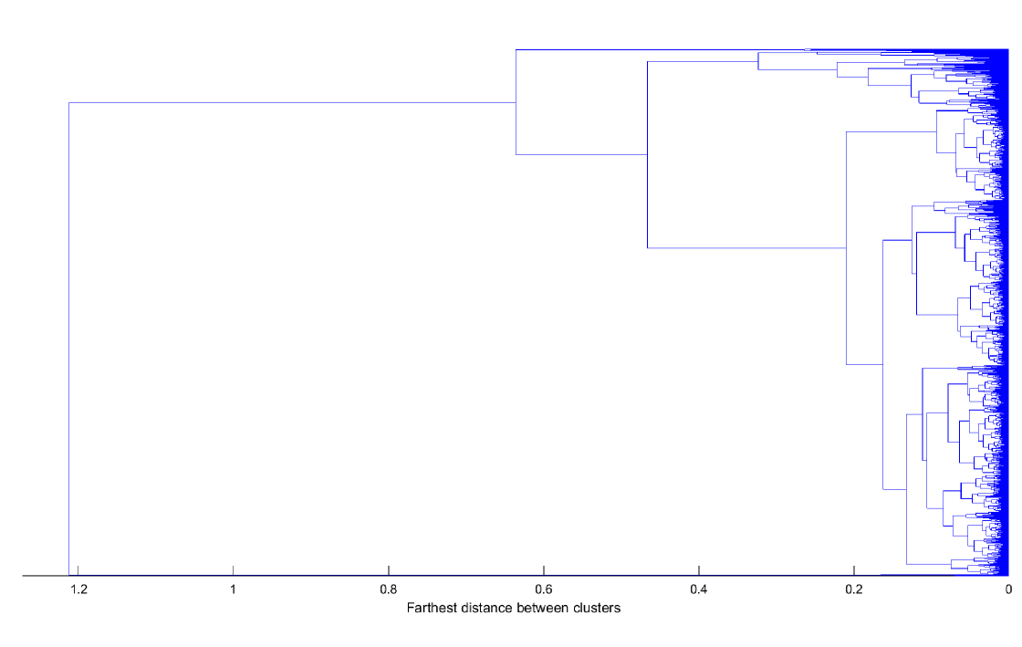
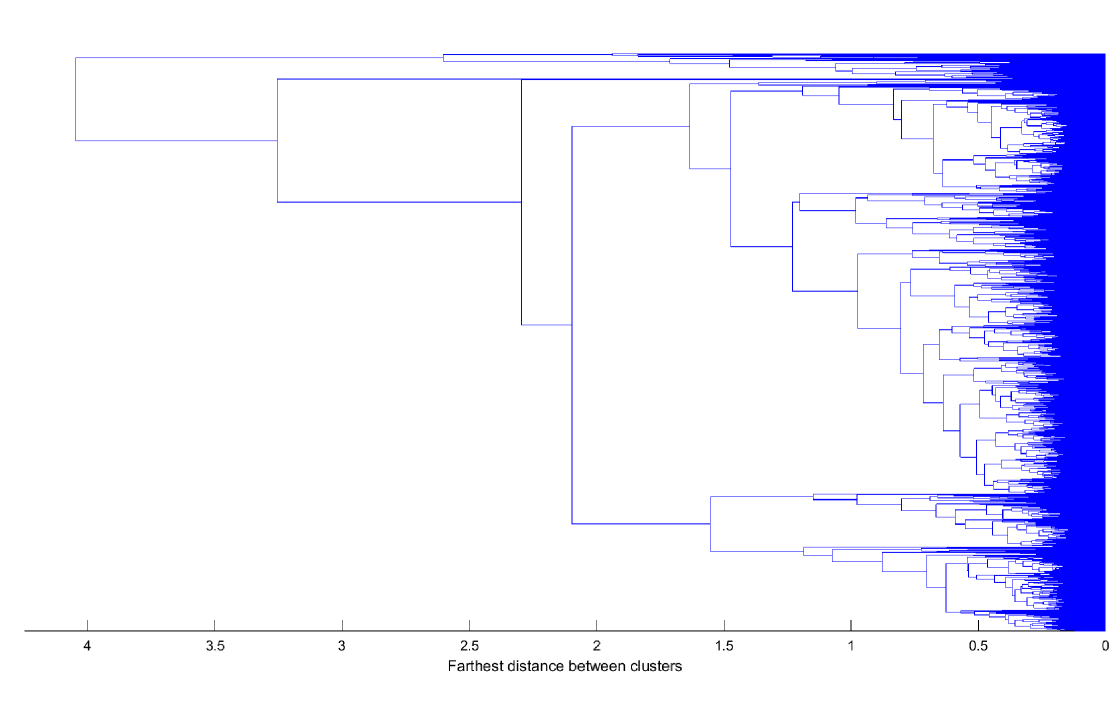
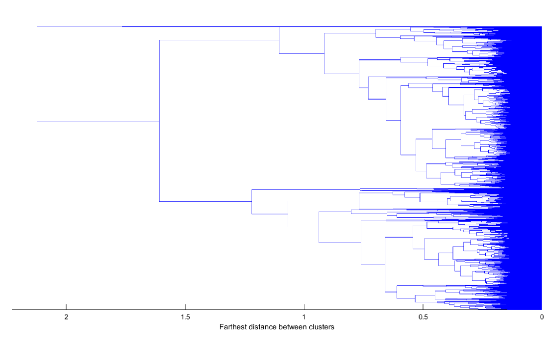
The following three dendrograms, Fig. 1 - 3, are obtained using the QC, AC and PAC features and complete linkage introduced in Section II. In the three graphs we can observe some clear groups of observations (time series) and also observations that are joined to the hierarchical structure at large levels. Those observations have a dynamic “atypical” behavior and are grouped in clusters with less than 1% of the total number of time series. Once we discard the atypical observations, we find eight, six and seven large clusters for QC, AC and PAC, respectively. Moreover, the degrees of coincidence among these three clusters partitions are low as indicated by the adjusted Rand indexes (0.0941 when comparing QC and AC; 0.1432 when comparing QC and PAC and 0.2687 when comparing AC and PAC). This implies that the three approaches look at different characteristics of the time series.

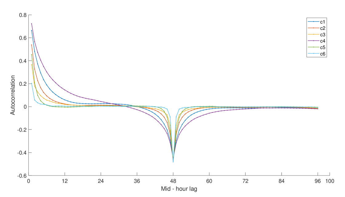
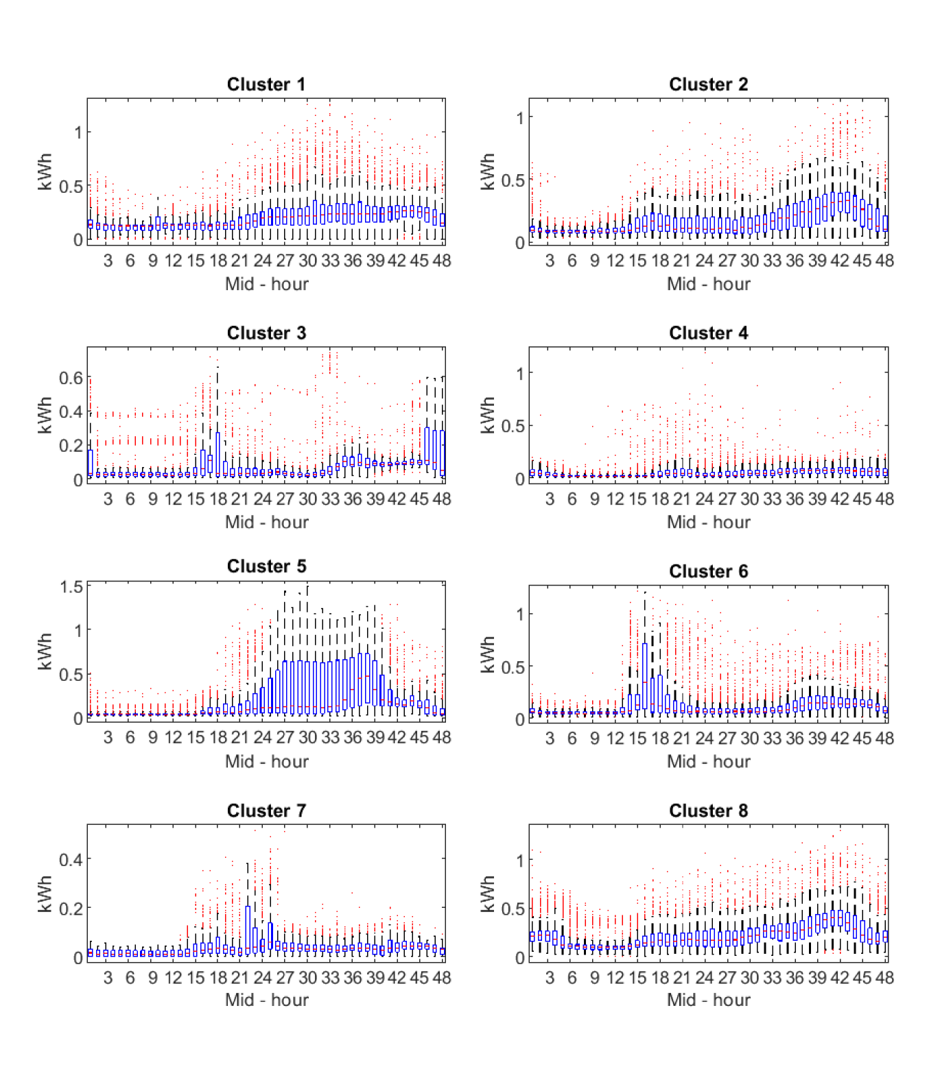
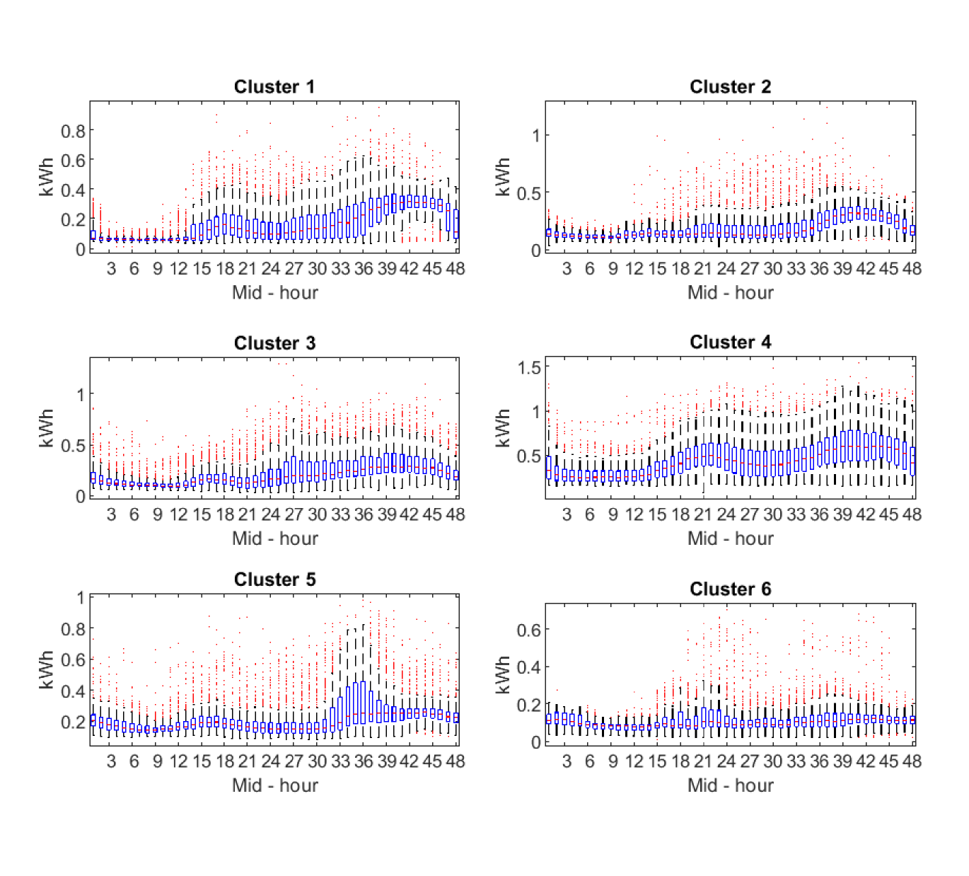
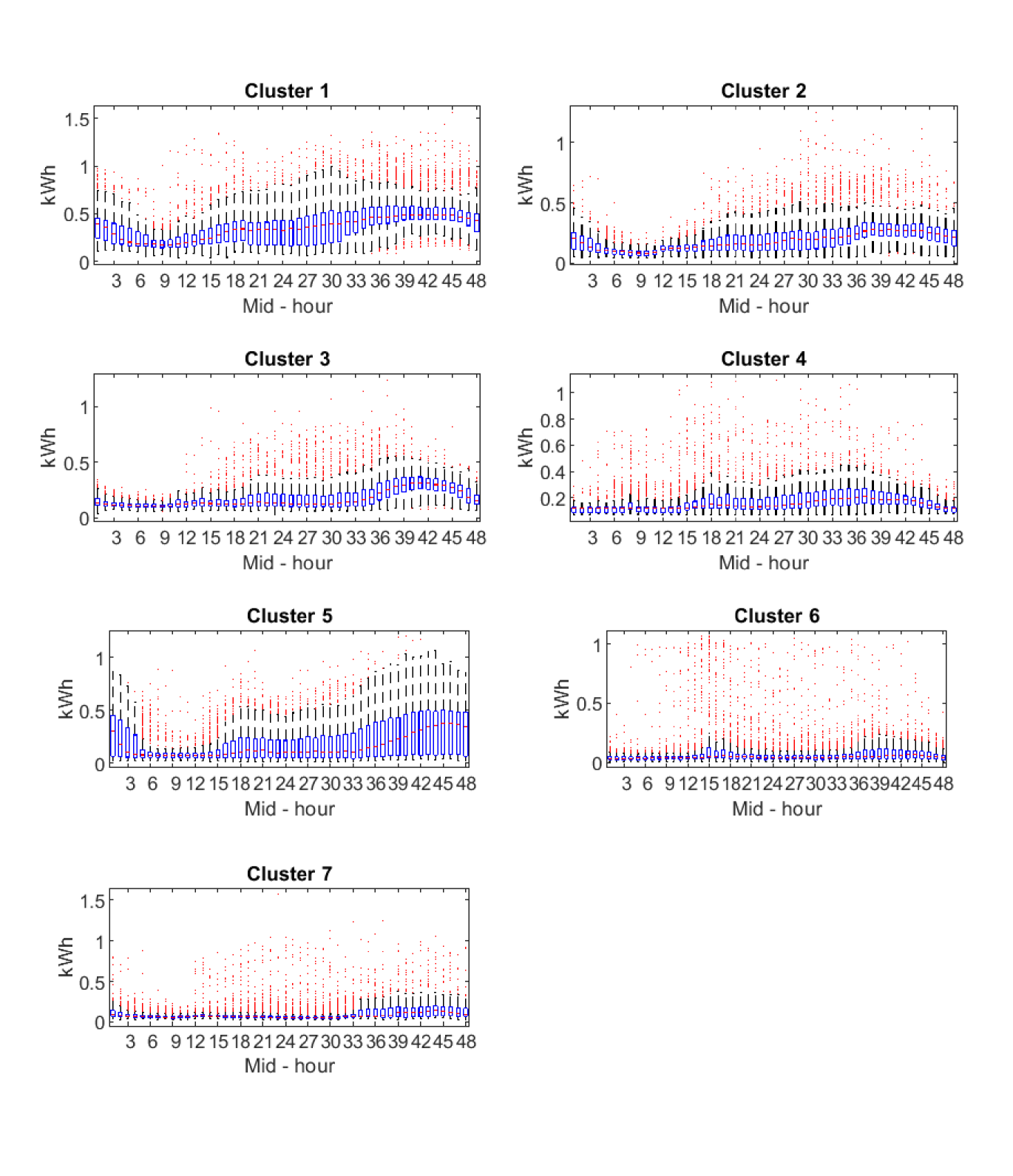
Figures 4 - 6 illustrate these large clusters obtained with QC, AC and PAC, respectively. In the figures, we represent the mean of the features used to obtain the clusters. There are nine features, in the case of QC, corresponding to the covariance of quantiles 10%, 50% and 90%. In the case of AC and PAC, we use the first 96 simple and partial autocorrelations, respectively. The clusters based on QC reveals differences in the median consumptions (.5 versus .5) and highest versus median consumptions (.9 versus .5). For instance, it is remarkable the difference between c3 and c7 versus c1, c2, c4, c6 and c8 at the median consumptions. The c3 and c7 have negative covariances and the c1, c2, c4, c6 and c8 have positive ones. That is, in the first group, a consumption below the median tends to be followed by consumption above the median, while the second group tends to maintain their consumption below the median. The groups by SAC and PAC show differences in the short range dependencies but also in the way they are around the lag 48 (one day). We can focus on the first correlations coefficients that show different degrees of persistency in the consumptions. For instance, in the AC clusters, there is a clear order from high dependency at c4, c1 and c2, medium at c3 and c5 and to low dependency at c6. At the PAC clusters, we can differentiate between clusters with negative second partial autocorrelation (c1, c2 and c6), medium (c3, c4, and c5) and hight positive (c7). That is, once we eliminate the first order correlation, there are negative (or positive) direct effects on the consumption at the 2-step ahead period.

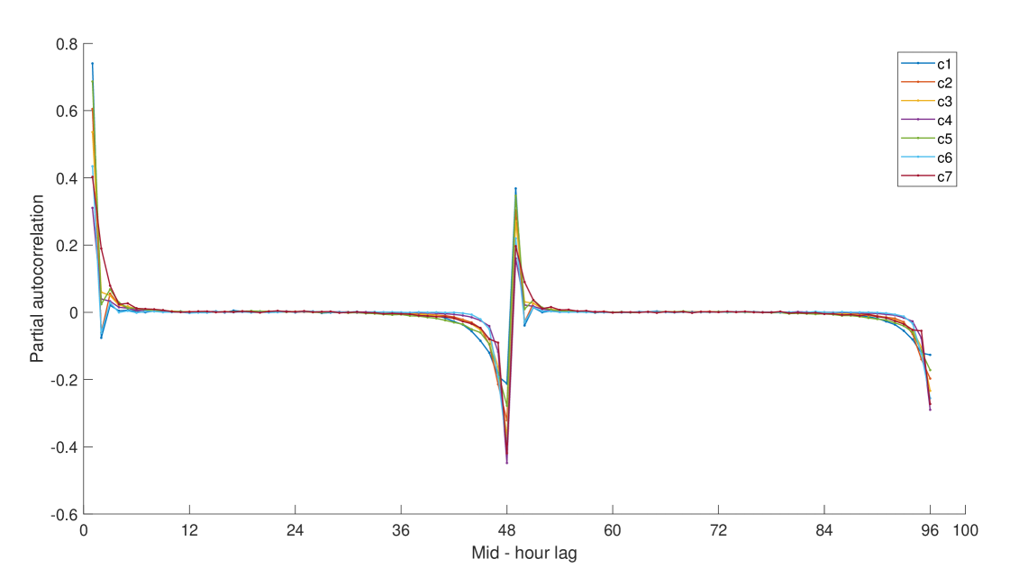
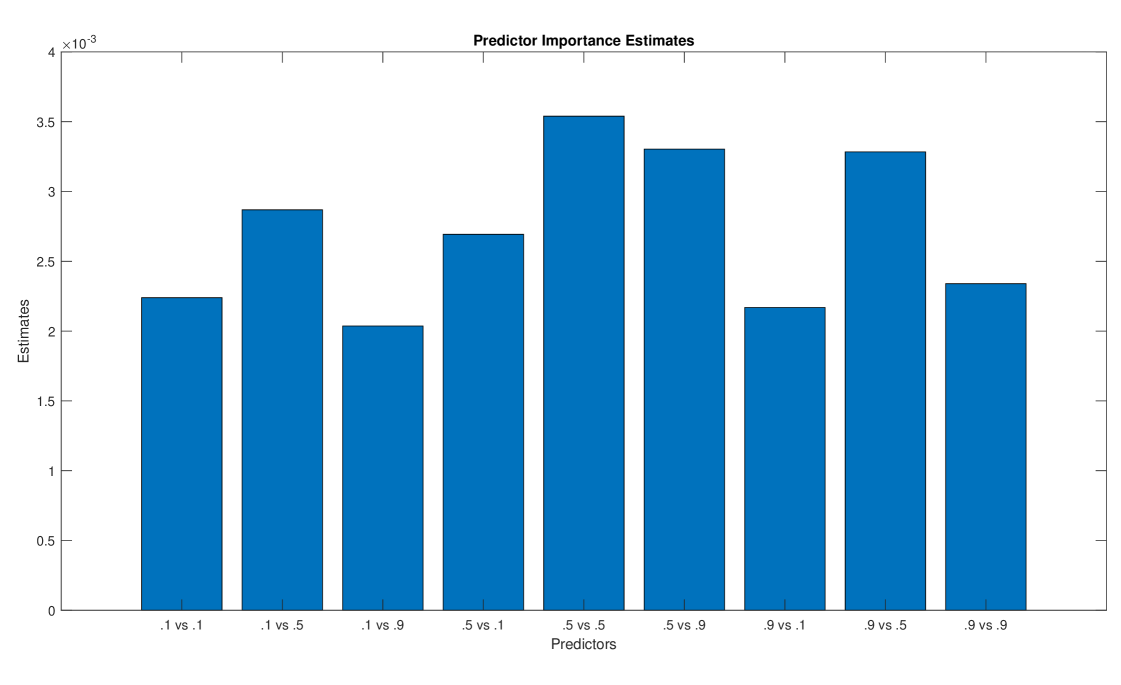
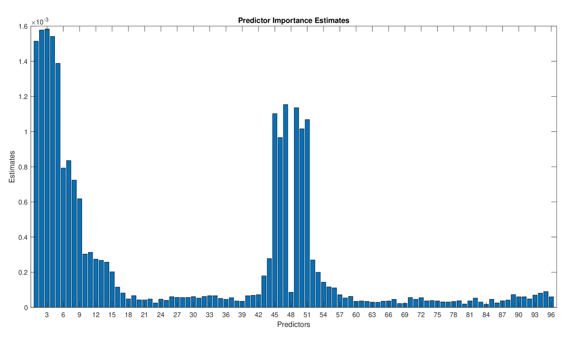
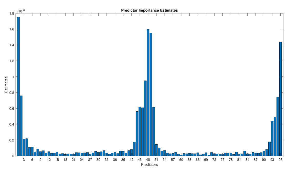
Figures 7 - 9 provide the estimates of the predictor importance. It is clear that all features are relevant in the clustering based on QC but we can make a selection of features in the clusterings based on SAC and PAC. In particular, for SAC, the first fifteen lags and the four lags around the 48–lag appear to be relevant and, for PAC, the first four lags and the four lags before and two lags after the 48– and 96–lags as well as those daily “seasonal” lags. It is interesting to notice that the 48–lag is not relevant in the SAC but this is due to the (daily) seasonal difference. However, there are still stationary seasonal behavior as reflected by relevant predictors/lags around the 48–lag. For PAC, the daily lags are highly relevant. The misclassification rates estimated by cross–validation for the three trained decision trees were 9.9%, 23.3% and 21.4% when using QC, SAC and PAC, respectively. These low rates point out that the obtained trees are good approximations to the clustering mechanism. Of course, other supervised classification procedures such as random forest or neural networks can be used in order to obtain better approximations.

Tables I - III show the number of households on each cluster that are classified in the three ACORN_GROUPED categories. Note that they are unevenly distributed across clusters. Indeed, we have performed chi-squared tests in those tables and the results are highly significant in the three cases revealing that clustering is related to ACORN_GROUPED classification. This shows that the proposed clustering methodology is able to, up to some representative extend, provide insights on the geo-demographic characteristics of a household (Acorn groups), just by studying the time series dependencies.

Figures 10 - 12 show the prototype’s hourly profile for each cluster. The prototype is the medoid of each cluster, that is, the element in the cluster with minimal average dissimilarity to all objects in the cluster. We can observe different characteristic consumption patterns associated to different types of consumers. For instance, the eight clusters obtained with quantile autocovariance and complete linkage in Figure 10 allow distinguishing between consumers with morning (clusters 3, 6 and 7) and evening (clusters 1, 2, 5 and 8) peak loads, and those with a more constant consumption pattern (cluster 4). This is also appreciated in the 6 clusters obtained with autocorrelation coefficients and complete linkage in Figure 11. In this case, clusters 1 and 4 capture those consumers with two intermediate peak loads in the morning and in the evening. Cluster 5 represents consumers with a single peak consumption in the afternoon, and clusters 2, 3 and 5, present consumers with less volatility.

Similarly, Figure 12 shows the clusters obtained with partial autocorrelation coefficients and complete linkage. Clusters 1, 2 and 5 characterize consumers with a steady increasing load that reach its maximum at midnight, while clusters 3, 4, 6 and 7, represent consumers with two intermediate peaks in the morning and evening. In this case clusters from each type are mainly differentiated by the average load consumption levels.

In this work we have presented three different hierarchical-based clustering strategies based on a set “dissimilarity” measures computed over: quantile auto-covariances, and simple and partial autocorrelations. The main advantage of this approach is that we can summarize each series in only a set of representative features which makes them very easy to implement (highly efficient), easy to automatize and scalable to hundreds of thousands of series, i.e., valid for real-world applications with large datasets of time series, as the ones obtained from smart meters. We evaluate the performance of these clustering models with thousands of electricity consumption time series. The results are promising: we are able to obtain highly representative clusters capturing different electricity load consumption patterns and identifying the level of influence of each of the models’ features. Moreover, we have seen how the proposed clustering scheme can provide meaningful insights on the geo-demographic level of a household (Acorn groups), just by analyzing its time series dependencies (autocorrelations).

The authors gratefully acknowledge the financial support from the Spanish government through project MTM2017-88979-P and from Fundación Iberdrola through “Ayudas a la Investigación en Energía y Medio Ambiente 2018”.

References

- [1] R. Hierzinger, M. Albu, H. Van Elburg, A. J. Scott, A. Łazicki, L. Penttinen, F. Puente, and H. Sæle, “European smart metering landscape report 2012,” SmartRegions Deliverable, vol. 2, 2012.
- [2] S. S. S. R. Depuru, L. Wang, V. Devabhaktuni, and N. Gudi, “Smart meters for power grid—challenges, issues, advantages and status,” in 2011 IEEE/PES Power Systems Conference and Exposition. IEEE, 2011, pp. 1–7.
- [3] B. Yildiz, J. Bilbao, J. Dore, and A. Sproul, “Recent advances in the analysis of residential electricity consumption and applications of smart meter data,” Applied Energy, vol. 208, pp. 402–427, 2017.
- [4] Y. Wang, Q. Chen, T. Hong, and C. Kang, “Review of smart meter data analytics: Applications, methodologies, and challenges,” IEEE Transactions on Smart Grid, vol. 10, no. 3, pp. 3125–3148, 2018.
- [5] A. Al-Wakeel, J. Wu, and N. Jenkins, “K-means based load estimation of domestic smart meter measurements,” Applied energy, vol. 194, pp. 333–342, 2017.
- [6] G. Chicco, “Overview and performance assessment of the clustering methods for electrical load pattern grouping,” Energy, vol. 42, no. 1, pp. 68–80, 2012.
- [7] M. Koivisto, P. Heine, I. Mellin, and M. Lehtonen, “Clustering of connection points and load modeling in distribution systems,” IEEE Transactions on Power Systems, vol. 28, no. 2, pp. 1255–1265, 2012.
- [8] J. Kwac, J. Flora, and R. Rajagopal, “Household energy consumption segmentation using hourly data,” IEEE Transactions on Smart Grid, vol. 5, no. 1, pp. 420–430, 2014.
- [9] A. Lavin and D. Klabjan, “Clustering time-series energy data from smart meters,” Energy efficiency, vol. 8, no. 4, pp. 681–689, 2015.
- [10] F. McLoughlin, A. Duffy, and M. Conlon, “A clustering approach to domestic electricity load profile characterisation using smart metering data,” Applied energy, vol. 141, pp. 190–199, 2015.
- [11] A. Tureczek, P. Nielsen, and H. Madsen, “Electricity consumption clustering using smart meter data,” Energies, vol. 11, no. 4, p. 859, 2018.
- [12] Y. Wang, Q. Chen, C. Kang, and Q. Xia, “Clustering of electricity consumption behavior dynamics toward big data applications,” IEEE transactions on smart grid, vol. 7, no. 5, pp. 2437–2447, 2016.
- [13] C. Beckel, L. Sadamori, T. Staake, and S. Santini, “Revealing household characteristics from smart meter data,” Energy, vol. 78, pp. 397–410, 2014.
- [14] A. Kavousian, R. Rajagopal, and M. Fischer, “Determinants of residential electricity consumption: Using smart meter data to examine the effect of climate, building characteristics, appliance stock, and occupants’ behavior,” Energy, vol. 55, pp. 184–194, 2013.
- [15] J. P. Gouveia and J. Seixas, “Unraveling electricity consumption profiles in households through clusters: Combining smart meters and door-to-door surveys,” Energy and Buildings, vol. 116, pp. 666–676, 2016.
- [16] S. Haben, C. Singleton, and P. Grindrod, “Analysis and clustering of residential customers energy behavioral demand using smart meter data,” IEEE transactions on smart grid, vol. 7, no. 1, pp. 136–144, 2015.
- [17] B. Stephen, A. J. Mutanen, S. Galloway, G. Burt, and P. Järventausta, “Enhanced load profiling for residential network customers,” IEEE Transactions on Power Delivery, vol. 29, no. 1, pp. 88–96, 2013.
- [18] O. Y. Al-Jarrah, Y. Al-Hammadi, P. D. Yoo, and S. Muhaidat, “Multi-layered clustering for power consumption profiling in smart grids,” IEEE Access, vol. 5, pp. 18 459–18 468, 2017.
- [19] R. Al-Otaibi, N. Jin, T. Wilcox, and P. Flach, “Feature construction and calibration for clustering daily load curves from smart-meter data,” IEEE Transactions on industrial informatics, vol. 12, no. 2, pp. 645–654, 2016.
- [20] S. Zhong and K.-S. Tam, “Hierarchical classification of load profiles based on their characteristic attributes in frequency domain,” IEEE Transactions on Power Systems, vol. 30, no. 5, pp. 2434–2441, 2014.
- [21] R. Granell, C. J. Axon, and D. C. Wallom, “Impacts of raw data temporal resolution using selected clustering methods on residential electricity load profiles,” IEEE Transactions on Power Systems, vol. 30, no. 6, pp. 3217–3224, 2014.
- [22] K. Bandara, C. Bergmeir, and S. Smyl, “Forecasting across time series databases using recurrent neural networks on groups of similar series: A clustering approach,” arXiv preprint arXiv:1710.03222, 2017.
- [23] F. L. Quilumba, W.-J. Lee, H. Huang, D. Y. Wang, and R. L. Szabados, “Using smart meter data to improve the accuracy of intraday load forecasting considering customer behavior similarities,” IEEE Transactions on Smart Grid, vol. 6, no. 2, pp. 911–918, 2014.
- [24] M. Chaouch, “Clustering-based improvement of nonparametric functional time series forecasting: Application to intra-day household-level load curves,” IEEE Transactions on Smart Grid, vol. 5, no. 1, pp. 411–419, 2013.
- [25] B. Yildiz, J. I. Bilbao, J. Dore, and A. Sproul, “Household electricity load forecasting using historical smart meter data with clustering and classification techniques,” in 2018 IEEE Innovative Smart Grid Technologies-Asia (ISGT Asia). IEEE, 2018, pp. 873–879.
- [26] B. Lafuente-Rego and J. A. Vilar, “Clustering of time series using quantile autocovariances,” Advances in Data Analysis and classification, vol. 10, no. 3, pp. 391–415, 2016.
- [27] A. M. Alonso and D. Peña, “Clustering time series by linear dependency,” Statistics and Computing, vol. 29, no. 4, pp. 655–676, 2019.
- [28] L. Breiman, J. Friedman, C. Stone, and R. Olshen, Classification and Regression Trees, ser. The Wadsworth and Brooks-Cole statistics-probability series. Taylor & Francis, 1984.
- [29] H. Ishwaran, “Variable importance in binary regression trees and forests,” Electronic Journal of Statistics, vol. 1, pp. 519–537, 2007.
- [30] [Online]. Available: https://data.london.gov.uk/dataset/smartmeter-energy-use-data-in-london-households
- [31] [Online]. Available: https://acorn.caci.co.uk/downloads/Acorn-User-guide.pdf