table
Hierarchical models for small area estimation using zero-inflated forest inventory variables: comparison and implementation
Abstract
National Forest Inventory (NFI) data are typically limited to sparse networks of sample locations due to cost constraints. While traditional design-based estimators provide reliable forest parameter estimates for large areas, there is increasing interest in model-based small area estimation (SAE) methods to improve precision for smaller spatial, temporal, or biophysical domains. SAE methods can be broadly categorized into area- and unit-level models, with unit-level models offering greater flexibility—making them the focus of this study. Ensuring valid inference requires satisfying model distributional assumptions, which is particularly challenging for NFI variables that exhibit positive support and zero inflation, such as forest biomass, carbon, and volume. Here, we evaluate a class of two-stage unit-level hierarchical Bayesian models for estimating forest biomass at the county-level in Washington and Nevada, United States. We compare these models to simpler Bayesian single-stage and two-stage frequentist approaches. To assess estimator performance, we employ simulated populations and cross-validation techniques. Results indicate that small area estimators that incorporate a two-stage approach to account for zero inflation, county-specific random intercepts and residual variances, and spatial random effects provide the most reliable county-level estimates. Additionally, findings suggest that unit-level cross-validation within the training dataset is as effective as area-level validation using simulated populations for model selection. We also illustrate the usefulness of simulated populations for better assessing qualities of the various estimators considered.
Keywords: model-based, Gaussian process, spatial, Bayesian, carbon, biomass, simulation
1 Introduction
National Forest Inventories (NFIs) play a critical role in collecting data and monitoring forest trends to assess resource availability, health, composition, and other economic and ecological attributes across various spatial scales within a given country. In the United States, the NFI is conducted by the United States Department of Agriculture (USDA) Forest Service through the Forest Inventory and Analysis (FIA) Program. Traditionally, NFIs such as FIA have been designed to provide precise estimates at broader spatial scales, such as state-level assessments of forest attributes like timber volume and biomass. However, there is growing national interest, along with increased funding, in obtaining more precise biomass estimates at finer spatial scales, such as the county-level (Wiener et al.,, 2021; Prisley et al.,, 2021; U.S. Senate,, 2023). This rising demand, coupled with the widespread availability of high-resolution remote sensing data, has prompted researchers to develop and apply innovative small area estimation (SAE) methods that integrate FIA data with remote sensing products (Cao et al.,, 2022; May et al.,, 2023; Finley et al.,, 2024).
Despite the wide variety of SAE methods, they can generally be categorized into two main approaches: area-level and unit-level methods (Rao and Molina,, 2015). Both aim to estimate the same parameter of interest but differ significantly in their use of data. In area-level modeling, survey unit response variable measurements are aggregated at each area. These aggregates are referred to as direct estimates and are typically generated using a design-based estimator. Direct estimates are then set as the area-level response variable in a regression model that might include area-level summaries of predictor variables and structured random effects. The goal of areal models is to use sources of auxiliary information to smooth noisy direct estimates. In contrast, unit-level approaches retain response variable measurements at the individual unit level. Set as the response variable, these unit-level measurements are coupled with spatial and/or temporally aligned predictor variables, possibly along with structured random effects, in a predictive model. This predictive model is then used to predict for all unobserved units. Finally, predictions are aggregated to any user-defined area of interest.
The advantages and trade-offs of SAE approaches have only begun to be explored in the forest inventory literature. Area-level modeling often benefits from a more linear relationship between response and predictor variables and does not require precise plot locations, which is particularly useful given the often confidentiality of NFI plot data. However, aggregation leads to data loss, limits the ability to model fine-scale (i.e., unit-level) relationships, precludes delineation of new areas of interest after model fitting, and imposes statistical assumptions that might be difficult to justify. For example, in the classical Fay-Herriot model, within-area variance of the direct estimate is assumed to be fixed and known, although in practice it is estimated from limited data. These variances enter the area-level model through a random effect, often without strong theoretical justification or consistency between the two inferential paradigms. In contrast, unit-level approaches leverage precise plot locations to model fine-scale spatial relationships more effectively, making them particularly valuable when such data are available.
Unlike design-based estimators, which are determined by the sampling design, inference from model-based estimators relies entirely on the selection of an appropriate model. Consequently, we must take special care when specifying SAE models and conduct rigorous model checking. One of the most effective ways to assess SAE models is through simulated populations that closely resemble the true, but only partially observed, population of interest. Simulated populations allow us to explore how inference varies under different conditions (e.g., varying sample sizes) and to compare our estimates against “true” values. To ensure a meaningful evaluation, we must generate these simulated populations using methods that are not similar to the models we hope to assess.
Beyond assessment using simulated populations, we can evaluate models through cross-validation using observed data (e.g., leave-one-out or -fold cross-validation). However, in SAE studies, the primary parameters of interest exist at the area level. Unit-level models can be assessed using cross-validation at the unit level (i.e., iteratively holdout one or more observations, predict for those holdout, and compare the predictions to the holdout true values); however, such unit-level assessments might not reveal how well the estimator performs once predictions are aggregated to the desired areas of interest.
This study evaluates a range of unit-level SAE approaches for estimating average biomass at the county level in Washington and Nevada. A key challenge in this context arises when estimating biomass across areas with a mix of forest and non-forest landcover. Specifically, biomass values exhibit a mixture of continuous positive values and true zeroes, a phenomenon referred to here as “zero-inflation.” While the term zero-inflation is commonly used in the statistical literature to describe a discrete distribution with an excessive number of zeros, in this case, biomass follows a continuous distribution with an additional zero component. Various model-based approaches have been developed to address zero-inflation in SAE. Notably, Pfeffermann et al., (2008) introduced a two-stage mixture model to account for zero-inflation in the response variable, exploring both frequentist and Bayesian modes of inference. Their findings suggest that mean squared error (MSE) estimation is more straightforward in the Bayesian paradigm due to the advantages of Markov chain Monte Carlo (MCMC) simulation in uncertainty propagation across the model stages. Expanding on this work, Chandra and Sud, (2012) applied the same two-stage model in a frequentist setting and introduced a parametric bootstrap-based MSE estimator.
In forest inventory applications, zero-inflation has received relatively limited attention. Finley et al., (2011) developed a two-stage model for zero-inflation in continuous forest attributes such as biomass, volume, and age, employing a hierarchical Bayesian framework with Gaussian process-based spatial random effects. Their approach enables unit-level predictions of forest attributes along with uncertainty quantification, though they did not directly produce small area estimates. More recently, White et al., (2025) applied the zero-inflated SAE model from Chandra and Sud, (2012) to FIA data in Nevada, generating county-level biomass estimates. Their study compared the zero-inflated estimator to other commonly used small area estimators, including the Battese-Harter-Fuller unit-level model and the Fay-Herriot area-level model (Fay and Herriot,, 1979; Battese et al.,, 1988). Their simulation results indicate the zero-inflated model improves point estimates and produces competitive MSE estimates, though further refinements remain possible (see Figure 2 in White et al.,, 2025).
In this study, we compare and extend model-based SAE approaches that account for zero-inflation, applying them to FIA data and remote sensing products for Washington and Nevada, as described in Section 2.1. Specifically, we evaluate nine model-based approaches, including the zero-inflated estimator from Chandra and Sud, (2012) and eight hierarchical Bayesian estimators of increasing complexity. These Bayesian estimators include both single-stage models that do not explicitly address zero-inflation and two-stage models designed to account for a preponderance of zeros. With state counties defining our small areas of interest, we investigate the effects of incorporating county-varying intercepts, county-varying coefficients, county-specific residual variances, and spatially-varying intercepts. Section 2.2 provides further details on these models. Rather than defaulting to the most complex estimator, we sequentially introduce additional model components and evaluate their impact on estimate qualities. This approach allows us to identify when added complexity improves estimation and when simpler models suffice. Relative to existing literature, Finley et al., (2011) considered spatial effects but did not include county-specific terms, while Pfeffermann et al., (2008) and Chandra and Sud, (2012) did not incorporate spatial dependencies.
To evaluate these nine estimators, we conduct a simulation study based on the methodology of White et al., 2024a , detailed in Section 2.6. Section 3 presents the results of the simulation study and applies the estimators to FIA data, with cross-validation used to assess model performance at the unit level. Finally, we summarize our findings, discuss their implications, and suggest directions for future research in Section 4.
2 Methods
2.1 Data
The motivating data are from the USDA Forest Service FIA program and comprise inventory plot measurements of live aboveground tree biomass density (Mg/ha). These data were drawn from the most current sampled measurement for each plot in the FIA database downloaded on February 8, 2023 for the states of Washington and Nevada (Burrill et al.,, 2023). Washington was selected because it has large differences in biomass across counties, ranging from massive biomass densities on the Olympic Peninsula to near zero biomass in counties east of the Cascade Mountain Range. Nevada was selected because it has a fairly unique distribution of forest biomass, where much of the state’s arid environment has little to no biomass which is punctuated with sky islands where there is non-zero forest biomass. Each state has approximately ten years of FIA data, ending in year 2019, that were derived from a panel of plots measured annually across a systematic sample of hexagons approximately 2,500 hectare in size. Biomass values were from live trees only and include all trees 1.0 inch diameter and greater.
Estimators and simulations, described in Sections 2.2 and 2.6, respectively, were informed using five auxiliary variables: National Land Cover Dataset Analytical Tree Canopy Cover 2016 (hereafter tcc); LANDFIRE 2010 Digital Elevation Model (hereafter elev); US Geological Survey Terrain Ruggedness Index (hereafter tri); PRISM mean annual precipitation, 30yr normals (1991-2020) (hereafter ppt); and LANDFIRE 2014 tree/non-tree lifeform mask (hereafter tnt) (Yang et al.,, 2018; U.S. Geological Survey,, 2019; Daly et al.,, 2002; Rollins,, 2009; Picotte et al.,, 2019). The tcc variable is a measure of average tree canopy cover in a given pixel, the elev variable gives the elevation at a given pixel, the tri variable gives the terrain ruggedness at a given pixel, the ppt variable is a measure of average precipitation at a given pixel over 30 years, and the tnt variable is a binary variable distinguishing between pixels with and without trees. These auxiliary variables were resampled to 90 meter resolution and available wall-to-wall in both states. At locations with FIA plots these variables are matched with the corresponding plot and then used as predictors in the estimators’ regression component and to inform simulated population generation. The use of these variables in different model types and simulated population generation is shown in Table 1.
| Predictor | Gaussian | Bernoulli | Simulated population |
| tcc | WA, NV | WA, NV | WA, NV |
| elev | WA, NV | WA, NV | WA, NV |
| tri | NV | NV | NV |
| ppt | WA | WA | WA |
| tnt | none | WA | WA, NV |
2.2 Model-based estimation
Nine candidate model-based estimators are used to estimate the average biomass at the county level across Nevada and Washington. The first estimator follows a frequentist mode of inference and is constructed using a two-stage regression. The eight additional estimators use a Bayesian mode of inference and are constructed using one- and two-stage regressions. A brief description of the candidate estimators is provided in Table 2.
| Estimator | Description |
| F ZI CVI | A frequentist two-stage estimator. The first stage model is a generalized linear mixed model with a county-varying intercept, and the second stage model is a linear mixed model with a county-varying intercept. |
| B CVI | A Bayesian single-stage estimator based on a linear mixed model with a county-varying intercept. |
| B CVC | The same as B CVI, but with county-varying coefficients. |
| B ZI CVI | A Bayesian two-stage estimator. The first stage model is a generalized linear mixed model with a county-varying intercept, and the second stage model is a linear mixed model with a county-varying intercept. |
| B ZI CVC | The same as B ZI CVI, but with county-varying coefficients. |
| B ZI CVI CRV | The same as B ZI CVI, but with county-specific residual variances. |
| B ZI CVC CRV | The same as B ZI CVC, but with county-specific residual variance. |
| B ZI CVI SVI CRV | The same as B ZI CVI CRV, but with an added spatial random effect, modeled as a Nearest Neighbor Gaussian process (NNGP) on the intercept. |
| B ZI CVC SVI CRV | The same as B ZI CVC CRV, but with an added spatial random effect, modeled as a NNGP on the intercept. |
Models are fit at the unit level, which sets plot-level biomass (Mg/ha) as the response variable. To better meet subsequent models’ assumption of normally distributed residuals and to ensure positive support for predictions, models are fit to a transformed response variable. Often in such settings the logarithm is a natural choice; however, we found the logarithm to be too strong, resulting in a skewed response distribution once zeros were accommodated. We prefer root function transformations that were chosen to be state specific, with stronger roots for high biomass states and weaker roots for low to moderate biomass states. Specifically, we used a fourth and square root transformation for Washington and Nevada, respectively.
Despite our models being fit at the unit level, our inferential goal is to estimate average biomass per hectare at the county level, which we denote where indexes county within a given state. In subsequent sections we present the candidate unit-level models and how each is used to estimate the small area parameters of interest.
2.3 Frequentist two-stage estimator
Here we develop a frequentist two-stage approach to estimation (F ZI CVI). This estimator and its MSE estimator were introduced by Chandra and Sud, (2012) and later applied to forest inventory data by White et al., (2025) with promising results in the state of Nevada. At generic spatial location the transformed non-zero forest biomass is modeled as
| (1) |
where is the intercept, is the county specific random effect with when is in the th county and with , is a vector of predictor variables, is a vector of regression coefficients, and is a residual error term with .
Biomass presence and absence is modeled using a Bernoulli mixed model with a logit link function defined as
| (2) |
where denotes the probability of non-zero response value at location , is the intercept, is the county specific random effect with when is in the th county and with , is a vector of predictor variables, is a vector of regression coefficients.
2.4 Bayesian estimators
Here we consider a class of hierarchical Bayesian models. These models are primarily two-stage estimators similar to the frequentest two-stage estimator developed in Section 2.3. For comparison, we also include some simpler, single-stage, models that do not explicitly accommodate excess zero values in the response.
The two-stage hierarchical model used in Finley et al., (2011) and adopted here is
| (3) | ||||
The first level of hierarchy is the model for . In our case, we only consider two options for estimation of : first, setting to 1; and second, using a linear mixed model with logit link function. In the second case, for simplicity, we only use one model for estimation of across all Bayesian estimators. Here, a realization of indicates whether or not the location is predicted to have biomass (1) or not (0). Then, we pass the realization of into the second level of hierarchy where it determines the expression of the mean and the associated variance term. In the subsequent development, is a given linear mixed model with county-varying intercept (CVI), county-varying coefficients (CVC), or space-varying intercept (SVI) components (Table 2). We implement and compare four different model forms for . The residual variance is estimated through a parameter when is 1, and set to a small value via a constant, , when is 0 (see Finley et al.,, 2011, Section 3 for details). For some candidate models we allow for county-specific residual variance (CRV) terms via county-specific s (Table 2).
We now turn to the particular models that use this hierarchical structure. The simplest model we consider is the county-varying intercept (B CVI) model, which is the Bayesian equivalent to Eq. (1) and is defined as
| (4) |
with parameter and hyperparameter distributions defined as follows, , is the county specific random effect, i.e., and when is in the th county, with being the -dimentional identify matrix, and , , and . All hyperparameters were set to induce non-informative prior distributions.
Next, we consider the county-varying coefficient (B CVC) model that allows regression coefficients to vary by county. This model is defined as
| (5) |
where with and for when is in the th county.
The B CVI and B CVC models defined above are used in our analyses both as a single-stage model (by setting in the hierarchical model) and in the two-stage setting. We are most interested in these simpler, single-stage, models for comparison with two-stage models as laid out in Table 2.
Turning now to the two-stage models. Each two-stage model introduced in this section uses the same first stage model; however, the framework we defined in Eq. (3) lends itself to a variety of different first stage models. We consider a range of second stage models.
The first stage model used for all two-stage models is a generalized linear mixed model with Bernoulli response and a county-varying intercept defined as
| (6) |
where denotes the probability of non-zero response, and parameter and hyperparameter distributions defined as follows, , is the county specific random effect, i.e., when is in the th county, , and . All hyperparameters were set to induce non-informative prior distributions.
Now, we can combine Eq. (6) with Eq. (4) and specify the first two-stage hierarchical model (B ZI CVI) as
| (7) |
where and with and .
The hierarchical model specified in Eq. (7) is analogous to the frequentist two-stage model specified in Section 2.3. Notably, this hierarchical structure combines the Bernoulli model with the B CVI model to produce estimates that account for zero inflation.
We next extend Eq. (7) to include county-varying coefficients (B ZI CVC) defined as
| (8) |
In practice, it is common for residual variance to increase with increasing biomass, i.e., heteroscedasticity. Given disparity in forest density at the county-level, we might expect residual variance to vary across counties. For example, western counties in Washington have much more forest biomass than counties in eastern Washington, and if this disparity in biomass is not entirely captured by the predictors and random effects, then we would expect quite different residual variances. A county-specific residual variance term can help accommodate heteroscedasticity and improve county-level estimates; hence, we extend the B ZI CVI Eq. (7) and B ZI CVC Eq. (8) models with county-specific residual variance parameters. Specifically, the zero-inflated county-varying intercept model with county-specific residual variance (B ZI CVI CRV) and the corresponding county-varying coefficient model (B ZI CVC CRV) are defined analogous to Eq. (7) and Eq. (8) but with with when is in the th county.
In addition to county scale differences in mean biomass and predictor variables’ relationships with biomass, captured through county-varying intercepts and county-varying coefficients, respectively, we might expect to see smoothly-varying spatially structured changes in mean biomass caused by disturbance history, climate impacts, species composition, or any spatially dependent factors not captured by predictors variables. Such spatial changes in mean biomass can be accommodated via a space-varying intercept random effect. The models below extend the B ZI CVI CRV and B ZI CVC CRV models to include such a space-varying intercept. Specifically, the B ZI CVI SVI CRV model is defined as
| (9) |
where is a spatial random effect that adjusts the intercept based on residual spatial dependence. Here we estimate using a GP approximation called the Nearest Neighbor Gaussian Process (NNGP; Datta et al., 2016; Finley et al., 2019) that provides substantial improvements in run time, with negligible differences in inference and prediction, compared to a model that uses a full Gaussian Process. In brief, for this specification, the vector of random effects collected over locations is distributed multivariate normal with mean zero and covariance matrix that captures the spatial dependence among random effects, i.e., , where is the spatial variance and is the NNGP-derived correlation matrix that depends on a spatial correlation function, which in our case is an exponential, and decay parameter used to estimate the strength of correlation between any two locations. As with other variance parameters, we assume with hyperparameters set to induce a non-informative prior distribution. The spatial decay parameter is assumed to follow a uniform distribution with broad, non-informative, spatial support.
The last candidate model ZI CVC SVI CRV extends B ZI CVI SVI CRV Eq. (9) to include county-varying coefficients.
2.5 Model implementation and comparison
2.5.1 Frequentist two-stage estimator
Model parameters for two-stage frequentist model (F ZI CVI) described in Section 2.3 were estimated using restricted maximum likelihood via the R (R Core Team,, 2024) saeczi package (Yamamoto et al.,, 2025) which implements methods presented by Chandra and Sud, (2012).
As described in Section 1, to generate estimates for a small area of interest, we predict biomass and probability of non-zero biomass using Eq. (1) and Eq. (2) respectively, over a find grid of prediction locations. For generic prediction location these predictions are
| (10) |
where the hat indicates each parameter’s maximum likelihood point estimate. The estimate for is then the average product of these predictions over the grid of prediction locations
| (11) |
where is the inverse of the transformation function used when fitting the model, allow us to revert back to biomass scale, and is the set of prediction locations within th county. This estimator’s MSE estimator comes from a parametric bootstrap introduced in Chandra and Sud, (2012) and discussed and explored in White et al., (2025).
2.5.2 Bayesian estimators
Parameter inference for Bayesian models described in Section 2.4 was based on Markov chain Monte Carlo (MCMC) samples from posterior distributions. Gibbs and Metropolis Hastings algorithms were implemented in C++ to efficiently samples from parameter posterior distributions. Code, additional information about the sampling algorithms, and example analyses using simulated data are given in Finley, (2025) and a list of prior distributions and hyperparameter values is given in Appendix A. Posterior inference is based on =3,000 post-convergence and thinned samples from three MCMC chains, i.e., 1,000 from each chain. We use convergence diagnostics and thinning rules outlined in Gelman et al., (2013).
Inference about biomass at prediction locations and subsequent county-level estimates for are based on posterior predictive distribution samples. All single- and two-stage models follow the same approach for predictive inference, which is based on composition sampling from each model’s posterior predictive distribution. For example, using the B ZI CVI SVI CRS Eq. (9) model, for generic prediction location we generate post-convergence and thinned samples one-for-one, first plugging in the th MCMC sample of model parameters into the model’s predictive distribution to generate a corresponding posterior predictive distribution sample. Specifically, for we draw a sample from the posterior predictive distribution for forest pretense/absence
| (12) |
then, given , we draw from the posterior predictive distribution for transformed biomass
| (13) |
where and generate a random draw from a Bernoulli and normal distribution, respectively.
Given posterior predictive samples from Eq. (13), we can draw corresponding samples for county-level means. Specifically, samples from the th county’s posterior predictive distribution are drawn one-for-one from
| (14) |
for .
For subsequent comparison and mapping, we calculate the mean and credible intervals using samples from the desired posterior predictive distribution. For example, the Bayesian equivalent to Eq. (11) is computed .
2.5.3 Metrics for comparison
We now discuss the metrics used for evaluating estimators in Section 3.1 and unit-level predictions via cross-validation in Section 3.2. Since we evaluate both unit-level predictions and areal estimates with these metrics, we use generic and to denote a parameter of interest and an estimate of that parameter of interest, respectively.
First the root mean square error (RMSE) is as follows,
| (15) |
where is the number of estimates produced for the given parameter of interest. We evaluate this metric empirically across simulation repetitions and hold-out sets for areal estimates and unit-level predictions, respectively. Next, the bias is as follows
| (16) |
We use the bias metric to evaluate the bias of estimates, estimates of the RMSE, and unit-level predictions in subsequent sections. Similarly to the RMSE, the bias metric is evaluated empirically. Finally, the indicator of coverage for a given uncertainty interval is
| (17) |
2.6 Simulation
A simulation study was used to assess qualities of the estimators introduced in Section 2.2. Simulation studies are particularly useful in SAE research as they allow for us to assess estimators against simulated true parameter values, letting us gain accurate insight into estimator performance. In order to assess estimators in a manner that is fair and realistic, we utilize methodology introduced in White et al., 2024a for our simulation study. Briefly, the approach uses a nearest neighbors (NN) algorithm on auxiliary data weighted with bootstrap inclusion probabilities to impute forest inventory attributes at each population unit. Formally, the algorithm to generate the population for a given state is defined in White et al., 2024a Algorithm 1.
It is important to note that we generate simulated populations separately in Washington and Nevada. Further, as discussed in Section 2.1, we use tcc, elev, and ppt as auxiliary data in the NN matching in Washington, and tcc, elev, and tri in Nevada. We also use tnt as a stratification variable for generating the simulated population. These auxiliary variables are centered and scaled before the matching occurs. Without the centering and scaling step, variables of different magnitudes would hold different weight in the NN search. We implement the generation of the simulated population via the kbaabb R package (White et al., 2024b, ).
After generating the simulated population we take design-based samples from the simulated population for the purposes of estimator assessment. In order to create one sample from the simulated population, we take a simple random sample from each county of the same size as the number of FIA plots in that county. Therefore, both the county and overall sample sizes remain constant.
3 Results
We now turn to discussing the results of the simulation study and FIA data application in Sections 3.1 and 3.2, respectively. In Section 3.1, to evaluate performance of the estimators, we assess metrics introduced Section 2.5.3. The FIA data application present county-level biomass estimates and compare estimators based on cross-validation.
3.1 Simulation study
We fit and evaluated the nine estimators introduced in Section 2 across all samples taken from the simulated population generated in Section 2.6. These estimators are fit separately between the two states considered in this study, Nevada and Washington. We first turn to evaluating performance metrics in Washington, and then to Nevada. Generally, estimator performance differs between the two states, likely due to the substantial differences in the ecological landscape of the states, with Nevada’s forests primarily occupying high elevation sky islands, and Washington’s forests primarily on the west side of the Cascade mountain range.
Figure 1 displays values for the four performance metrics evaluated in Nevada, with each point on the plot represented a county-performance metric-estimator combination. Turning our attention to Figure 1a, we see that the single stage estimators exhibit the most bias. Further, we see that estimators that do not allow for county-specific variances tend to exhibit more bias than those that allow for county-specific variances. The least bias estimators are the B ZI CVI CRV and the B ZI CVI SVI CRV, both performing quite similar to each other. The CVC models, when compared to their CVI counterparts, tend to exhibit more bias after CRV and/or SVI terms are added. When turning to Figure 1b, the negative effect of the CVC effects in Nevada becomes even clearer, as we see these models exhibit much higher RMSE than those without the CVC terms. All two-stage estimators with the CVI effect perform comparably in terms of RMSE, with the others performing comparably to each other. Figure 1c displays the bias of , indicating if an estimator is over- or under-estimating its variability. The B CVI and B CVC tend to substantially under estimate their variability, likely due to the poorly specified underlying model. Somewhat surprisingly, the B ZI CVI estimator also exhibits some negative bias. The F ZI CVI does quite a good job of estimating its RMSE, but has more variability in those estimates than the B ZI CVC, B ZI CVI CRV, B ZI CVC CRV, B ZI CVI SVI CRV, and B ZI CVC SVI CRV, all of which estimate the RMSE quite well, but have a few negative outliers. Figure 1d displays the 95% uncertainty interval coverage, where we can see the B CVI and B CVC estimators performing very poorly. The F ZI CVI performs better than its Bayesian counterpart in this case, but both have some counties with very low coverage rates. The remaining estimators all perform quite well and similar to each other, with the B ZI CVI SVI CRV performing the best on median.
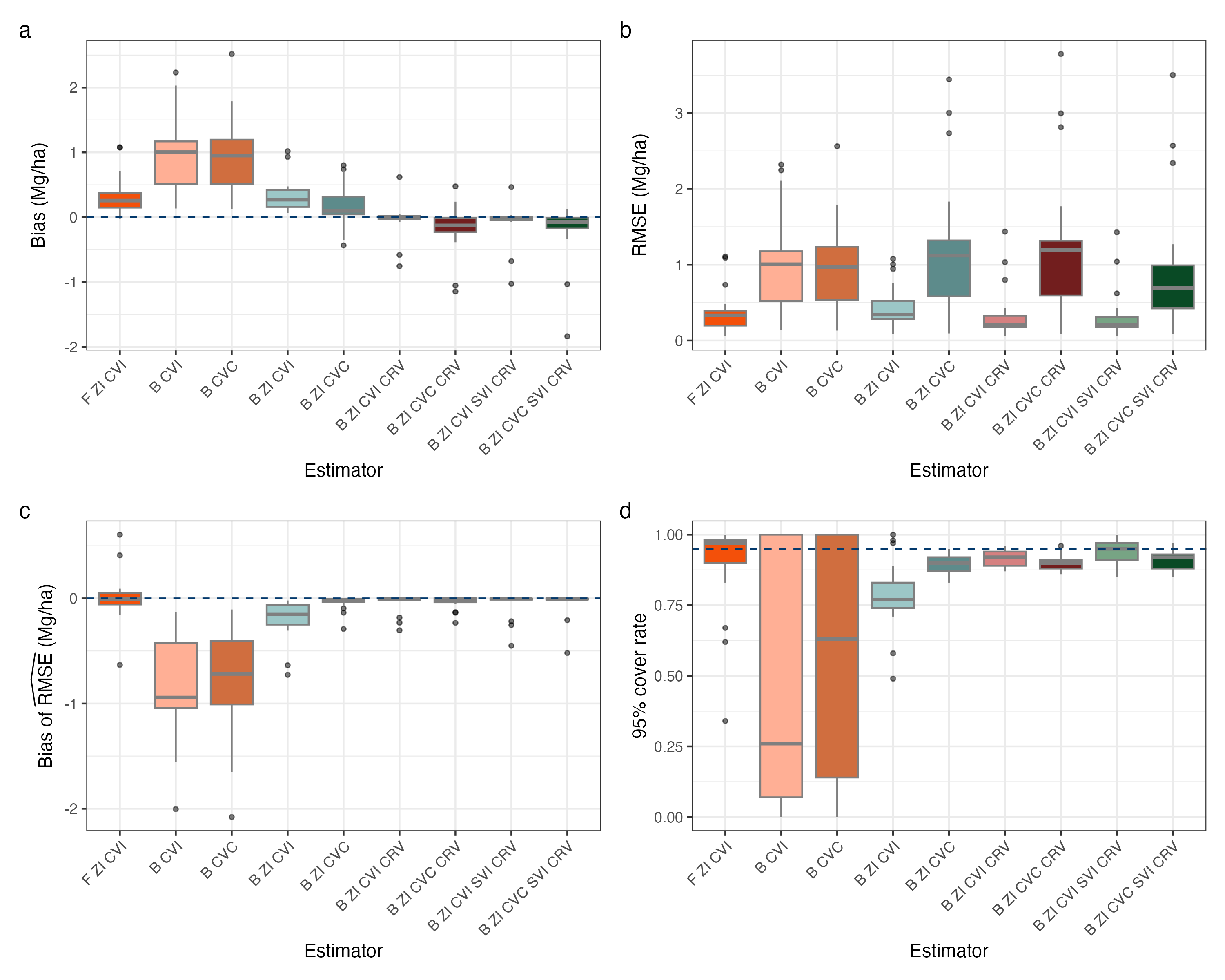
Figure 2 displays values for the four performance metrics evaluated in Washington, with each point on the plot represented a county-performance metric-estimator combination. Figure 2a displays the bias of each estimator, and we see in Washington that the F ZI CVI estimator exhibits the most bias, substantially more than its Bayesian counterpart. Initially this may come as a surprise due to the estimators similar structure, but one must consider the differences in the back-transformation of the response variable between these estimators. While the frequentist estimator back-transforms the predictions from each model, the Bayesian estimators back-transforms each sample from the posterior predictive distribution, potentially leading to more sensible estimates under certain conditions. The B CVI and B CVC estimators tend to exhibit greater magnitude bias than the two-stage Bayesian estimators, all of which exhibit similar amounts of bias to each other. One notable observation is the B ZI CVC CRV and B ZI CVC SVI CRV estimators exhibit a slight amount more bias than their CVI counterparts, and when we turn to Figure 2b we can see their RMSE is higher than their CVI counterparts. The B ZI CVI CRV and B ZI CVI SVI CRV estimators have the lowest RMSE, while the F ZI CVI estimator has the highest RMSE. Other two-stage Bayesian estimators exhibit very similar RMSE to each other, and the single-stage estimators exhibit a bit higher RMSE. Turning to Figure 2c, we see the bias of the RMSE estimator. Notably, the F ZI CVI and B CVI estimators exhibit the most bias here, while the other estimators exhibit very low bias. Once CRVs are accounted for, we see almost no bias. Finally, turning to Figure 2d, we examine the 95% uncertainty interval coverage rate. The B CVI and B CVC estimators have very poor coverage, while the other estimators, all of which are two-stage, have decent coverage among themselves. Notably, the estimators which account for CRVs and have CVC effects exhibit the best coverage rates.
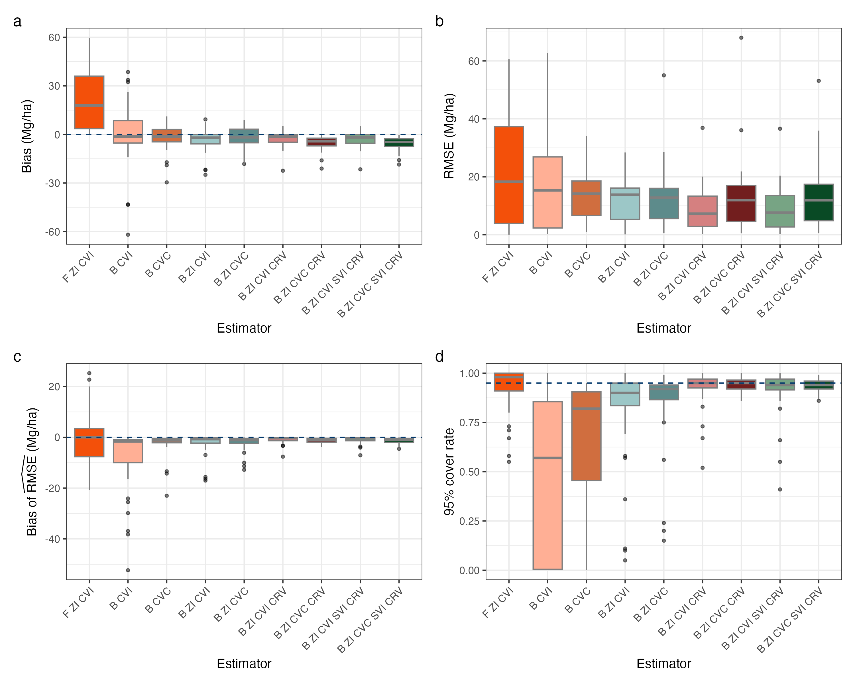
Stepping back from the details of Figures 1 and 2, we can gain some broader insights about the estimators and the simulation study. First of all, it is striking that the estimators that include a SVI perform almost identically to their non-spatial counterparts. This is not to say that spatial effects are unuseful for estimating biomass or other forest attributes, in fact we know from other studies these effects are quite useful (Finley et al.,, 2024). Further, from the cross-validation carried out in Section 3.2 we see more substantial improvements with the spatial models. It is the case though, that the simulated population we generated does not necessarily reflect the spatial structure of the true population, and in fact upon inspection it has very little spatial structure. Incorporating some spatial smoothing into the population generation methodology would help improve the simulated population’s utility for assessing these spatial models. Another broad observation we can make from the simulation study is that the CVCs generally did not improve estimation, and in some cases they worsened estimation. We see this particularly in Nevada, where county-level biomass is more homogeneous across the state. In Washington, the estimators with CVCs did have better 95% coverage rates than their CVI counterparts, but at the cost of higher bias and RMSE. The use of CVCs may be more useful for models fit across larger spatial domains (such as the entire United States), where we would expect the effect of predictors on the response to vary substantially. States with more diverse forest types may also benefit from the use of CVCs.
3.2 FIA data application
We applied the estimators discussed to actual plot data collected by FIA in both Nevada and Washington. We first compare the estimators using 10-fold cross-validation, and then turn to discussing estimates produced by the B ZI CVI SVI CRV estimator, an estimator that showed favorability in the simulation study and in cross-validation.
We performed 10-fold cross-validation at the unit-level to help assess the estimators performance, with the unit-level predictions as a proxy for estimation of county means. Results from the cross-validation are shown in Table 3. To compute 95% uncertainty interval coverage rates (“Coverage” in Table 3), we used the quantiles of the posterior predictive distribution of for the Bayesian estimators. We omit 95% confidence interval coverage for the frequentist estimators as the task of computing closed form or bootstrap prediction intervals at the unit-level for this two-stage model is beyond the scope of this article. Regarding the results, we can see similar patterns as we saw in Figures 1 and 2, but now we can better see the performance improvement associated with the spatial models when considering the root mean square prediction error (RMSPE) and bias. We see that across states bias and coverage rates were favorable for all estimators that included a county-specific variance term, and in Nevada for all estimators that account for zero-inflation. Examining the results of this cross-validation is helpful for model evaluation and in this case provides similar insights to the simulation study, and in Section 4 we discuss the tradeoffs of the two model evaluation methods.
| State | Metric | F ZI CVI | B CVI | B CVC | B ZI CVI | B ZI CVC | B ZI CVI CRV |
| WA | RMSPE | 107.05 | 113.90 | 111.48 | 106.87 | 104.78 | 104.03 |
| WA | Bias | 18.10 | 22.49 | 19.75 | 17.52 | 15.49 | -1.63 |
| WA | Coverage | NA | 42.95 | 49.10 | 65.00 | 69.41 | 96.77 |
| NV | RMSPE | 7.79 | 8.17 | 8.27 | 7.79 | 9.30 | 7.82 |
| NV | Bias | 0.35 | 0.85 | 0.88 | 0.33 | -0.24 | 0.00 |
| NV | Coverage | NA | 49.95 | 68.79 | 91.57 | 95.41 | 97.85 |
| State | Metric | B ZI CVC CRV | B ZI CVI SVI CRV | B ZI CVC SVI CRV |
| WA | RMSPE | 103.17 | 98.62 | 99.15 |
| WA | Bias | -3.21 | -2.15 | -3.71 |
| WA | Coverage | 96.59 | 96.71 | 96.68 |
| NV | RMSPE | 8.90 | 7.77 | 7.73 |
| NV | Bias | -0.35 | 0.00 | -0.02 |
| NV | Coverage | 97.99 | 98.04 | 97.92 |
In both Nevada and Washington, the B ZI CVI SVI CRV estimator performs quite well when considering all computed metrics in the simulation study and cross-validation, so we chose to use this estimator as an example for producing pixel-level predictions and county-level estimates in Washington and Nevada. Figure 3a, b show pixel-level estimates of biomass probability and Figure 3c, d show estimated biomass (Mg/ha) in both Washington and Nevada produced by the B ZI CVI SVI CRV estimator. While we are not particularly interested in the pixel-level predictions for the study at hand, these sorts of maps can be very useful for management at very small spatial scales, such as the stand level. In this Bayesian framework, not only do we have pixel-level predictions, but we also have pixel-level uncertainty predictions. Further, we can easily summarize these pixel level predictions to get estimates and uncertainty estimates for any area that may be of interest. For the study at hand, we only produce estimates for counties, but we could have just as easily produced estimates for any custom small area of interest (e.g., ecoregions, watersheds, fires, stands, etc.) with any of the Bayesian estimators.
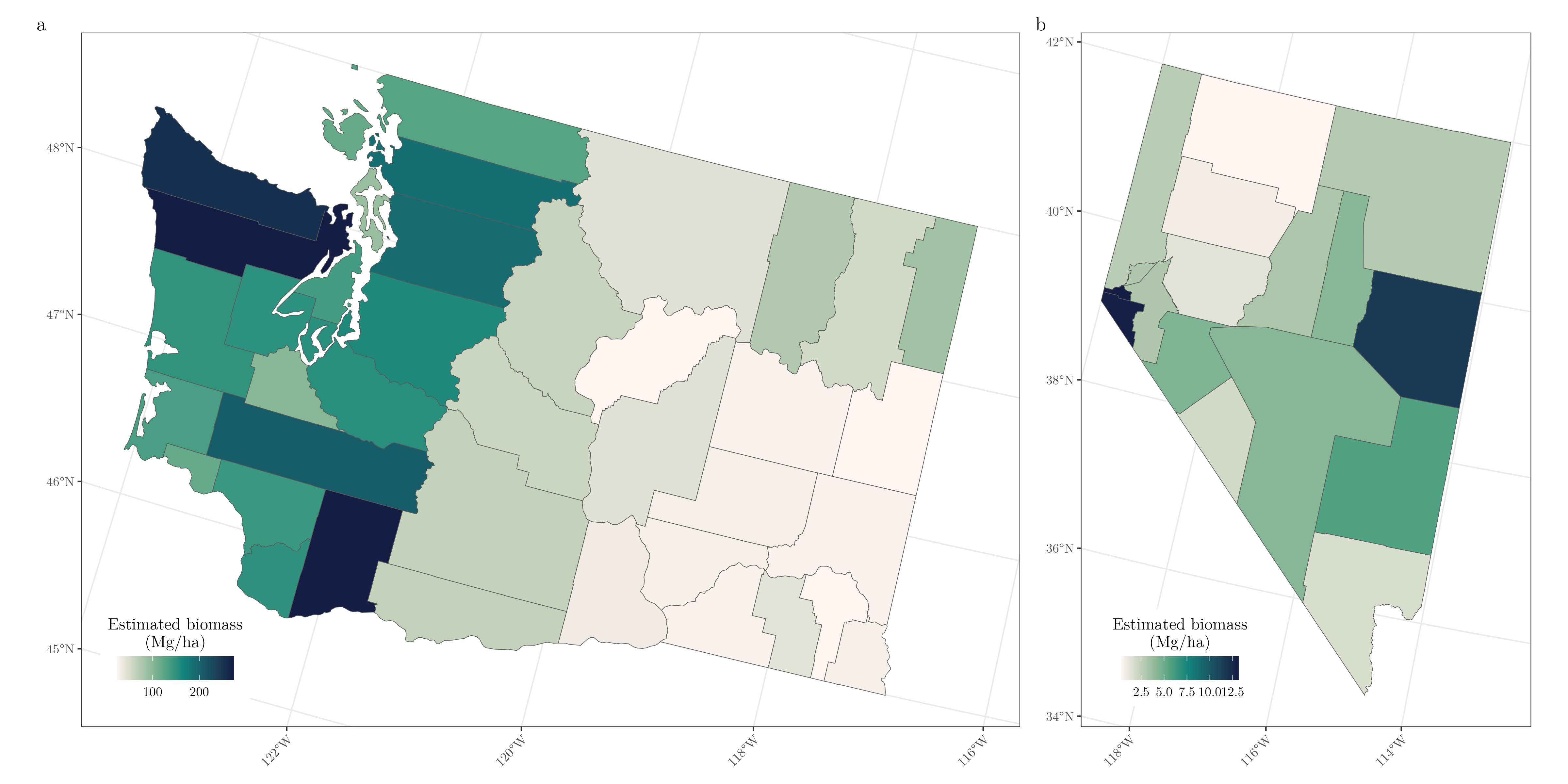
Figure 4 shows the estimated biomass (Mg/ha) in both Nevada and Washington produced by the B ZI CVI SVI CRV estimator. These sorts of estimates are what we are most interested for SAE, and for demonstration we only produce estimates at the county-level. County-level estimates of biomass show the stark change in biomass across the cascades in Washington state, and the relatively constant county-level biomass across the state of Nevada.
4 Discussion
Our work implemented and compared nine model-based approaches from both the frequentist and Bayesian statistical paradigms to estimating biomass in counties in the states of Nevada and Washington. The Bayesian estimators used allow for much flexibility in model specification, allowing for CVIs, CVCs, CRVs, and SVIs. We assessed the proposed estimators through a simulation study using design-based samples from a simulated population generated by a bootstrap-weighted NN technique, and through cross-validation at the unit-level on FIA data. Results suggest that accounting for zero inflation through a two-stage approach, the inclusion of CRVs, and the inclusion SVIs yield the best performing estimators.
It is an inherently difficult task to compare estimators for the purposes of SAE given to the small sample size in areas of interest and lack of true parameter values at the granularity of the area of interest. We implemented two methods for evaluating the proposed estimators, each of which have tradeoffs. First, we generated a simulated population for estimation evaluation. This approach allows for us to assess estimators empirically by sampling repeatedly from the simulated population and comparing estimates to the true value for the response in each county. These assessments are only insightful in the case that (1) the simulated population does not unfairly portray the estimators by being generated from some method too similar to the proposed estimators; and (2) the simulated population is similar enough to the true population that fitting these estimators to samples from the simulated population is representative of fitting the estimators to a sample of the true population. We achieve (1) here by using the bootstrap-weighted NN simulated population generation technique proposed by White et al., 2024a , but partially miss the mark regarding (2) as the simulated population does not have similar spatial structure to the true population, impeding our ability to accurately assess the models with a space varying intercept. Second, we used cross-validation to assess prediction made onto unit-level observations. This approach does not require assumptions about how the population is generated or otherwise, but only allows for assessment of unit-level predictions. In our case, the cross-validation analysis yielded very similar results to the simulation study, and we were able to more clearly see the benefit of the spatial models. However, cross-validation is only possible for unit-level small area estimators and we must tolerate unit-level predictions as a proxy for small area estimates.
Our analyses provide insight as to how we may want to go about estimating biomass, or other continuous zero-inflated forest attributes, in areas of mixed landscape types and how a practitioner may want to assess their modeling choices. Given our changing climate and increasingly prolific disturbances, such as fires, producing accurate estimates of forest attributes in small areas that are zero-inflated is of the upmost importance understanding our ever-changing landscape. In future work, we hope to test the proposed estimators across a variety of regions such as recently burned areas, forest stands, and other areas with great ecological importance. Further, we hope to improve our methodology for creating simulated populations in order to better assess the quality of spatial area- and unit-level small area estimators. We also hope to consider temporal effects in these zero-inflated estimators, to be able to estimate change in biomass across time scales.
Author statements
Acknowledgments
The authors thank the Forest Inventory & Analysis Program for the data.
Funding statement
This work was supported by the USDA Forest Service Forest Inventory and Analysis Program, Region 9, Forest Health Protection, Michigan State University AgBioResearch, National Science Foundation DEB-2213565 and DEB-1946007, and National Aeronautics and Space Administration CMS Hayes-2023. The findings and conclusions in this publication are those of the authors and should not be construed to represent any official US Department of Agriculture or US Government determination or policy.
Data availability statement
The data include confidential plot data, which can not be shared publicly. FIA data can be accessed through the FIA DataMart (https://apps.fs.usda.gov/fia/datamart/datamart.html). Requests for data used here or other requests including confidential data should be directed to FIA’s Spatial Data Services (https://www.fs.usda.gov/research/programs/fia/sds).
References
- Battese et al., (1988) Battese, G. E., Harter, R. M., and Fuller, W. A. (1988). An error-components model for prediction of county crop areas using survey and satellite data. Journal of the American Statistical Association, 83(401):28–36.
- Burrill et al., (2023) Burrill, E., Christensen, G., Conkling, B., DiTommaso, A., Lepine, L., Perry, C., Pugh, S., Turner, J., Walker, D., and Williams, M. (2023). Forest inventory and analysis database: Database description and user guide for phase 2 (version: 9.1).
- Cao et al., (2022) Cao, Q., Dettmann, G. T., Radtke, P. J., Coulston, J. W., Derwin, J., Thomas, V. A., Burkhart, H. E., and Wynne, R. H. (2022). Increased precision in county-level volume estimates in the united states national forest inventory with area-level small area estimation. Frontiers in Forests and Global Change, 5:769917.
- Chandra and Sud, (2012) Chandra, H. and Sud, U. C. (2012). Small area estimation for zero-inflated data. Communications in Statistics - Simulation and Computation, 41:632 – 643.
- Daly et al., (2002) Daly, C., Gibson, W. P., Taylor, G. H., Johnson, G. L., and Pasteris, P. (2002). A knowledge-based approach to the statistical mapping of climate. Climate Research, 22(2):99–113.
- Datta et al., (2016) Datta, A., Banerjee, S., Finley, A. O., and Gelfand, A. E. (2016). Hierarchical nearest-neighbor Gaussian process models for large geostatistical datasets. Journal of the American Statistical Association, 111(514):800–812.
- Fay and Herriot, (1979) Fay, R. E. I. and Herriot, R. A. (1979). Estimates of income for small places: an application of james-stein procedures to census data. Journal of the American Statistical Association, 74(366a):269–277.
- Finley, (2025) Finley, A. O. (2025). Models for zero-inflated data.
- Finley et al., (2024) Finley, A. O., Andersen, H.-E., Babcock, C., Cook, B. D., Morton, D. C., and Banerjee, S. (2024). Models to support forest inventory and small area estimation using sparsely sampled lidar: A case study involving g-liht lidar in tanana, alaska. Journal of Agricultural, Biological and Environmental Statistics, 29(4):695–722.
- Finley et al., (2011) Finley, A. O., Banerjee, S., and MacFarlane, D. W. (2011). A hierarchical model for quantifying forest variables over large heterogeneous landscapes with uncertain forest areas. Journal of the American Statistical Association, 106(493):31–48.
- Finley et al., (2019) Finley, A. O., Datta, A., Cook, B. D., Morton, D. C., Andersen, H. E., and Banerjee, S. (2019). Efficient algorithms for Bayesian nearest neighbor Gaussian processes. Journal of Computational and Graphical Statistics, 28(2):401–414.
- Gelman et al., (2013) Gelman, A., Carlin, J., Stern, H., Dunson, D., Vehtari, A., and Rubin, D. (2013). Bayesian Data Analysis, Third Edition. Chapman & Hall/CRC Texts in Statistical Science. Taylor & Francis.
- May et al., (2023) May, P., McConville, K. S., Moisen, G. G., Bruening, J., and Dubayah, R. (2023). A spatially varying model for small area estimates of biomass density across the contiguous united states. Remote Sensing of Environment, 286:113420.
- Pfeffermann et al., (2008) Pfeffermann, D., Terryn, B., and Moura, F. (2008). Small area estimation under a two-part random effects model with application to estimation of literacy in developing countries. Survey Methodology, 34.
- Picotte et al., (2019) Picotte, J. J., Dockter, D., Long, J., Tolk, B., Davidson, A., and Peterson, B. (2019). LANDFIRE remap prototype mapping effort: Developing a new framework for mapping vegetation classification, change, and structure. Fire, 2(2):35.
- Prisley et al., (2021) Prisley, S., Bradley, J., Clutter, M., Friedman, S., Kempka, D., Rakestraw, J., and Sonne Hall, E. (2021). Needs for small area estimation: Perspectives from the us private forest sector. Frontiers in Forests and Global Change, 4:746439.
- R Core Team, (2024) R Core Team (2024). R: A Language and Environment for Statistical Computing. R Foundation for Statistical Computing, Vienna, Austria.
- Rao and Molina, (2015) Rao, J. and Molina, I. (2015). Small Area Estimation. Wiley, 2nd edition. ISBN: 978-1-118-73578-7.
- Rollins, (2009) Rollins, M. G. (2009). LANDFIRE: a nationally consistent vegetation, wildland fire, and fuel assessment. International Journal of Wildland Fire, 18(3):235–249.
- U.S. Geological Survey, (2019) U.S. Geological Survey (2019). LANDFIRE Elevation.
- U.S. Senate, (2023) U.S. Senate (2023). S. Rep. 118-83 - Department of the Interior, Environment, and Related Agencies Appropriations Bill.
- (22) White, G. W., Wieczorek, J. A., Cody, Z. W., Tan, E. X., Chistolini, J. O., McConville, K. S., Frescino, T. S., and Moisen, G. G. (2024a). Assessing small area estimates via bootstrap-weighted k-nearest-neighbor artificial populations.
- (23) White, G. W., Wieczorek, J. A., Frescino, T. S., and McConville, K. S. (2024b). kbaabb: Generates an Artificial Population Based on the KBAABB Methodology. R package version 0.0.0.9000.
- White et al., (2025) White, G. W., Yamamoto, J. K., Elsyad, D. H., Schmitt, J. F., Korsgaard, N. H., Hu, J. K., Gaines, G. C., Frescino, T. S., and McConville, K. S. (2025). Small area estimation of forest biomass via a two-stage model for continuous zero-inflated data. Canadian Journal of Forest Research, 0(ja):null.
- Wiener et al., (2021) Wiener, S. S., Bush, R., Nathanson, A., Pelz, K., Palmer, M., Alexander, M. L., Anderson, D., Treasure, E., Baggs, J., and Sheffield, R. (2021). United states forest service use of forest inventory data: Examples and needs for small area estimation. Frontiers in Forests and Global Change, 4:763487.
- Yamamoto et al., (2025) Yamamoto, J., Elsyad, D., White, G., Schmitt, J., Korsgaard, N., McConville, K., and Hu, K. (2025). saeczi: Small Area Estimation for Continuous Zero Inflated Data. R package version 0.2.0.9000, commit f580319049b152c890033c770913b7a296ce63cb.
- Yang et al., (2018) Yang, L., Jin, S., Danielson, P., Homer, C., Gass, L., Bender, S. M., Case, A., Costello, C., Dewitz, J., Fry, J., Funk, M., Granneman, B., Liknes, G. C., Rigge, M., and Xian, G. (2018). A new generation of the United States National Land Cover Database: Requirements, research priorities, design, and implementation strategies. ISPRS Journal of Photogrammetry and Remote Sensing, 146:108–123.
Appendix
Appendix A Prior distributions and hyperparameters
Table 4 includes the prior distribution and hyperparameter values for all parameters use for the Bayesian models.
| Parameter | Prior distribution | hyperparameter values |
| None | Set to 0.00001 |