HIF: Height Interval Filtering for Efficient Dynamic Points Removal
Abstract
3D point cloud mapping plays a essential role in localization and autonomous navigation. However, dynamic objects often leave residual traces during the map construction process, which undermine the performance of subsequent tasks. Therefore, dynamic object removal has become a critical challenge in point cloud based map construction within dynamic scenarios. Existing approaches, however, often incur significant computational overhead, making it difficult to meet the real-time processing requirements. To address this issue, we introduce the Height Interval Filtering (HIF) method. This approach constructs pillar-based height interval representations to probabilistically model the vertical dimension, with interval probabilities updated through Bayesian inference. It ensures real-time performance while achieving high accuracy and improving robustness in complex environments. Additionally, we propose a low-height preservation strategy that enhances the detection of unknown spaces, reducing misclassification in areas blocked by obstacles (occluded regions). Experiments on public datasets demonstrate that HIF delivers a improvement in time efficiency with comparable accuracy to existing SOTA methods. The code will be publicly available.
I Introduction
As a fundamental type of observations utilized in Simultaneous Localization and Mapping (SLAM) systems, 3D point cloud has demonstrate significant potential to impact a diverse range of applications [1, 2]. In most cases, point cloud maps are constructed through a mapping process in LiDAR-equipped SLAM systems. However, complex urban environments often feature a multitude of dynamic objects, including moving vehicles, cyclists, and pedestrians, which leave residual artifacts (or ghost traces), during the mapping process, thereby significantly affecting the construction quality [3, 4]. With the rapid development of point cloud mapping, a common technique is to remove dynamic objects during the mapping process.
Traditionally, dynamic point removal is often implemented using ray casting. However, this approach relies heavily on computationally intensive retrieval processes, involving point-by-point operations that require traversing each voxel, making it challenging to meet real-time requirements. Moreover, due to the small pitch angle between the rays and the distant ground surface, this method is prone to misclassifying ground points, leading to incorrect removals [5, 6].
Recent studies [7, 6, 8, 9, 10, 5] have formulated dynamic object removal as detecting occupancy differences between consecutive frames. However, most of these approaches operate as post-processing methods, requiring all scans to be treated as global priors to ensure accuracy, which prevents real-time execution. Additionally, some methods employ egocentric map representations that lack global consistency, necessitating extra transformations from global map points to the local frame [10], thereby introducing significant computational overhead. Moreover, many of these approaches rely on ground segmentation modules, further increasing both computational complexity and system intricacy.
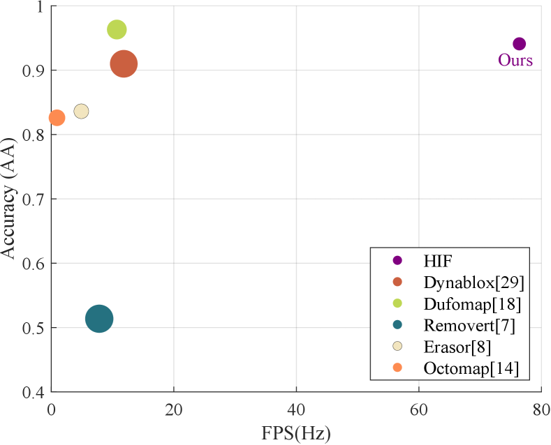
In this paper, we propose a dynamic point cloud removal method, termed Height Interval Filtering (HIF). This method partitions the space into globally consistent pillars and employs a hash-mixed indexing operation to reduce retrieval dimensions and collision rates, thereby significantly enhancing retrieval efficiency. Simultaneously, we establish height intervals to discretize the vertical space and assign probability values to them, which are then refined through Bayesian filtering. Our method eliminates the reliance on ray-tracing and ground point segmentation modules, significantly accelerating computation and enabling efficient real-time operation. In real-world scenarios, complex occlusions in the environment often hinder the performance of ray-casting-based dynamic object removal algorithms, leading to decreased accuracy and efficiency. To address this, we introduce a low-height preservation strategy, which exploits the spatial structure of pillars to identify unknown spaces in the scan, thereby improving robustness in complex environments. To validate the effectiveness of our method, we conducted experiments on the KITTI [11] datasets with annotation labels and poses from SemanticKITTI [12] and Argoverse 2 [13] datasets. As shown in Fig. 1, our method achieves a 6-7× increase in FPS compared to recent methods, while maintaining high accuracy in dynamic object removal.
Briefly, we identify our contributions as follows
-
•
An efficient Height Interval Filtering (HIF) approach that assigns probabilities to height intervals to model vertical structures, ensuring both efficiency and accuracy in dynamic point cloud removal.
-
•
A low-height preservation strategy to reduce misclassification in occluded regions by identifying unknown spaces in each scan.
-
•
Evaluated on the KITTI and AV2 datasets, the proposed HIF algorithm achieves exceptional computational efficiency while preserving high accuracy.
II Related Works
II-A FreeSpace-based Removal methods
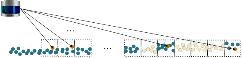
FreeSpace-based removal methods represent point clouds as voxels and update occupancy states using per-frame scan results based on ray-tracing principles [14, 15]. However, sole reliance on ray-tracing leads to significant misclassification issues, particularly affecting ground points, as shown in Fig. 2. To address this, some methods incorporate post-processing techniques to recover ground points after ray-tracing, effectively reducing misclassification errors [16, 17]. Additionally, improvements in trace efficiency and the introduction of more robust discriminative mechanisms have further enhanced both computational efficiency and accuracy [18, 19]. Despite these advancements, computationally expensive 3D retrieval remains a major bottleneck for real-time performance. Our approach mitigates this by partitioning the space into pillars and transforming 3D retrieval into a more efficient 1D lookup using a hash-mixed operation, significantly reducing computational complexity.
II-B Difference-based methods
Difference-based methods detect dynamic objects by analyzing visibility or disparity changes. One approach involves converting maps into depth images and comparing depth differences between frames and a global map, as demonstrated in [7, 5]. Other methods prioritize vertical information, detecting changes along the vertical axis to identify dynamic objects [8, 9, 10, 6]. Some techniques employ vertical layering, which can lead to rigid height stratification issues. Most difference-based approaches operate as post-processing techniques, requiring all scans as global priors to ensure accuracy, thereby limiting real-time applicability. Additionally, these methods heavily depend on ground segmentation, increasing computational overhead and system complexity. In contrast, our approach models vertical distributions by constructing flexible height intervals, eliminating reliance on ground segmentation and mitigating rigid height stratification issues.
II-C learning-based methods
Learning-based methods have shown strong capabilities across various domains. In dynamic object removal, the task is often reformulated as a point cloud segmentation problem [20, 21, 22]. These approaches transform point clouds into range images to achieve a dense and compact representation [20, 21]. More recent methods introduce residual images to incorporate dynamic information, improving segmentation performance [23, 24, 25, 26, 27]. However, learning-based approaches require extensive training data and suffer from data imbalance issues [28], while generalization and robustness remain significant challenges [18]. Furthermore, their high computational cost limits practical deployment.
III Methodology
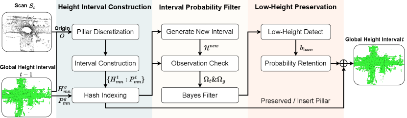
We propose Height Interval Filtering (HIF) for dynamic point removal, as illustrated in Fig. 3. HIF consists of three key steps: height interval construction (Section III-A), interval probability filtering (Section III-B), and low-height preservation (Section III-C). Upon acquiring a new point cloud scan, it is transformed into a height interval representation using a globally consistent partitioning scheme, with global height intervals updated via Bayesian filtering. The proposed low-height preservation strategy identifies unknown space in the scan, improving retention of static structures in highly occluded environments. Finally, dynamic points are removed by preserving those within height intervals with high static probabilities.
III-A Height Interval Construction
Recent studies [8, 9, 10, 6] have demonstrated that analyzing vertical information effectively aids in dynamic object identification. Inspired by these works, we adopt a pillar-based representation to capture vertical structures. Within each pillar, we construct height intervals to model spatial occupancy probabilities. To ensure a globally consistent pillar partitioning, we define a fixed origin point on the XY plane, preventing misalignment between new scans and the global height intervals.
In our approach, we represent the environment using a 2D pillar-based grid where each pillar has a fixed size of in the XY plane. These pillars are used to discretize the space horizontally, while vertical information is modeled by constructing height intervals within each pillar to maintain spatial occupancy probabilities.
At time , the point cloud scan is denoted as , where represents the total number of points in the scan. Each point is assigned to a corresponding pillar by computing its offset relative to the global origin . The offset is determined as follows:
| (1) |
This scheme ensures the pillar boundaries align with:
| (2) |
To enable efficient pillar retrieval, we employ a hash-mixed operation to generate unique pillar indices:
| (3) |
where represents a standard integer hash function, is a constant derived from the golden ratio, commonly used in hash functions to improve distribution uniformity. The operators and denote bitwise left and right shifts, respectively.
This hashing strategy ensures an injective mapping, minimizing the risk of collisions. Furthermore, to optimize storage efficiency, we store only non-empty pillars and construct an index for fast access.
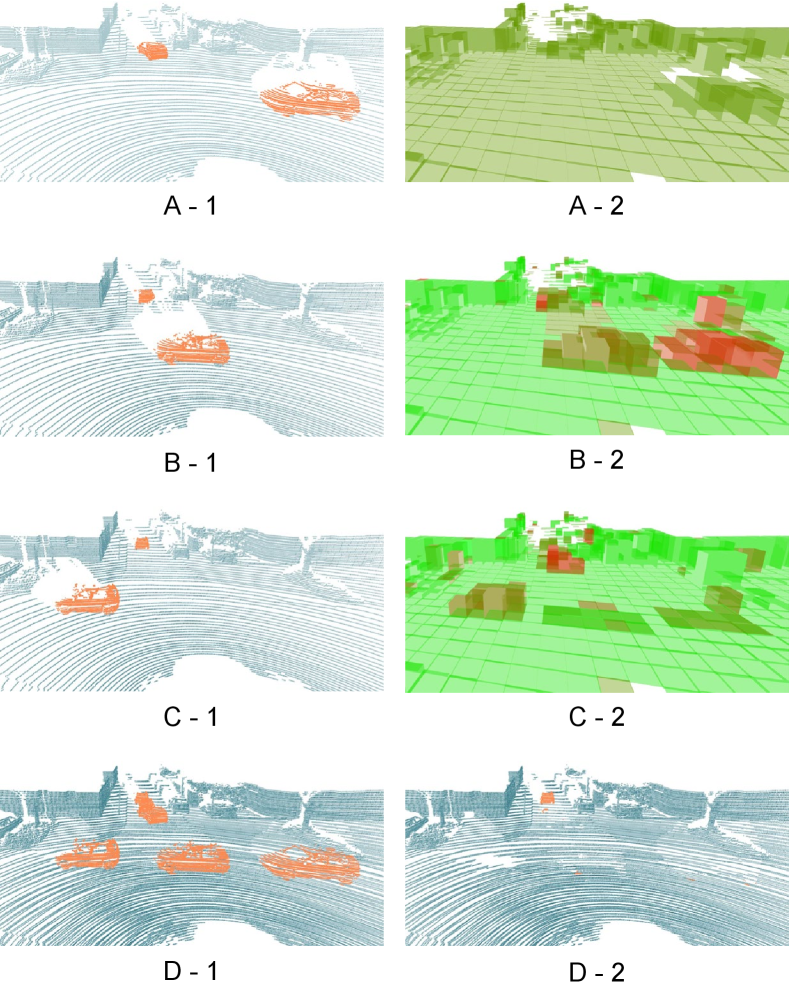
Next, our approach dynamically merges height values within each pillar into adaptive height intervals, enabling finer vertical representation without requiring ground segmentation, as illustrated in Fig. 4 A-1 and Fig. 4 A-2. This design addresses the limitations of existing methods, which suffer from rigid vertical partitioning. The R-POD method in [8] and the approaches in [9, 10] rely on predefined height divisions with binary or symbolic encoding, making them less adaptable to elevation changes and occlusions. Additionally, these methods require auxiliary ground segmentation and lack probabilistic modeling, leading to potential misclassifications in complex scenes.
We define to maintain the occupancy probability of the empty space in each pillar, which provides reasonable initialization for the observed height interval in new scans. Each pillar is structured as follows:
| (4) |
where the set represents the collection of height intervals within a pillar, containing discrete height intervals . Each interval is defined by three parameters: and , which denote the minimum and maximum height values within the interval, respectively, and , which represents the occupancy probability of the interval.
We represent each pillar using an index and an associated storage variable , forming a key-value pair . To maintain a global mapping of pillars, we define a dictionary , where denotes the spatial index of a pillar in the global map, and stores its corresponding height intervals and occupancy probabilities. Upon receiving a new scan at time , we perform the Height Interval Construction operation to generate a local pillar set , where represents the spatial index of a pillar in the current scan, and contains its associated height intervals and occupancy probabilities.
For each newly generated local pillar pair in , we first check whether a corresponding global pillar exists in . If a match is found, we update using following the probability filtering operations described in Sections III-B and III-C. If no match is found, the new key-value pair is directly inserted into .
III-B Interval Probability Filtering
We employ a binary Bayes filter to update the occupancy probability of height interval. The observation model parameters are determined by the height interval’s observation status in the new scan and global mapping of pillars:
| (5) |
| (6) | |||
where and are empirically determined confidence parameters (, ).
When is successfully matched with in the new scan, it confirms that has been observed. Consequently, we update the occupancy probability of empty space within using Eq. 7, thereby reducing the likelihood of it being occupied:
| (7) |
We extract all height interval endpoints from and to construct the set of interval endpoints. Specifically, we extract and from the height intervals in , where and denote the minimum and maximum height values of the -th interval in , respectively. Similarly, we take and from all height intervals in , where and represent the minimum and maximum height values of the -th interval in , respectively. The resulting interval endpoint set is defined as:
| (8) |
After sorting these endpoints into an ordered sequence where , we generate new height intervals through pairwise combination:
| (9) |
For each new interval , we determine its temporal correspondence by analyzing overlaps with existing height intervals. Specifically, we define and to represent the observation states of the new height interval within and , respectively:
| (10) | ||||
When , this means that the interval is not covered by any historical or current observations, thus we discard this interval. When , it indicates that we have consistent observations, so we apply the Bayesian filter to increase the occupancy probability based on :
| (11) |
When , the height interval exists in the global pillar but remains unobserved in the current scan . Consequently, its occupancy probability is reduced based on :
| (12) |
When , we update the probability based on as the static probability for the new height interval:
| (13) |
| KITTI 00 | KITTI 02 | KITTI 05 | AV2 | |||||||||
|---|---|---|---|---|---|---|---|---|---|---|---|---|
| Methods | SA(%) | DA(%) | AA(%) | SA(%) | DA(%) | AA(%) | SA(%) | DA(%) | AA(%) | SA(%) | DA(%) | AA(%) |
| Removert[7] | 99.56 | 37.33 | 60.97 | 96.67 | 39.08 | 61.47 | 99.48 | 26.52 | 51.37 | 98.97 | 31.16 | 55.53 |
| Erasor[8] | 70.41 | 98.26 | 83.18 | 50.76 | 98.60 | 70.74 | 70.79 | 98.75 | 83.61 | 77.51 | 99.18 | 87.68 |
| Octomap[14] | 69.57 | 99.71 | 83.29 | 62.61 | 98.55 | 78.55 | 69.37 | 98.34 | 82.60 | 69.04 | 97.50 | 82.04 |
| Dynablox[29] | 99.72 | 89.47 | 94.46 | 83.07 | 94.86 | 88.77 | 99.34 | 83.34 | 90.99 | 99.35 | 86.08 | 92.48 |
| Dufomap[18] | 98.64 | 98.53 | 98.58 | 68.56 | 98.47 | 82.16 | 97.18 | 95.44 | 96.31 | 96.67 | 88.90 | 92.70 |
| HIF(Ours) | 98.40 | 95.46 | 96.92 | 97.66 | 85.62 | 91.44 | 98.11 | 90.23 | 94.09 | 83.47 | 84.17 | 83.82 |
III-C Low-Height Preservation Strategy
In our approach, we propose the Low-Height Preservation (LHP) strategy, which leverages the spatial characteristics of the pillar-based structure to prevent incorrect updates of unknown space in a new scan. Specifically, when matching indices between and , we traverse each height interval in , denoted as for . We then extract the minimum and define it as the base height of the current pillar.
This has two possible physical interpretations:
-
1.
It may correspond to the ground level observed within the pillar.
-
2.
Alternatively, it could be the lowest detected point, constrained by occlusion from objects in the foreground.
The region below is treated as unknown space in the current scan.
To define the lowest base point, we extract the minimum value from all height intervals in , using the following formula:
| (14) |
When updating the global height intervals, we apply the Low-Height Preservation (LHP) strategy, maintaining the occupancy probability for the interval as:
| (15) |
To prevent excessive probability convergence, we apply a bounded update:
| (16) |
Finally, we replace the height intervals in the global pillar with the updated set :
| (17) |
where denotes the element-wise probability clipping operation.
IV Experiment
Our experiments include Experimental Setup for method selection and parameters, Evaluation Datasets for dataset configurations, Evaluation Metrics for assessment criteria, Accuracy and Runtime Evaluation for performance analysis, and Ablation Study for key parameter impact.
IV-A Experimental Setup
We classify the compared methods into online and offline approaches, selecting representative works from each category. For offline methods, we include Removert, ERASOR, and the latest SOTA method, DUFOMap. For online methods, we evaluate the classic OctoMap and Dynablox.
For parameter settings, we use the benchmark configurations from [16] for Removert, ERASOR, and Dynablox. OctoMap is set with a voxel size of 0.1 meters. For DUFOMap, we follow the original paper’s parameters, using a voxel size of 0.1 meters, meters, and a sub-voxel localization error of .
For our method, we set the pillar size to 1 meter along both the X and Y axes. For different datasets, we only fine-tuned the observation model parameters and .
All experiments were conducted on a desktop computer equipped with an Intel Core i9-13900KF processor and 64GB of RAM.
IV-B Evaluation Datasets
To validate the effectiveness of our algorithm, we conducted a precision evaluation and runtime evaluation using the KITTI dataset, with ground truth labels provided by Semantic KITTI. The dataset is captured using the HDL-64E LiDAR and includes pose and point cloud labels. Following the setup in [8] and [16], we selected sequences 00 (frames 4,390 - 4,530), 01 (frames 150 - 250), 02 (frames 860 - 950), and 05 (frames 2,350 - 2,670). During preprocessing, we discarded points labeled as 0 (unknown) and 1 (unlabeled).
To evaluate the adaptability of our algorithm to different sensors, we conducted supplementary experiments on the Argoverse 2 dataset, which utilizes the VLP-32C LiDAR. The dataset setup follows the configuration in [16].
| KITTI 00 | KITTI 01 | KITTI 02 | KITTI 05 | KITTI 07 | |||||||||||
|---|---|---|---|---|---|---|---|---|---|---|---|---|---|---|---|
| Methods | Mean | Std | FPS | Mean | Std | FPS | Mean | Std | FPS | Mean | Std | FPS | Mean | Std | FPS |
| Removert[7] | 56.74 | 1.149 | 17.62 | 39.07 | 0.925 | 25.60 | 38.07 | 0.49 | 26.27 | 127.7 | 2.615 | 7.831 | 76.87 | 1.517 | 13.01 |
| Erasor[8] | 105.3 | 13.31 | 9.497 | 708.2 | 40.35 | 1.412 | 98.20 | 24.32 | 10.18 | 203.9 | 19.69 | 4.904 | 57.52 | 12.33 | 17.39 |
| Octomap[14] | 887.5 | 92.95 | 1.126 | 2225 | 665.4 | 0.494 | 733.5 | 73.71 | 1.363 | 1077 | 121.7 | 0.929 | 792.4 | 71.85 | 1.262 |
| Dynablox[29] | 79.13 | 13.41 | 12.64 | 180.7 | 49.52 | 5.534 | 81.85 | 17.88 | 12.22 | 84.49 | 14.81 | 11.84 | 74.10 | 10.85 | 13.50 |
| Dufomap[18] | 98.01 | 16.85 | 10.20 | 127.7 | 21.10 | 7.831 | 83.80 | 17.68 | 11.93 | 93.46 | 19.61 | 10.70 | 81.20 | 20.03 | 12.32 |
| HIF(Ours) | 11.62 | 0.878 | 86.06 | 12.05 | 1.784 | 82.99 | 11.70 | 1.310 | 90.33 | 13.09 | 1.809 | 76.39 | 13.32 | 1.957 | 75.08 |
IV-C Evaluation Metrics
We follow the evaluation approach of [16], using point-level static accuracy (SA) and dynamic accuracy (DA) to directly measure the algorithm’s performance, avoiding the need for ground truth downsampling. Additionally, we employ Associated Accuracy (AA) as a comprehensive metric, defined in Eq. 18, to ensure sensitivity to both static and dynamic points:
| (18) |
For runtime evaluation, we measure the average runtime per frame and FPS to assess computational efficiency, while the standard deviation of runtime is used to evaluate the algorithm’s stability.
IV-D Accuracy Evaluation
We evaluated our method on the KITTI and AV2 datasets, with results presented in Table I. Removert achieves high static accuracy (SA) but struggles with dynamic accuracy (DA), indicating difficulty in detecting dynamic objects, whereas ERASOR and OctoMap perform well in dynamic object detection but suffer from significant misclassification, leading to lower static accuracy. Dynablox, DUFOMap, and our method HIF maintain a good balance between static and dynamic accuracy, with HIF ranking just below the SOTA method DUFOMap on KITTI while achieving the best performance on KITTI 02, and on AV2, the primary gap between HIF and DUFOMap lies in static accuracy, which we further analyze in the following visualization.
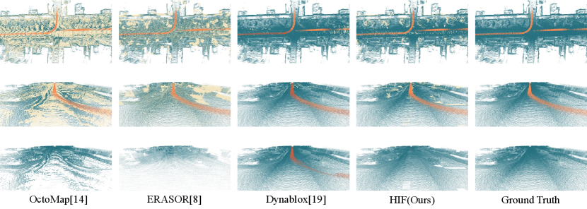
First, we selected the representative KITTI 05 sequence from the KITTI dataset for visualization, as shown in Fig. 5. OctoMap and ERASOR exhibit significant misclassification issues: the former frequently misclassifies ground points, while the latter suffers from sparse ground point retention due to insufficient preservation in the segmentation module, leading to entire pillars being misclassified. Dynablox excels in retaining static points but struggles with detecting dynamic objects. In contrast, our method, HIF, achieves strong performance for both static and dynamic points, with only minor misclassification observed at the top of the canopy.
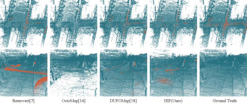
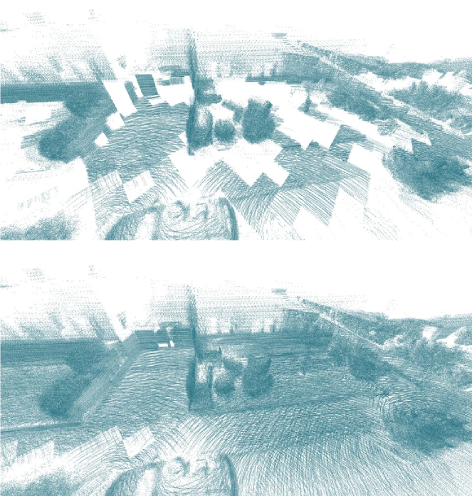
Then, as shown in Fig. 6, Removert effectively retains static points but struggles with dynamic object removal. Compared to the SOTA method DUFOMap, our approach shows weaker performance in high-rise buildings and canopy areas, with more frequent misclassifications. This is primarily due to the fact that in actual scan data, higher regions appear less frequently within their respective pillars due to occlusions or radar scanning angle limitations, leading to an incorrect reduction in static probabilities.
IV-E Runtime Evaluation
We evaluated the runtime of all methods on the KITTI sequences, with the results presented in Table II. Our method demonstrated a significant advantage across all sequences, achieving a speedup of several times compared to other approaches. Notably, its runtime remains consistent across different sequences, indicating stable performance across varying environments, whether open or narrow. Furthermore, the per-frame runtime variation is minimal, with low variance, highlighting the method’s robustness. The combination of fast execution and high stability makes our algorithm well-suited for integration into existing SLAM systems, enhancing performance without introducing instability.
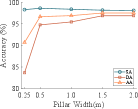
To analyze the influence of pillar width on both accuracy and computational efficiency, we conducted a series of experiments (Fig. 7). When the pillar width is small, a high miss rate is observed in dynamic object detection. As the width increases, dynamic accuracy (DA) improves and converges to 95.5%, while static accuracy (SA) remains nearly unchanged.
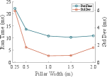
Furthermore, when the pillar width is small, the algorithm exhibits higher runtime and greater variance. In contrast, at 1 meter and 1.5 meters, the algorithm achieves the best runtime performance.
Additionally, we found that regardless of the pillar width, the algorithm’s peak memory usage remained stable at 801 ± 1MB, indicating high memory efficiency. The maximum memory consumption is primarily determined by the scale of the point cloud in the scene rather than the pillar width.
IV-F Ablation Study
Since Height Interval Construction and Interval Probability Filtering form the core components of our approach, we conduct ablation experiments exclusively on the Low-Height Preservation (LHP) module. To evaluate its effectiveness, we test this module across all data sequences.
| Seq | LHP | SA(%) | DA(%) | AA(%) |
|---|---|---|---|---|
| 00 | w/o | 91.00 | 95.48 | 93.22 |
| w/ | 98.40 | 95.46 | 96.92 | |
| 01 | w/o | 97.78 | 65.23 | 79.86 |
| w/ | 99.20 | 63.82 | 79.57 | |
| 02 | w/o | 64.25 | 90.68 | 76.33 |
| w/ | 97.66 | 85.62 | 91.44 | |
| 05 | w/o | 94.00 | 90.52 | 92.24 |
| w/ | 98.11 | 90.23 | 94.09 | |
| 07 | w/o | 92.84 | 68.92 | 79.99 |
| w/ | 99.00 | 65.38 | 80.46 | |
| AV2 | w/o | 74.08 | 85.23 | 79.46 |
| w/ | 83.47 | 84.17 | 83.82 |
Results presented in Table III, showing that while LHP has a negligible impact on dynamic accuracy (DA), it significantly improves static accuracy (SA); to further investigate this effect, we visualized the results for the KITTI 02 sequence in Fig. 8, where the complex scene—featuring parked vehicles, bushes, and occluded objects—leads to relatively low static accuracy for most algorithms, as shown in Table I, whereas our LHP strategy effectively identifies these occlusions and preserves static points in occluded areas.
V Conclusions
In this paper, we introduced HIF, a novel dynamic object removal framework that models occupancy probabilities along the vertical direction. Our method constructs pillar-based height interval representations, enabling efficient spatial partitioning, and employs Bayesian filtering to iteratively update interval probabilities. Additionally, the proposed low-height preservation (LHP) strategy effectively detects unknown spaces, improving robustness in highly occluded environments.
Experimental results demonstrate that HIF achieves state-of-the-art runtime efficiency while maintaining high accuracy, outperforming conventional methods in both computational speed and stability. However, certain limitations remain: misclassification can occur when high-altitude regions are observed less frequently than their corresponding pillars, and dynamic objects may be missed in areas with low observation frequency. Future work will focus on refining the pillar representation and exploring adaptive filtering techniques to further improve accuracy and robustness in diverse real-world scenarios.
References
- [1] T. Shan, B. Englot, D. Meyers, W. Wang, C. Ratti, and D. Rus, “Lio-sam: Tightly-coupled lidar inertial odometry via smoothing and mapping,” in 2020 IEEE/RSJ international conference on intelligent robots and systems (IROS). IEEE, 2020, pp. 5135–5142.
- [2] W. Xu, Y. Cai, D. He, J. Lin, and F. Zhang, “Fast-lio2: Fast direct lidar-inertial odometry,” IEEE Transactions on Robotics, vol. 38, no. 4, pp. 2053–2073, 2022.
- [3] D. Yoon, T. Tang, and T. Barfoot, “Mapless online detection of dynamic objects in 3d lidar,” in 2019 16th Conference on Computer and Robot Vision (CRV). IEEE, 2019, pp. 113–120.
- [4] S. Pagad, D. Agarwal, S. Narayanan, K. Rangan, H. Kim, and G. Yalla, “Robust method for removing dynamic objects from point clouds,” in 2020 IEEE International Conference on Robotics and Automation (ICRA). IEEE, 2020, pp. 10 765–10 771.
- [5] H. Fu, H. Xue, and G. Xie, “Mapcleaner: Efficiently removing moving objects from point cloud maps in autonomous driving scenarios,” Remote Sensing, vol. 14, no. 18, p. 4496, 2022.
- [6] R. Wu, Z. Fang, C. Pang, and X. Wu, “Otd: an online dynamic traces removal method based on observation time difference,” IEEE Transactions on Geoscience and Remote Sensing, 2024.
- [7] G. Kim and A. Kim, “Remove, then revert: Static point cloud map construction using multiresolution range images,” in 2020 IEEE/RSJ International Conference on Intelligent Robots and Systems (IROS). IEEE, 2020, pp. 10 758–10 765.
- [8] H. Lim, S. Hwang, and H. Myung, “Erasor: Egocentric ratio of pseudo occupancy-based dynamic object removal for static 3d point cloud map building,” IEEE Robotics and Automation Letters, vol. 6, no. 2, pp. 2272–2279, 2021.
- [9] J. Zhang and Y. Zhang, “Erasor++: Height coding plus egocentric ratio based dynamic object removal for static point cloud mapping,” arXiv preprint arXiv:2403.05019, 2024.
- [10] M. Jia, Q. Zhang, B. Yang, J. Wu, M. Liu, and P. Jensfelt, “Beautymap: Binary-encoded adaptable ground matrix for dynamic points removal in global maps,” IEEE Robotics and Automation Letters, 2024.
- [11] A. Geiger, P. Lenz, C. Stiller, and R. Urtasun, “Vision meets robotics: The kitti dataset,” The international journal of robotics research, vol. 32, no. 11, pp. 1231–1237, 2013.
- [12] J. Behley, M. Garbade, A. Milioto, J. Quenzel, S. Behnke, C. Stachniss, and J. Gall, “Semantickitti: A dataset for semantic scene understanding of lidar sequences,” in Proceedings of the IEEE/CVF international conference on computer vision, 2019, pp. 9297–9307.
- [13] B. Wilson, W. Qi, T. Agarwal, J. Lambert, J. Singh, S. Khandelwal, B. Pan, R. Kumar, A. Hartnett, J. K. Pontes et al., “Argoverse 2: Next generation datasets for self-driving perception and forecasting,” arXiv preprint arXiv:2301.00493, 2023.
- [14] A. Hornung, K. M. Wurm, M. Bennewitz, C. Stachniss, and W. Burgard, “Octomap: An efficient probabilistic 3d mapping framework based on octrees,” Autonomous robots, vol. 34, pp. 189–206, 2013.
- [15] J. Schauer and A. Nüchter, “The peopleremover—removing dynamic objects from 3-d point cloud data by traversing a voxel occupancy grid,” IEEE robotics and automation letters, vol. 3, no. 3, pp. 1679–1686, 2018.
- [16] Q. Zhang, D. Duberg, R. Geng, M. Jia, L. Wang, and P. Jensfelt, “A dynamic points removal benchmark in point cloud maps,” in 2023 IEEE 26th International Conference on Intelligent Transportation Systems (ITSC). IEEE, 2023, pp. 608–614.
- [17] M. Arora, L. Wiesmann, X. Chen, and C. Stachniss, “Static map generation from 3d lidar point clouds exploiting ground segmentation,” Robotics and Autonomous Systems, vol. 159, p. 104287, 2023.
- [18] D. Duberg, Q. Zhang, M. Jia, and P. Jensfelt, “Dufomap: Efficient dynamic awareness mapping,” IEEE Robotics and Automation Letters, 2024.
- [19] Z. Yan, X. Wu, Z. Jian, B. Lan, and X. Wang, “Rh-map: Online map construction framework of dynamic object removal based on 3d region-wise hash map structure,” IEEE Robotics and Automation Letters, 2023.
- [20] A. Milioto, I. Vizzo, J. Behley, and C. Stachniss, “Rangenet++: Fast and accurate lidar semantic segmentation,” in 2019 IEEE/RSJ international conference on intelligent robots and systems (IROS). IEEE, 2019, pp. 4213–4220.
- [21] T. Cortinhal, G. Tzelepis, and E. Erdal Aksoy, “Salsanext: Fast, uncertainty-aware semantic segmentation of lidar point clouds,” in Advances in Visual Computing: 15th International Symposium, ISVC 2020, San Diego, CA, USA, October 5–7, 2020, Proceedings, Part II 15. Springer, 2020, pp. 207–222.
- [22] B. Mersch, X. Chen, I. Vizzo, L. Nunes, J. Behley, and C. Stachniss, “Receding moving object segmentation in 3d lidar data using sparse 4d convolutions,” IEEE Robotics and Automation Letters, vol. 7, no. 3, pp. 7503–7510, 2022.
- [23] X. Chen, S. Li, B. Mersch, L. Wiesmann, J. Gall, J. Behley, and C. Stachniss, “Moving object segmentation in 3d lidar data: A learning-based approach exploiting sequential data,” IEEE Robotics and Automation Letters, vol. 6, no. 4, pp. 6529–6536, 2021.
- [24] J. Sun, Y. Dai, X. Zhang, J. Xu, R. Ai, W. Gu, and X. Chen, “Efficient spatial-temporal information fusion for lidar-based 3d moving object segmentation,” in 2022 IEEE/RSJ International Conference on Intelligent Robots and Systems (IROS). IEEE, 2022, pp. 11 456–11 463.
- [25] Q. Li and Y. Zhuang, “An efficient image-guided-based 3d point cloud moving object segmentation with transformer-attention in autonomous driving,” International Journal of Applied Earth Observation and Geoinformation, vol. 123, p. 103488, 2023.
- [26] X. Xie, H. Wei, and Y. Yang, “Real-time lidar point-cloud moving object segmentation for autonomous driving,” Sensors, vol. 23, no. 1, p. 547, 2023.
- [27] J. Cheng, K. Zeng, Z. Huang, X. Tang, J. Wu, C. Zhang, X. Chen, and R. Fan, “Mf-mos: A motion-focused model for moving object segmentation,” arXiv preprint arXiv:2401.17023, 2024.
- [28] Y. Zhang, Q. Hu, G. Xu, Y. Ma, J. Wan, and Y. Guo, “Not all points are equal: Learning highly efficient point-based detectors for 3d lidar point clouds,” in Proceedings of the IEEE/CVF conference on computer vision and pattern recognition, 2022, pp. 18 953–18 962.
- [29] L. Schmid, O. Andersson, A. Sulser, P. Pfreundschuh, and R. Siegwart, “Dynablox: Real-time detection of diverse dynamic objects in complex environments,” IEEE Robotics and Automation Letters, 2023.