HIGGS: HIerarchy-Guided Graph Stream Summarization
Abstract
Graph stream summarization refers to the process of processing a continuous stream of edges that form a rapidly evolving graph. The primary challenges in handling graph streams include the impracticality of fully storing the ever-growing datasets and the complexity of supporting graph queries that involve both topological and temporal information. Recent advancements, such as PGSS and Horae, address these limitations by using domain-based, top-down multi-layer structures in the form of compressed matrices. However, they either suffer from poor query accuracy, incur substantial space overheads, or have low query efficiency.
This study proposes a novel item-based, bottom-up hierarchical structure, called HIGGS. Unlike existing approaches, HIGGS leverages its hierarchical structure to localize storage and query processing, thereby confining changes and hash conflicts to small and manageable subtrees, yielding notable performance improvements. HIGGS offers tighter theoretical bounds on query accuracy and space cost. Extensive empirical studies on real graph streams demonstrate that, compared to state-of-the-art methods, HIGGS is capable of notable performance enhancements: it can improve accuracy by over orders of magnitude, reduce space overhead by an average of %, increase throughput by more than times, and decrease query latency by nearly orders of magnitude.
Index Terms:
Graph stream summarization, graph queriesI INTRODUCTION
The importance of graph stream summarization has been underscored by applications of efficient processing and querying large volumes of dynamic graph data over specified temporal ranges [1, 2, 3, 4, 5, 6, 7, 8, 9, 10]. For example, in social network analysis, it helps to detect trending topics and the evolution of discussions over defined temporal intervals, enhancing insights into user engagement [3, 4, 5]. In pandemic analysis, it enables rapid identification of infection clusters and spread patterns during specific time periods [6, 7]. Financial organizations use it to quickly identify fraudulent transaction patterns within certain time frames [8, 11]. Urban traffic management [9, 10, 12] benefits from analyzing and optimizing traffic flow based on historical data during peak hours or special events, specified by time ranges.
Formally, a graph stream [13, 14, 15, 16, 17, 18, 19, 20] represents an evolving graph as stream items arrive. Items in a graph stream are typically represented in the form , corresponding to a directed edge from vertices to in , where the edge has a weight of at arrival timestamp . In a graph stream, edges between the same source and destination vertices can appear multiple times with different weights and timestamps. Due to the immense scale and high dynamism of graph streams, real-time processing and storage of this data, along with executing complex queries, present significant technical challenges [21, 22].
Pioneering works on graph stream summarization techniques [23, 24, 5, 7, 6, 25] address the problem by employing count-min sketches [26] to compress graph streams, tolerating minimal precision loss and typically excluding temporal information. The count-min sketch uses a zero-initialized 2D array of buckets and multiple hash functions to map stream items to array indices. Each hash function increments its counter on insertion, and querying an item returns the minimum value among the relevant counters. Tang et al. proposed TCM [23], a sophisticated extension of the count-min sketch, to support graph streams. TCM uses a set of compressed matrices, each functioning like a count-min sketch, to efficiently sketch graph streams. Gou et al. introduced GSS [5], which extends TCM by combining an compressed matrix with an adjacency list and uses fingerprints as identifiers for nodes along with square hashing to enhance update and query performance. Jiang et al. proposed Auxo [7], which extends GSS by organizing the compressed matrices into a tree structure and setting the fingerprints as tree prefixes. To evaluate a vertex query [23], these methods access and aggregate all buckets storing the incident edges of the specified vertex, usually encompassing a row or column of the matrix. Notably, these summarization techniques focus on non-temporal graph queries. Extending these techniques directly to encompass multi-layer and multi-granularity aspects required in temporal information-aware graph summarization is non-trivial.
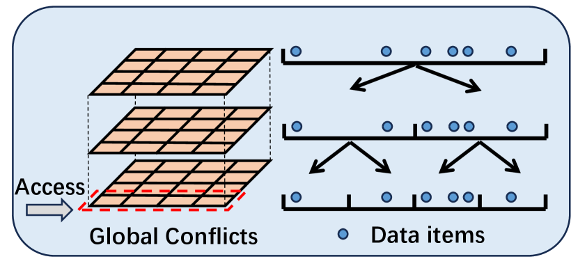
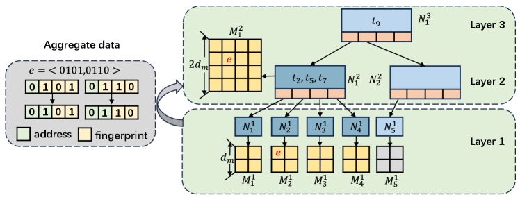
Recent advances in graph stream summarization have incorporated temporal information, targeted on supporting Temporal Range Queries (TRQ in short) [25, 6]. TRQ tasks aim to retrieve graph streams within a specified time interval, effectively answering graph queries, such as vertex, edge, path, and subgraph queries, concerning events that occurred within that time window. Horae [6] and PGSS [25] represent the latest advancements in TRQ-aided graph stream summarization, both based on TCM, with Horae achieving the state-of-the-art (SOTA) performance. Fig. 1(a) shows an example of Horae’s architecture, demonstrating top-down recursive splitting of the temporal domain into layers of uniform temporal granularities. When evaluating a vertex query within a temporal range, the query range is decomposed into multiple sub-ranges corresponding to different temporal granularities. Each sub-range necessitates a query on a specific layer. The results from these layers are then aggregated to finalize the query result. Notice that the previously mentioned multi-layer structure is not hierarchical, meaning there is no explicit parent-child relationship between layers. Then, each layer’s compressed matrix is constructed using the entire data stream on a global scale.
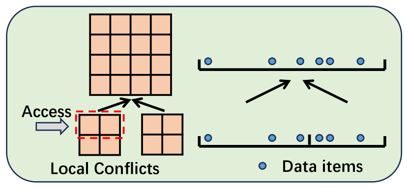
There are several drawbacks in this non-hierarchical design that have hindered the performance of graph stream summarization, in terms of query accuracy, time efficiency, and space efficiency. 1) Global Hashing Conflicts: Decomposing a query into different layers leads to global hashing conflicts at each layer, which deteriorate query accuracy. 2) Lack of Temporal Hierarchy: The absence of an explicit hierarchical structure for organizing temporal information impacts insertion and query efficiency. For example, evaluating a vertex query generates a equivalent class of sub-range queries, each requiring access to the matrix built on the global data stream and resulting in significant runtime overhead. 3) Inadaptivity to Stream Irregularity: The flat, uniform grid-like structure is not adaptive to the irregularity of graph streams. For example, there are only leaves and layers in Fig. 1(b) (bottom-up, item-based), in comparison to leaves and layers in Fig. 1(a) (top-down, domain-based). Additionally, its reliance on predefined matrix sizes undermines its adaptivity to the stream irregularity.
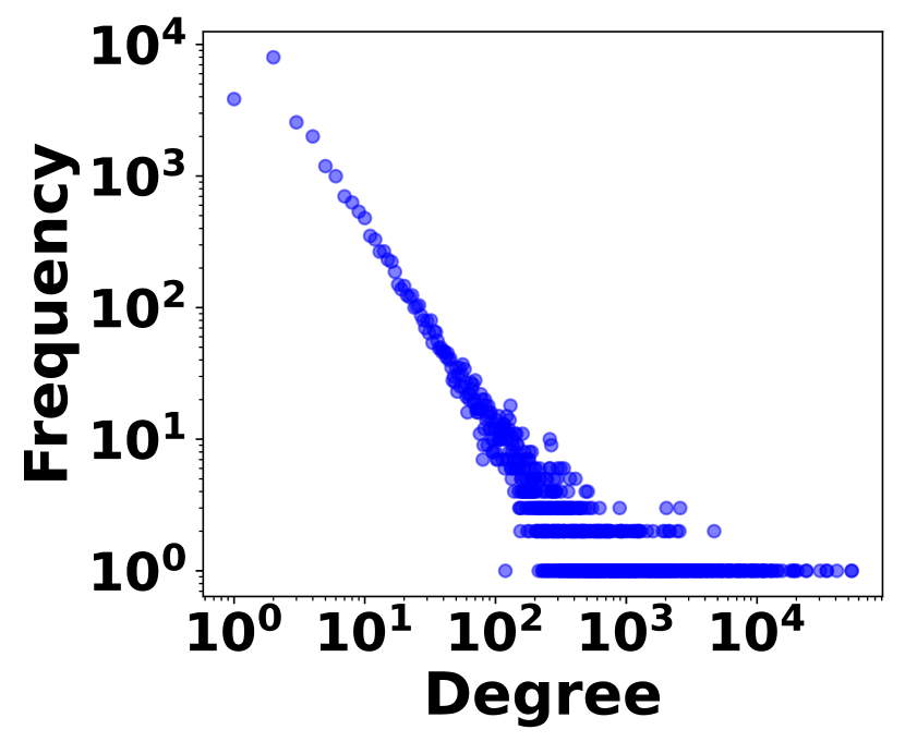
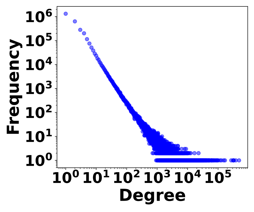
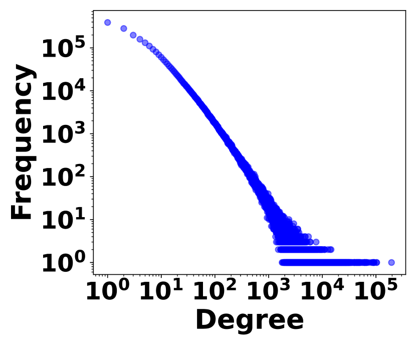
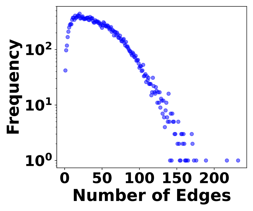
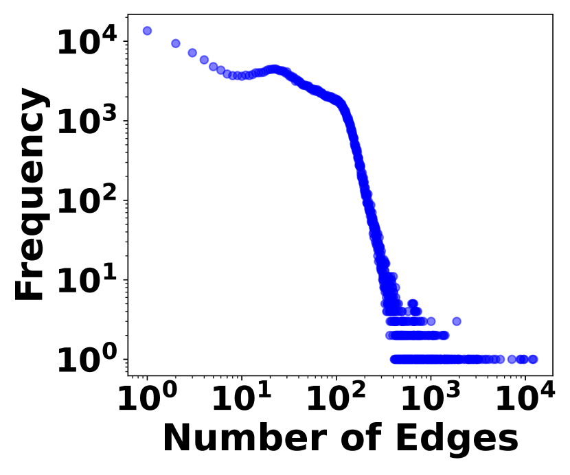
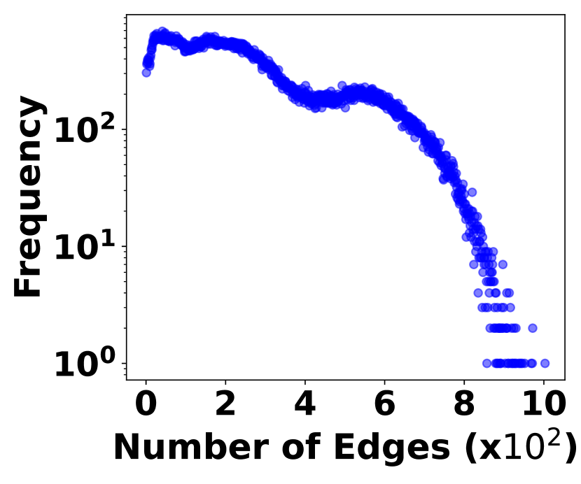
The irregularity of graph streams stems from two factors. 1) Skewed Vertex Degree Distribution: Vertex degrees follow a power-law distribution, implying a few high-degree vertices (head vertices) connect to a large number of low-degree vertices, as shown in Fig. 3. 2) Impact of Head Vertices: Changes in a head vertex lead to significant alterations in its numerous incident edges, causing substantial variations in graph streams. In Fig. 3, it shows the distribution of hot time intervals where a large number stream edges occur. The irregularity plays a crucial role in balancing space cost with query accuracy and efficiency, which is the essence of graph stream summarization.
We propose HIGGS, a novel item-based, bottom-up hierarchical data structure designed for summarizing graph streams with temporal information. HIGGS functions akin to an aggregated B-tree, as shown in Fig. 1(b), where each tree node corresponds to a specific time interval and integrates a compressed matrix representing summarized graph data from its subtree. On the bottom layer, it adaptively distributes irregular stream edges to storage buckets, optimizing space utilization and reducing the tree height. Unlike existing approaches relying on global structural information, HIGGS utilizes its hierarchical structure to localize storage and query processing and confine the changes and hash conflicts to small and managable subtrees. Moreover, HIGGS employs a meticulously designed expansion mechanism for compressed matrices, along with data aggregation and query evaluation, which not only enhance query efficiency but also ensure that no additional error is introduced during the aggregation process. As a result, HIGGS achieves significant improvements in query accuracy, as well as time and space efficiency. Additionally, we have implemented various optimizations to further enhance the performance and conducted detailed theoretical analysis to verify its advantages over existing works. Comprehensive and thorough experiments further substantiate our proposal, with results indicating that HIGGS surpasses other methods in accuracy by at least three orders of magnitude. In summary, the major contributions of this work are as follows:
-
•
We propose HIGGS, a novel item-based, bottom-up hierarchical structure designed for summarizing graph streams with temporal information. In addition, we design a expansion mechanism for compressed matrices, as well as data aggregation and query algorithms.
-
•
This structure leverages its hierarchical organization to localize storage and query processing, effectively confining changes and hash conflicts to small, manageable subtrees. By integrating data aggregation and query algorithms, it achieves significant performance improvements.
-
•
We provide a detailed theoretical analysis of our proposal, focusing on space and time efficiency, and most importantly, query accuracy, guaranteed by tighter theoretical bounds.
-
•
We report on comprehensive and thorough experiments, finding that HIGGS is capable of notable performance enhancements: it can improve accuracy by over 3 orders of magnitude, reduce space overhead by an average of 30%, increase throughput by more than 5 times, and decrease query latency by nearly 2 orders of magnitude.
| Symbol | Description |
|---|---|
| and | the number of vertices and edges in the graph stream |
| the size of the compressed matrix of the -th layer | |
| the length of the -th layer’s fingerprint | |
| the -th matrix in the -th layer | |
| the maximum number of child nodes | |
| the number of reduced fingerprint bits in aggregation | |
| the number of nodes in the -th layer | |
| the fingerprint of | |
| the address of | |
| the length of the graph stream duration | |
| the length of the time range to be queried | |
| the number of entries in a bucket | |
| the size of the value range of the hash function |
II RELATED WORK
Stream Summarization. In the era of big data, managing and analyzing massive streams of data presents significant challenges. Current solutions often rely on sketches, a set of algorithms aimed at representing large datasets with concise summaries. Extensive literature covers various sketching techniques, including Count Sketch [27], count-min (CM) sketch [26], CU sketch [28], among others [29, 30, 31, 32, 33, 34, 35, 36, 37]. For example, the CM sketch utilizes arrays of counters, each associated with a unique hash function. Upon the arrival of a stream item, each hashed counter is incremented. Deletion reverses this process by decrementing the counters. During querying, the minimum value across the hashed counters is returned for the queried item.
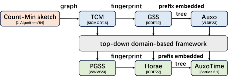
Graph Stream Summarization. Graph stream processing is inherently more complex than conventional data stream processing, due to the underlying graphical topology. As a result, considerable research has focused on graph stream summarization [23, 24, 5, 7, 6, 25, 38, 39, 40, 41, 42]. Fig. 4 shows the technical evolution of graph stream summarization. TCM, introduced by Tang et al. [23], employs multiple matrices, each associated with a hash function. During updates, these hash functions determine the insertion locations based on the hash values of the edge’s source and destination nodes, mapped to row and column addresses in the matrices. When querying, TCM retrieves the minimum aggregated weight from corresponding positions across all matrices. Despite its versatility in supporting vertex and path queries, TCM’s accuracy suffers from significant hash collisions. Addressing this issue, Khan et al. proposed gMatrix [24], a variant of TCM using reversible hash functions to enhance query support but introducing additional errors. To improve the accuracy of queries in TCM, Gou et al. proposed GSS [5], which uses a matrix and an adjacency list for data storage, employing fingerprints for edge identification. When an edge is hashed into a matrix bucket, it checks whether the fingerprints match: if yes, the weights are aggregated; otherwise, the edge is inserted into the adjacent list. To reduce the size of the list, square hashing is employed to increase edge mapping positions in the matrix, thereby reducing insertions into the list. However, handling large-scale graph streams with GSS remains challenging because the potential for high volumes can lead to longer lists, which in turn can degrade performance. Jiang et al. introduced Auxo [7], a scalable graph stream summarization method using the prefix embedded tree (PET). PET arranges compressed matrices in a tree structure and directs edge insertion based on prefix fingerprints. They also developed a proportional incremental strategy to improve PET’s memory efficiency. Consequently, Auxo exhibits good scalability with large-scale graph streams. However, like other existing methods mentioned, Auxo lacks support for temporal range queries.
Stream Summarization for TRQ. Recent advancements in supporting time range queries include many methods [43, 44, 45, 46]. Wei et al. introduced persistent CountMin and AMS sketches [43], which enable querying historical data streams. Peng et al. proposed the Persistent Bloom Filter [44], designed to identify elements within specific time intervals. Shi et al. developed at-the-time persistent (ATTP) and back-in-time persistent (BITP) sketches [45] for temporal analytics on data streams. Fan et al. enhanced temporal membership queries with the hopping sketch [46], using a sliding window approach for accurate frequency queries. However, these methods do not cater specifically to graph streams and do not preserve graph topological structures, limiting their ability to execute queries based on graph topology.
Graph Stream Summarization for TRQ. Cutting-edge works that can maintain graphical topology and support time range queries include PGSS [25] by Jia et al. and Horae [6] by Chen et al. PGSS extends TCM by storing multiple arrays of counters in each matrix bucket, each corresponding to a different time granularity. When inserting edges, it uses hash functions to locate bucket positions and updates counters based on the time granularity or layer. Horae, on the other hand, employs time prefix encoding in a multi-layer framework. Each layer operates as a GSS with specific time granularity, encoding edges upon arrival and updating nodes and time prefixes accordingly. Both PGSS and Horae adopt a top-down, temporal domain-based multi-layer approach. During queries, they decompose time ranges into sub-ranges per layer granularity, query each sub-range, and aggregate results.
However, this top-down domain-based structure struggles with irregular graph streams, resulting in poor space efficiency. Each layer employs a compressed matrix for the entire stream, leading to potential hashing conflicts and reduced accuracy. Additionally, larger matrices per layer and the need to access more buckets for time-range queries lower query efficiency.
III PROBLEM STATEMENT
Definition 1 (Graph Stream).
A graph stream is a sequence of edges arriving sequentially over time, where represents a directed edge from vertices to at time with weight .
Understanding graphical information for any temporal range is crucial, encompassing edge, vertex, path, and subgraph queries. These queries, referred to as Temporal Range Queries (TRQ in short), are essential for extracting meaningful insights and comprehending the evolving structure of the graph. Two fundamental primitives for TRQ are edge and vertex queries:
Definition 2 (TRQ Primitives).
Given a streaming graph and a temporal range , the two query primitives, node and edge queries can be defined as:
-
•
Edge Queries. Given a directed edge and a specific temporal range , the query returns the aggregated weight of this edge within .
-
•
Vertex Queries. Given a vertex and a specific temporal range , the query returns the aggregated weight of all outgoing (or incoming) edges within .
Based on the two primitives, more advanced queries, such as path and subgraph queries, can be performed to gain deeper dynamical and graphical insights. For example, in a subgraph query, we can perform an edge query for each edge within the subgraph, aggregate the weights, and return the results.
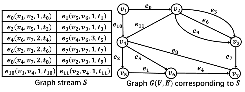
Example 1.
Fig. 5 depicts the graph stream and its associated graph . The aggregated weight of the directed edge from to is , the sum of weights at and . For vertex queries, the total weight of ’s outgoing edges from to is , calculated from the edges , , and . For the subgraph between and , only edges and contribute to the total weight of , obtained at and , respectively.
The symbols used in this paper are listed in Table I.
IV Methodology
In this section, we report technical details about the proposed item-based, bottom-up hierarchical architecture. Section IV-A illustrates the overview of the architecture. Section IV-B investigates relevant operations, including construction, insertion, and query evaluation. Section IV-C discusses the optimization techniques for further enhancing the performance.
IV-A Architecture
The architecture of HIGGS is essentially an aggregated B-tree with the following properties:
-
•
Each tree node corresponds to a time interval and is with at most children, along with a compressed matrix, summarizing the graph stream for that interval.
-
•
A non-leaf node with children contains keys, which are represented by timestamps acting as separation values dividing its subtrees. All leaves appear on the same layer, i.e., the bottom layer.
-
•
Each bucket, essentially an element in the compressed matrix, contains a set of entries, each representing the tuple for an edge .
-
–
and are fingerprints (compact identifiers) of the source and destination vertices, respectively;
-
–
is the offset relative to the matrix’s start time;
-
–
is the weight of .
-
–
Example 2.
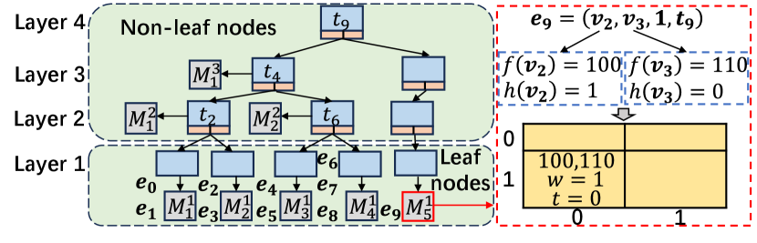
Fig.6 shows the HIGGS structure, which includes four layers: the bottom layer contains leaf nodes, and the top three layers comprise non-leaf nodes. Each node holds up to one key and can link to two children. Matrices, labeled as where is the level and the matrix number, are indexed by timestamp intervals , each covering a specific time range. For example, spans to , while covers to .
The non-leaf nodes of HIGGS, like leaf nodes, store multiple keys and pointers to compressed matrices. These keys represent the aggregated temporal scope of their child nodes. Each non-leaf node matrix summarizes data from its child nodes, devoid of timestamps, containing entries as .
IV-B Operations of HIGGS
Construction. The construction of HIGGS is item-based and bottom-up, utilizing the sequence in which graph streams arrive. When an edge arrives, it is inserted into the newest compression matrix at the first level in time. If the matrix is full, a new one is constructed to store the edge, and its timestamp is propagated upwards. If the root becomes full, a new root is created with the original one as its child. Filler nodes ensure that matrices connected to leaf nodes remain at the leaf layer, keeping the tree balanced.
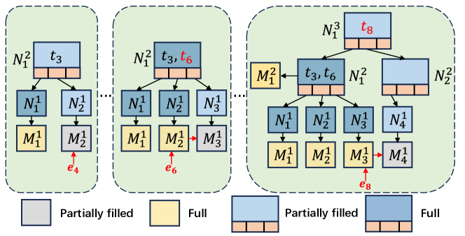
Example 3.
Fig. 7 illustrates the evolving HIGGS structure with the insertion of edge . Each node holds up to two keys and three children. Edge is smoothly inserted into matrix , whereas edge is relocated to node due to conflicts. Similarly, edge also moves to , which then reaches its capacity, therefore forming a new node to house . This causes data aggregation into matrix and the creation of empty node to link and .
Insertion. Algorithm 1 outlines the edge insertion procedure for HIGGS. Initially, HIGGS consists of a single root node, linked to an empty compression matrix . When an incoming edge arrives, it is processed using a hash function to obtain the hash values and for and , respectively. The -bit suffixes of and are then concatenated to create a fingerprint pair . The remaining bits are used to compute the address pair . For efficiency, we derive bit operations for calculating a vertex’s fingerprint and address:
| (1) |
Based on the calculated address, we can quickly locate the bucket . We then check each entry in this bucket that has a value. If an entry’s fingerprint pair matches and the recorded timestamp is , we increase its stored weight by . If no such entry is found, we insert into an empty entry. If all entries are occupied without a match, the insertion fails, prompting the creation of a new leaf node that connects to a matrix of the same size as , into which the edge is inserted in the same manner. The timestamp is then transmitted to the parent node to serve as an key during queries.
Example 4.
As shown in Fig. 6, consider the edge from Fig. 5. When insertion into fails, the timestamp propagates upward, prompting the construction of a new matrix to insert . By hashing source node and destination node , we obtain the fingerprint pair and address pair . Using the address pair, we locate bucket and insert ’s fingerprint pair, weight, and an offset of 0 relative to the matrix’s start time.
Aggregation. The aggregation between a parent node and its children plays a vital role in enhancing query accuracy and efficiency. The aggregation process follows a bottom-up way:
-
•
Leaf Nodes: Each leaf node’s compressed matrix is directly computed based on raw stream items.
-
•
Non-Leaf Nodes: Matrices of upper-level nodes aggregate those of their children, encompassing the descendant nodes within their subtrees.
Algorithm 2 describes the details of the aggregation process. For a node at the -th layer, we construct a matrix to aggregate the matrices of size from its children at the -th layer. We observe that a larger matrix increases the number of address bits. An intuitive approach is to shift additional fingerprint bits into the address, thereby reducing the storage required for fingerprints. Binary representation, which is conducive to data compression and expansion, facilitates data aggregation through simple shift operations. To avoid introducing additional errors during the aggregation process, we maintain the matrix size as a power of two. Assuming that the aggregation process reduces the fingerprint storage by bits, increasing the address bits by , the matrix size becomes times its original size. Therefore, needs to be a power of four. At the -th layer, the fingerprint length is restricted to bits. Here, denotes the maximum number of child nodes connected to a node, and and represent the matrix size and fingerprint length at the -th level, respectively. It is noteworthy that the aggregation operation does not involve the storage of timestamps.
Example 5.
Fig. 8 shows an example of data aggregation with , , and . For edge in , its address pair is and fingerprint pair . During aggregation to , with , the leftmost bit of the fingerprint moves to the address’s rightmost bit. The new address pair locates in , where fingerprint pair is stored.
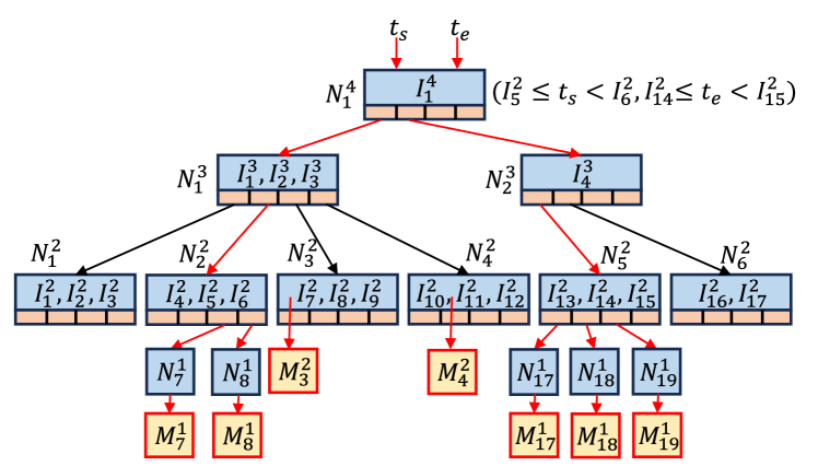
TRQ Evaluation Framework. For any specified temporal range query, including edge, vertex, path, and subgraph queries, it can be broken down into a series of sub-range queries using the boundary search algorithm (Algorithm 3) run on HIGGS. Each sub-range query is performed on its respective compressed matrix, thereby transforming the problem into querying across a set of matrices. Different types of query primitives, such as edge and vertex queries, correspond to different methods of accessing the compressed matrices. The boundary search algorithm involves two main steps:
First, starting from the root node of HIGGS, the algorithm identifies the child nodes entirely covered by the queried range and adds them to the query list . If falls within the range represented by a child node, further queries are made into the child node, continuing until and no longer reside within the range of the same child node.
Second, the algorithm then identifies the child nodes containing or and adds the child nodes of parent nodes that are contained by or to . If or exactly matches the start or end point of a node’s range, the corresponding query can be directly terminated; otherwise, the search extends to the next level of child nodes containing or . Upon reaching the leaf nodes, in addition to adding nodes that meet the previously mentioned conditions, nodes containing or are also added to . This concludes the decomposition process of the temporal range.
Example 6.
Fig. 9 illustrates how a boundary search algorithm decomposes a range within a four-level HIGGS structure (). For time range , starting from , the search proceeds to nodes (containing ) and (containing ). Since no child nodes are fully within , children of (, ) and child of are queried and added to list . Leaf node , containing , is also added. The process is mirrored for , resulting in query list containing matrices , and .
Next, we proceed to discuss how the query framework is implemented for TRQ primitives, i.e., edge and vertex queries.
Edge Queries. For a temporal query range , an edge query from to is conducted on matrix . Using Formula (1) and a shift operation, we derive the fingerprint and address , locating the bucket .
Two cases arise: 1) Non-leaf node: If is a non-leaf, we check if any entry’s fingerprint matches —if so, return its weight; otherwise, it returns . 2) Leaf node: If is a leaf, we additionally check if the timestamp falls within . If both the fingerprint and timestamp match, the entry is considered valid, and we proceed as in the non-leaf case.
Vertex Queries. For the temporal query range , queries are made on a source or destination vertex based on matrix of size . Using Formula (1) and a shift operation, we ascertain ’s fingerprint and address , then locate the corresponding row in :
| (2) |
Each entry in the row’s buckets is traversed. For non-leaf nodes, if the source vertex’s fingerprint matches , the weight is added to the result. For leaf nodes, both the fingerprint must match and the timestamp must fall within for the weight to be included.
IV-C Optimization
We propose three optimizations: multiple mapping buckets to enhance space efficiency, overflow blocks to improve accuracy, and parallelization to boost insertion throughput.
Multiple Mapping Buckets (MMB). When inserting an edge , using only a single mapping bucket can lead to severe conflicts, potentially causing the insertion to fail and wasting significant space if the matrix is underutilized. To address this issue, we employ multiple mapping buckets, giving each edge multiple potential insertion positions. Specifically, we use the linear congruence method [47] to generate address sequences for the source vertex and for the destination vertex , where represents the number of mapping positions of a vertex. The address sequences of the source and destination vertices are then combined pairwise to produce mapping buckets. To track the position of each bucket in the address sequence, we record an index pair . In this way, insertion only fails if all mapping buckets conflict, significantly reducing the likelihood of failure and improving space utilization of the matrix.
Overflow Blocks (OB). In the basic HIGGS framework, if an edge insertion at a leaf node fails, a new leaf is created to store the edge, and its timestamp is transmitted to the parent as a key to distinguish between leaf nodes. However, if multiple edges with identical timestamps have already been stored, this key becomes ineffective, leading to errors. To resolve this, we employ overflow blocks to aggregate edges that arrive simultaneously into a unified time range. If an edge insertion fails and has the same timestamp as the previous edge, an overflow block is created on the current leaf to store it; otherwise, a new leaf is created. The overflow block is essentially a small-scale compressed matrix, enabling more precise partitioning of the graph stream by timestamps and thereby enhancing query accuracy.
Parallelization. To enhance throughput, we adopt a parallel updating strategy, assigning each layer a separate thread that updates only the latest node. To maintain data consistency across the subtree, each element is first updated by the thread corresponding to leaf nodes before being processed by other threads. Since order preservation is needed only at the element level, parallel efficiency remains high. By utilizing parallelism, the throughput of HIGGS is increased substantially.
V ANALYSIS
V-A Space Cost Analysis
Space Savings through Aggregation. Compared to the storage methods employed in existing works, our design significantly reduces space costs.
Theorem 1.
Compared to the storage methods of the existing proposals, a HIGGS structure with layers reduces the space cost by a proportion of , where denotes the size of each entry within the matrix.
Proof.
Consider a HIGGS structure with leaf nodes, each with a compressed matrix. For simplicity, we assume that is divisible by . In this setting, using the storage method of the previous framework, the space consumed is:
| (3) |
Through the aggregation of matrices and the compression of fingerprints, the saved space is:
| (4) |
Thus, the ratio of space saved is:
| (5) |
Thus, the theorem is proven. ∎
Matrix Utilization Rate. The utilization rate of a matrix refers to the proportion of elements stored within the matrix relative to its total capacity. As discussed in Section IV-C, for a compressed matrix, we enhance the utilization rate of the bucket by setting the number of mapping buckets for each edge to . Simultaneously, each bucket contains entries. An insertion failure indicates that all mapping buckets have encountered conflicts, while all previous edges were successfully inserted. Let denote the probability that -th edge is inserted successfully, and represent the probability of its failure. If -th edge causes the first insertion failure, the probability of this occurrence, according to the geometric distribution, is:
| (6) | ||||
Given that the compressed matrix containing elements, the expected utilization of the matrix is calculated as follows:
| (7) |
Here, represents the expected number of elements successfully inserted into the matrix. Therefore, the formula quantifies the average utilization of the storage block by considering the successful insertions relative to the total number of available elements of its associated compressed matrix.
Space Complexity Analysis. The number of layers in HIGGS primarily depends on the quantity of leaf nodes and the out-degree of each node. Since the space occupied by a compressed matrix to which a non-leaf node points equals the cumulative space of the matrices of all its corresponding child nodes, the space overhead for each layer in HIGGS is fundamentally consistent. Let the average space utilization rate of each matrix pointed to by the leaf nodes be , and let the space occupied by the keys in HIGGS be . The number of matrices at the leaf nodes is given by , leading to a space complexity for HIGGS of approximately . Since the space required for storing keys is significantly less than that needed for storing graph stream data, the overall space cost is . After optimization with overflow blocks, assuming the average time span represented by each matrix is (where ), the formula can be derived as follows:
| (8) |
represents the space complexity of the existing framework. This establishes that the space complexity of HIGGS is superior to that of the existing framework. Additionally, the fewer edges arrive per unit time in the graph stream, that is, the larger the value of , the lower the space cost becomes.
V-B Query Efficiency Analysis
The time complexity of HIGGS depends on the number of matrices accessed at each layer. Assuming the length of a given temporal range query is , at most matrices are queried, leading to a time complexity approximates O().
Furthermore, the query at each layer in the existing framework targets the data structure that stores the entire graph stream, resulting in larger scales. Consequently, when addressing temporal range queries related to topological structures, this framework accesses a greater number of buckets, which leads to lower query efficiency. In contrast, the total size of all matrices to be queried in HIGGS is consistent with the size of the graph stream within that time range, making it smaller in scale and more efficient to access.
V-C Scalability Analysis
As streaming edges continuously arrive, HIGGS increases the number of leaf nodes to store data while aggregating at non-leaf nodes. The number of layers in HIGGS is , with a space complexity of , an update time complexity of , and a query time complexity of , where is the number of leaf nodes, is the query range length, and is the average time range length represented by each leaf node. To accelerate updates, we employ parallel optimization (see Section IV-C), where each layer is assigned a dedicated thread.
V-D Query Accuracy Analysis
Collision Rate Analysis. In this section, we analyze the collision rates for nodes and edges maintained in HIGGS. Moreover, we show that HIGGS has one-sided error, i.e., it only overestimates the true query results; it never underestimates results.
1) Node Collision. For a given temporal query range and an edge , conflicts for ’s source (or destination) node arise only from other edges within this time range. Specifically, if there exists an edge conflicting with , the following conditions must be met:
-
•
(or );
-
•
(or );
-
•
.
Suppose that within the time range , the number of source (or destination) nodes different from (or ) is denoted as . The total number of distinct source (or destination) nodes in the entire graph stream is , and the size of the value range of the hash function is , where . The probability of a node conflicting with is . Given that there are such nodes within , the node conflict probability for is,
| (9) | ||||
From the equation, it is evident that increasing the number of fingerprint bits or the size of the compression matrix in the first layer will reduce the probability of node conflicts.
2) Edge Collision. Similar to node collision, when provided with a specified time range and an edge for a query, edges outside beyond the time range will not conflict with . If there is an edge that conflicts with , it must satisfy the following conditions:
-
•
or
-
•
and
-
•
Then, the collision probability of edge is:
| (10) | ||||
Here, denotes the number of edges that, within the range , share the same source or destination node as and have a probability of conflict with of . Conversely, the probability of conflict for the remaining edges, which are distinct from , is . Additionally, denotes the number of edges distinct from within this range. and respectively signify the maximum out-degree and in-degree across the entire graph stream, while denotes the count of distinct edges throughout the graph stream. Similar to node collision, increasing the fingerprint size or matrix size in the first layer proves effective in reducing the probability of conflicts.
Error Bounds. Next, we analyze the error bounds for node and edge queries in HIGGS and the configuration of the fingerprint length and the matrix size of the leaf nodes.
1) Error Bound for Vertex Queries. We use and to represent the estimated value and the actual value for vertex queries within the range of length , respectively. Given a parameter , we set , resulting in . We denote the number of edges within the range as and the sum of their weights as .
Theorem 2.
The result has the guarantee: with a probability of at least .
Proof.
Consider two edges, and , within the same time range . We introduce an indicator which is one if there is a source node collision between the two edges, and zero otherwise. We can have the expectation of as follows.
| (11) |
Let denote . Then, it follows that:. By linear expectation,
| (12) | ||||
By applying the Markov inequality, we have:
| (13) | ||||
Thus, Theorem 2 is proven. The destination vertex query can be analyzed in a similar way. ∎
2) Error Bound for Edge Queries. Similar to vertex queries, We use and to respectively denote the estimated value and the actual value for edge queries within the range of length .
Theorem 3.
The result guarantees with a probability of at least .
Proof.
Consider two edges, and , within the same time range . We introduce an indicator , which is 1 if there is an edge collision between the two edges, and is 0, otherwise. We then have the expectation of :
| (14) | ||||
Let denote . By construction, . By linear expectation, we have:
| (15) | ||||
By applying the Markov inequality, we have:
| (16) | ||||
Thus, Theorem 3 is proven. ∎
VI EXPERIMENTAL STUDY
We have implemented HIGGS and made the code available as open source on GitHub111https://anonymous.4open.science/r/HIGGS-1215/. We report on experiments with HIGGS on real-world graph streams to answer the following research questions.
-
Q1.
Can HIGGS outperform SOTA methods, including PGSS, Horae, Horae-cpt, AuxoTime, and AuxoTime-cpt, in terms of the query accuracy, efficiency, and scalability, for different types of graph queries, including edge, node, subgraph, and path queries?
-
Q2.
What is the space overhead, deletion throughout, insertion throughput and latency of all competitors in achieving the query performance as aforementioned?
-
Q3.
What is the effect of proposed optimization techniques, such as multiple mapping buckets, parallelization, and overflow blocks, particularly concerning space overhead, throughput and accuracy, respectively?
VI-A Experimental Setup
Baselines. In the field of graph stream summarization supporting temporal range queries, SOTA methods include PGSS and Horae, with Horae excelling in query accuracy. However, their scalability is limited. Therefore, we create stronger baselines by extending the SOTA graph stream summarization structure, i.e., Auxo, to support temporal range queries through the incorporation of Horae’s range decomposition scheme, yielding AuxoTime. Additionally, Horae has an optimized variant, Horae-cpt, aimed at reducing space overhead, which prompted us to also develop AuxoTime-cpt. In the empirical study, we consider five competitive baselines, including PGSS, Horae, Horae-cpt, AuxoTime, and AuxoTime-cpt.
| Dataset | Nodes | Edges | Time Span | Time Slice |
|---|---|---|---|---|
| Lkml | 63,399 | 1,096,440 | 2006-2013 | 1 second |
| Wikipedia talk | 2,987,535 | 24,981,163 | 2001-2015 | 1 second |
| Stackoverflow | 2,601,977 | 63,497,050 | 2009-2016 | 1 second |
Datasets. We consider 3 real datasets commonly used for evaluating graph stream summarization, namely Lkml, Wiki-talk, and Stackoverflow, as shown in Table II. The Lkml dataset [48] is a communication network of the Linux kernel mailing list, where nodes represent users (email addresses) and directed edges denote replies, encompassing 63,399 users and 1,096,440 replies. The Wikipedia talk (WT in short) [48] dataset captures the communication network of the English Wikipedia, with nodes representing users and edges indicating messages written on other users’ talk pages, comprising 2,987,535 nodes and 24,981,163 messages. The Stackoverflow (SO in short) [48] dataset, collected from 2009 to 2016, represents an interaction network between users on Stack Overflow, featuring 2,601,977 nodes and 63,497,050 edges222The time slice for each dataset is set to 1 second to align with the time unit settings of each dataset..
Metrics. The metrics primarily include average absolute error (AAE), average relative error (ARE), average query time, throughput, and space cost. AAE and ARE are commonly used for evaluating the accuracy of graph summarization, quantifying the error between the true values and the queried values. If there are queries, each with a true value and an estimated value , then:
| (17) |
Average query time reflects the system’s performance on average query response for a series of query operations. Insertion throughput measures the number of elements processed per unit time, while insertion latency indicates the speed of processing insertions. Space overhead indicates the amount of main memory required to store or process data in the system.
Configuration. Experiments were done on a machine equipped with a 32-core 2.6 GHz Xeon CPU, 384 GB RAM, and a 960 GB SSD. Baseline parameters were set following corresponding papers. For HIGGS, we set the number of optional addresses for each node to and to . Therefore, for each edge, bits are required to store the index pair, indicating the position. Due to the close correlation between and the degree of conflicts, we configured parameter to and to to ensure that the value of HIGGS aligns with those of the baselines. For vertex and edge queries, we vary the query range length from to . For each , we randomly generated 100K edge queries and 10K vertex queries. For path and subgraph queries, the path length is set to and subgraph size is set to . For each path length and subgraph size, 1K queries are randomly generated. Each value reported is the average of 1,000 runs.
VI-B Performance on Edge and Vertex Queries
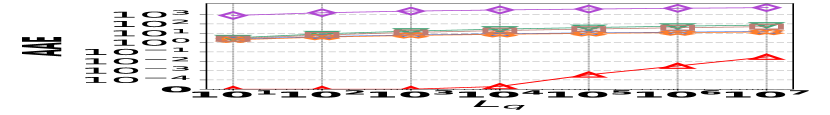
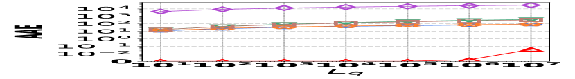
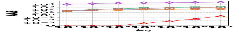
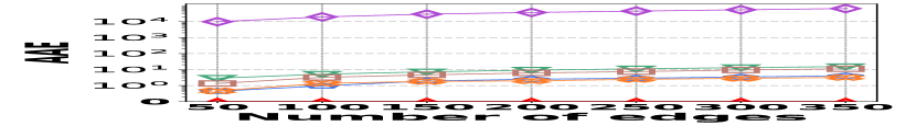
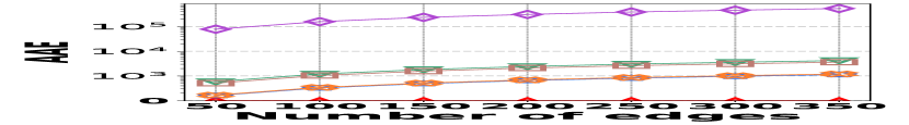
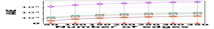
1) AAE vs. L: Fig. 15 (a–c) examine the accuracy of edge queries for all competitors in terms of AAE. In all experiments, the AAE of HIGGS is notably lower than those of other baselines, and this is consistent across all the three real graph stream datasets, i.e., Lkml, Wikipedia talk, and StackOverflow. For example, when the length of the query range equals , the AAE of HIGGS is about orders of magnitude lower than that of the second-best competitor on Stackoverflow (Fig. 10(c)). Remarkably, the AAE of HIGGS is almost zero on the Lkml dataset (Fig. 10(a)), implying 100% query accuracy. The superior performance of HIGGS is attributed to the elimination of conflicts of streaming items in the upper layers. In contrast, other methodologies experience an accumulation of errors as the query range expands, resulting in inaccuracies caused by the error accumulation in the query processing. Since the number of structure layers and the length of the query range are logarithmically related, the AAE of these methods increases logarithmically as the query range expands. However, our approach avoids the inter-layer error accumulation. Even when the temporal range spans the entire graph stream, the conflicts in HIGGS are confined to the layer of leaf nodes. This also explains why, when the query range is exceptionally large, the advantage of HIGGS over other competitors becomes smaller, since the task of TRQ degenerates into the task of count estimations of conventional (non-temporal) graph summaries like TCM. Although the accuracy of HIGGS is slightly lower, it remains orders of magnitude better than the accuracies of its competitors. Furthermore, the AAE of Horae-cpt and AuxoTime-cpt are higher than those of Horae and AuxoTime, respectively, as they decompose the temporal query range into more sub-ranges, leading to increased query conflicts and, consequently, a relative increase in AAE.
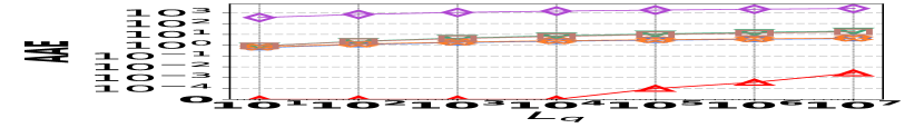
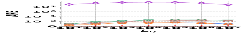
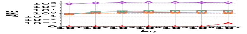
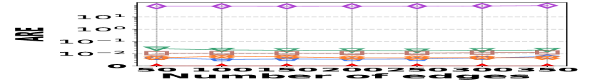
2) ARE vs. L: Fig. 15 (d–f) depict the ARE results for edge queries across three datasets, as the query range length varies. Similar to the result observed in Fig. 15 (a–c), HIGGS consistently outperforms other baselines and maintains near-lossless performance across all three datasets, showcasing its advantage. It is noteworthy that in Fig. 15 (d–f), the ARE of the baselines initially increase and then decrease. This pattern is due to the relative error decreasing as the true edge weights increase with the lengthening of the query range.
![[Uncaptioned image]](https://cdn.awesomepapers.org/papers/381ce240-522c-4b11-a9c7-59ac8f25ada9/x15.png)
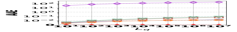
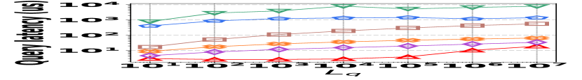
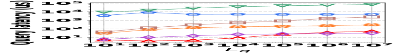
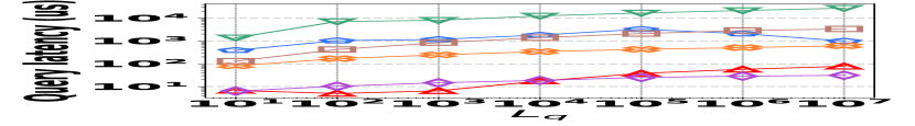

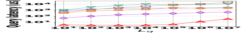
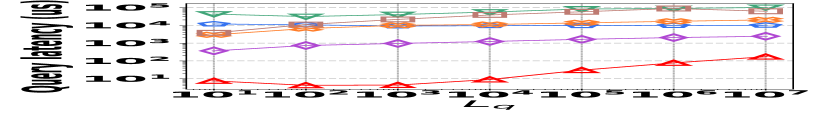
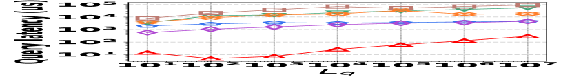
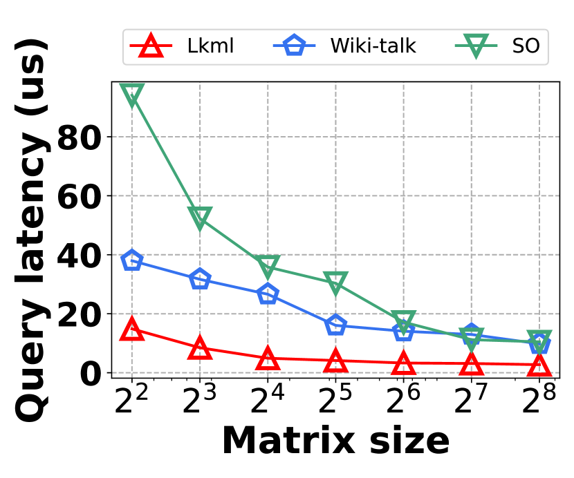
3) Latency vs. L: Fig. 15 (g–i) illustrate the relationship between the query latency and the length of the query range, across all datasets. It shows that HIGGS and PGSS markedly outperform other baselines: when the query range length is set to , HIGGS surpasses AuxoTime by an order of magnitude and improves on Horae by two orders of magnitude. The superior performance of HIGGS stems primarily from its ability to access fewer summary layers given the same query range, and each layer accesses fewer nodes/buckets compared to AuxoTime and Horae. PGSS exhibits competitive query latency (Fig. 15(g–i)), but it falls short in query accuracy (Fig. 15(a–f)). Additionally, Horae’s query efficiency is compromised by excessive accesses to the buffer structure, degrading its performance, as is the case with AuxoTime. Moreover, the query latency of AuxoTime-cpt and Horae-cpt exceed those of AuxoTime and Horae, respectively, because they decompose the query range into more sub-ranges, increasing the query complexity from to .
The performance of vertex queries is reported in Fig. 15, where the trend is similar to that of edge queries. The details are thus omitted for brevity.
![[Uncaptioned image]](https://cdn.awesomepapers.org/papers/381ce240-522c-4b11-a9c7-59ac8f25ada9/x60.png)
Throughput
Latency
Throughput
VI-C Performance on Path and Subgraph Queries
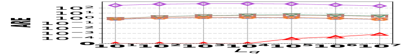
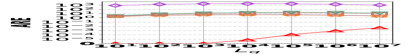
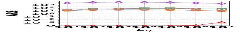
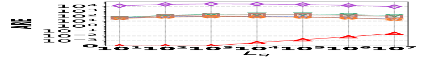
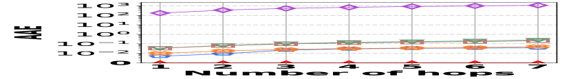
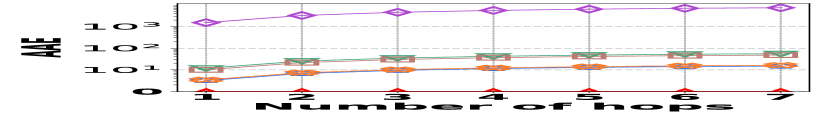
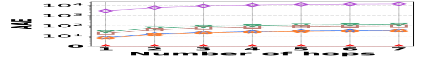
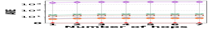
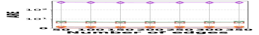
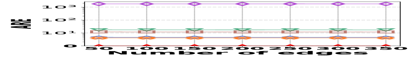
1) AAE vs. L: Fig. 15 (a–c) report the performance on path queries, in particular, the relation between the accuracy (AAE) and the path length (number of hops), with the temporal range set to . Compared to its competitors, HIGGS exhibits near-lossless performance across all three datasets, showing a clear advantage that grows with the number of hops in the path. This is due to HIGGS’s cumulative precision benefits in edge queries, which are amplified in path queries since each path query consists of multiple edge queries. Additionally, Horae and AuxoTime demonstrate similar AAE, each outperforming their respective variants, Horae-cpt and AuxoTime-cpt. The absence of fingerprint utilization in PGSS for identifying stored edges leads to significant conflicts and a noticeable decrease in accuracy.
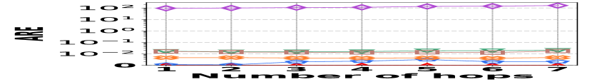
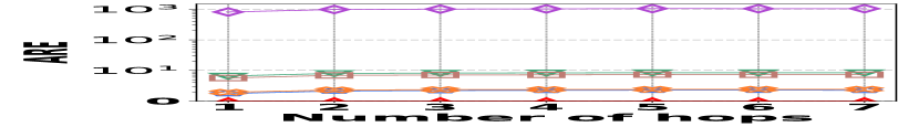
2) ARE vs. L: Fig. 15 (d–f) show the trends of the values of ARE for path queries across three datasets as the number of hops increases, with the temporal range set to . Consistent with the AAE trend, HIGGS maintains near 100% query accuracy, significantly outperforming the competitors.
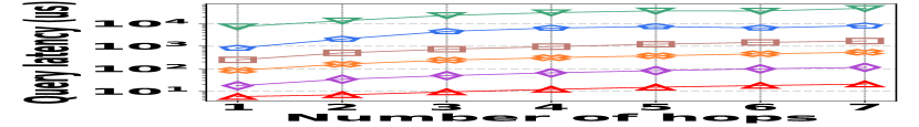
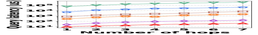
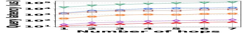
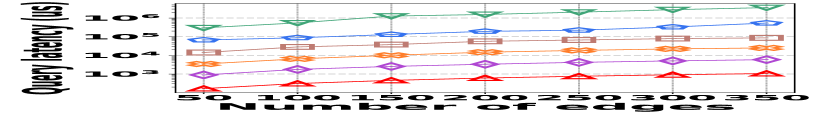
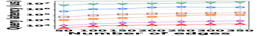
3) Latency vs. L: Fig. 15 (g–i) depict a comparative latency analysis of path queries among all the competitors and datasets. HIGGS consistently leads, e.g., on Stackoverflow, it outperforms PGSS by 2.2x, AuxoTime by 30.8x, and Horae by two orders of magnitude when the path is 4 hops. The latency disadvantages of Horae-cpt and AuxoTime-cpt in edge querying are magnified here.
Fig. 15 reports the performance on subgraph queries, including the accuracy (AAE&ARE) and query latency. The results are quite similar to that on path queries, and are omitted due to page limits.
VI-D Performance on Graph Stream Irregularity
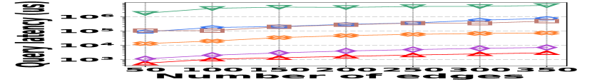
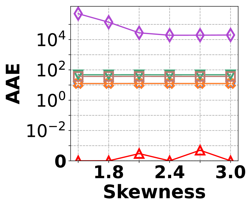
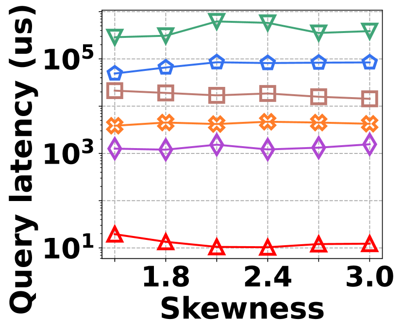
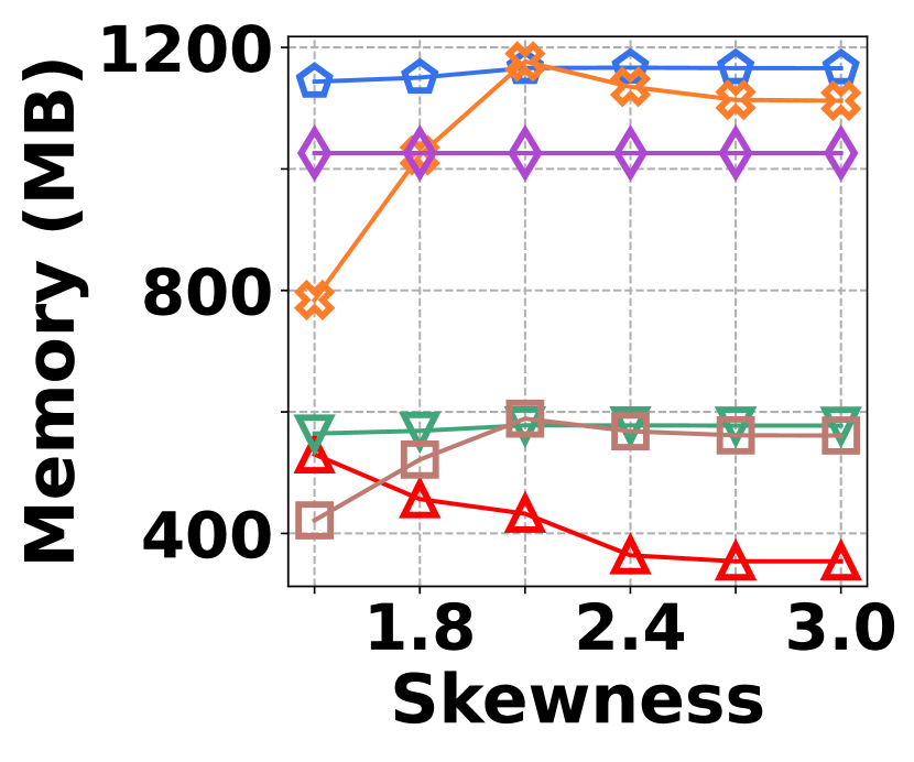
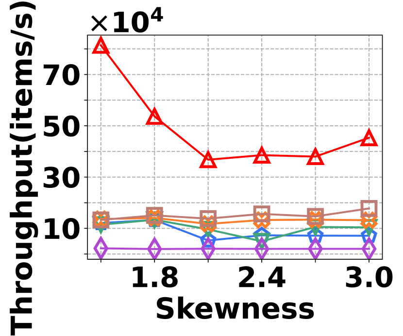
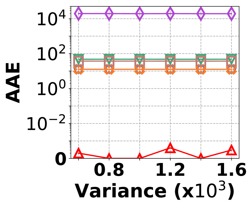
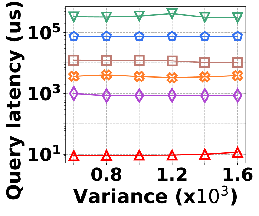
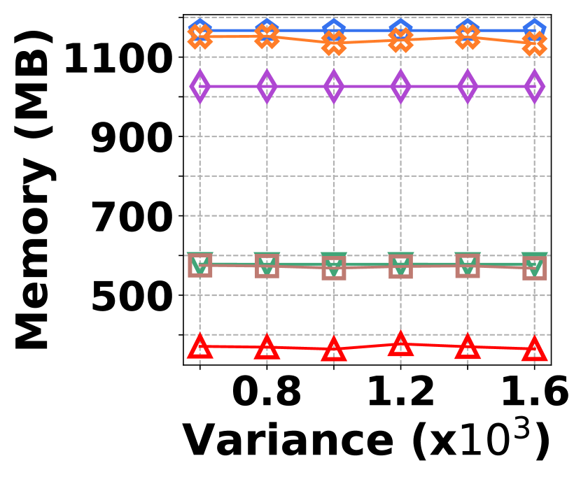
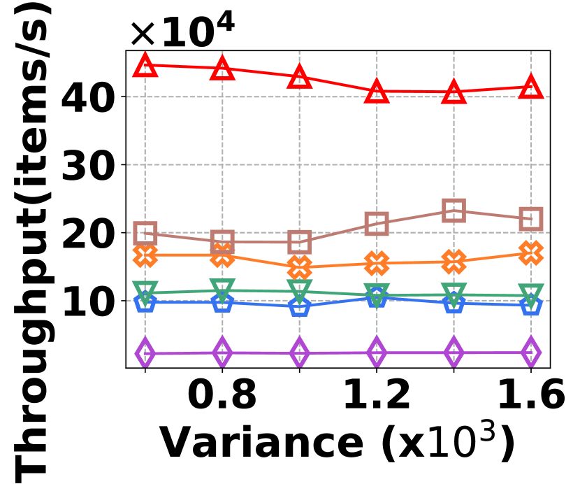
The irregularity in graph streams arises from skewed vertex degree distributions (skewness) and imbalanced edge arrivals (variance)333We synthesize 6 datasets with varied skewness indicated by power-law exponents ranging from 1.5 to 3.0, and 6 datasets with varied variances from 600 to 1,600. Each dataset contains 100K nodes and 5M edges.. Fig. 15 presents the results of vertex queries and update cost under varied skewness. HIGGS significantly outperforms other baselines in AAE, achieving zero error at a skewness of 2.4, while the best alternative has an AAE of around 10. For query latency, HIGGS leads by approximately two orders of magnitude over the runner-up. Regarding space overhead and throughput at a skewness of 2.4, HIGGS exceeds Horae by 3.2 and 5.3 times, Horae-cpt by 1.6 and 7.8 times, Auxo by 3.1 and 2.9 times, Auxo-cpt by 1.6 and 2.5 times, and PGSS by 2.8 and 19.2 times. Fig. 15 shows the performance under different variances, with HIGGS still far ahead. Due to the page limitation, further details are omitted.
VI-E Performance on Insertion Throughput and Latency
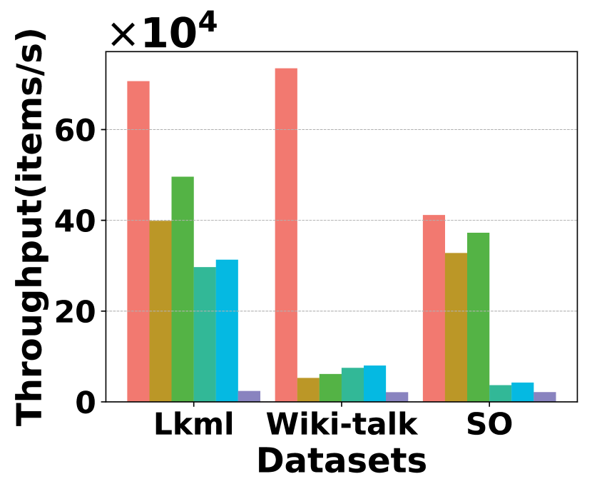
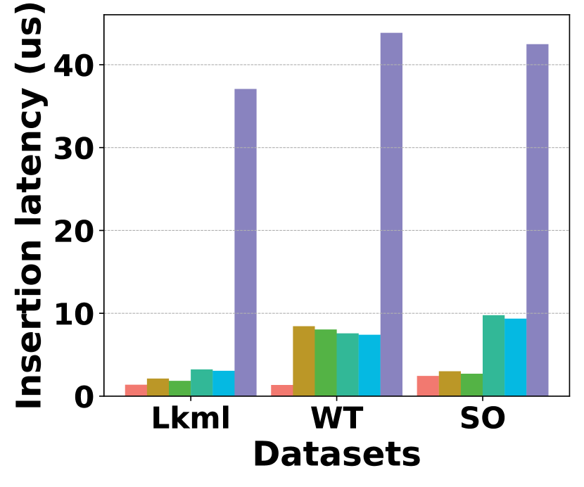
Fig. 20 compares the performance of insertion throughput for different methods on different datasets. HIGGS continues to hold a substantial lead, significantly outperforming all competitors. In particular, on Stackoverflow, it leads Horae, AuxoTime, Horae-cpt, AuxoTime-cpt, and PGSS by 1.3x, 11.2x, 1.1x, 9.7x, and 19.3x, respectively. Additionally, Horae-cpt and AuxoTime-cpt achieve slightly higher throughput compared to Horae and AuxoTime, because they store less data except the bottom layer, thus requiring fewer updates to stream item insertion. Fig. 20 presents a comparison of insertion latency among different methods. HIGGS outperforms Horae, Horae-cpt, AuxoTime, AuxoTime-cpt, and PGSS on Stackoverflow by 1.2x, 1.1x, 4.0x, 3.8x, and 17.4x, respectively.
VI-F Performance on Deletion Throughput
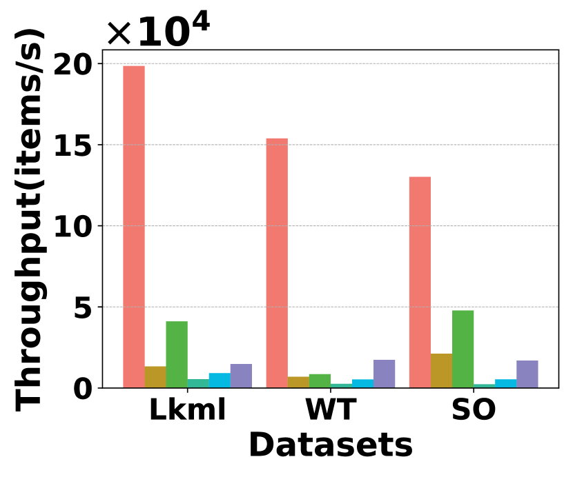
Fig. 20 illustrates the deletion throughput performance across three datasets, where HIGGS consistently outperforms other baselines. On Stack Overflow, HIGGS is faster than Horae by 6.1x, Horae-cpt by 2.7x, AuxoTime by 56.0x, AuxoTime-cpt by 24.3x, and PGSS by 7.7x.
VI-G Performance on Space Cost
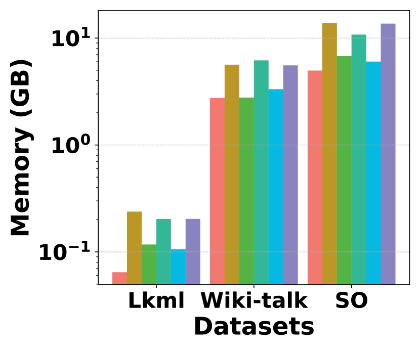
Fig. 20 presents the space overhead for different methods across different datasets. It shows that HIGGS consistently achieves the lowest space overhead on all datasets. Specifically, on Stackoverflow, it achieves a space savings of 26.8% compared to Horae-cpt, 17.5% compared to AuxoTime-cpt, 64.1% over Horae, 53.9% against AuxoTime, and 63.6% compared to PGSS. This implies that HIGGS uses less space to achieve markedly better query performance.
VI-H Optimization
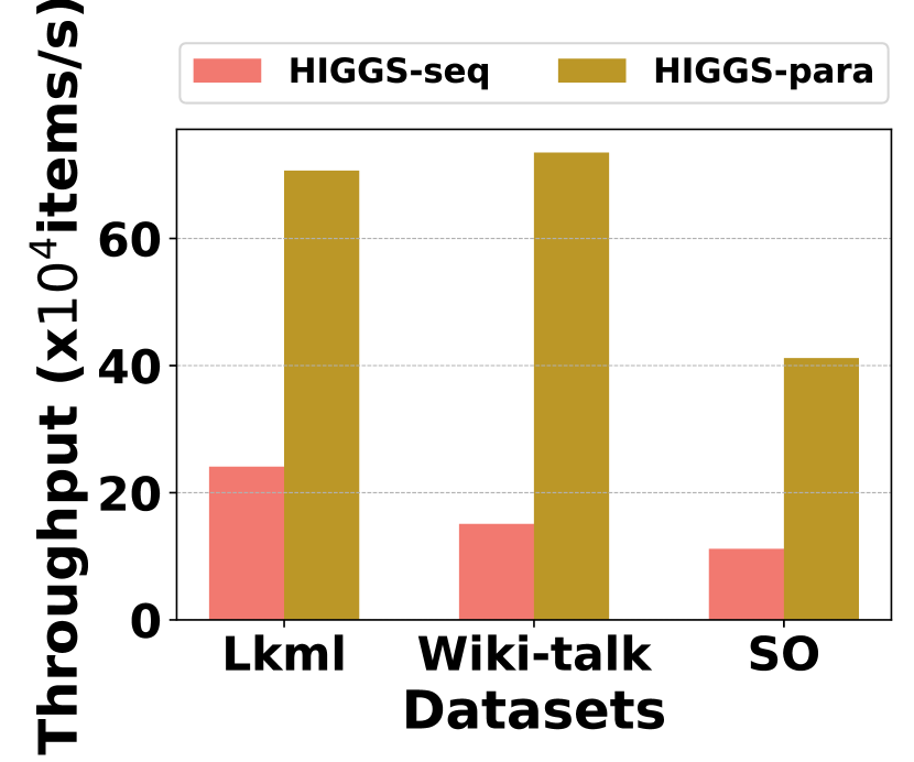
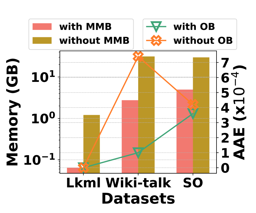
Fig. 20 evaluates the effectiveness of proposed optimizations of parallelization, multiple mapping buckets (MMB), and overflow buckets (OB). Fig. 20 (a) shows the throughput of HIGGS with and without the parallelization optimization across three datasets, where HIGGS’s throughput has increased at least 3x by adopting parallelization. In Fig. 20 (b), it shows that employing MMB substantially improves space efficiency and incorporating OB improves accuracy. For example, on StackOverflow, the MMB mechanism brings in about 6x increase in space efficiency compared to its absence, while the OB mechanism leads to a 14.3% improvement in accuracy.
VI-I Parameters
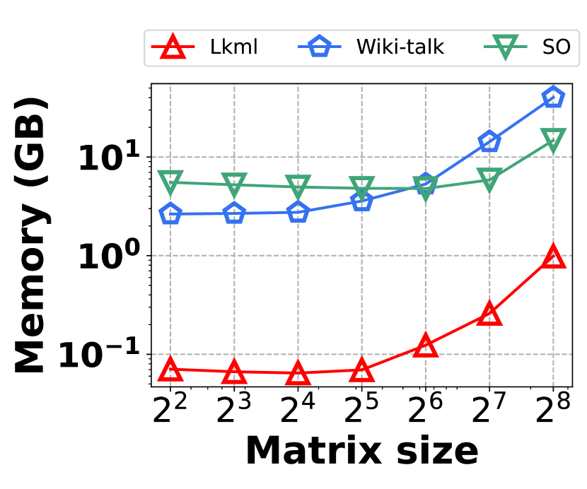
Fig. 21(b) investigates the impact of parameters about matrix size at leaf nodes on space overhead and query latency. The results demonstrate that typically, larger matrices at the leaf nodes lead to higher space cost but reduced query latency. For instance, with a matrix size of 16, the space overhead on Stackoverflow is 5,085MB, and the query latency is 35.8 s, which is significantly outperforming other competitors. Therefore, we recommend setting to 16 to achieve a good balance between the space overhead and query latency.
VII Conclusion
We propose HIGGS, a novel item-based, bottom-up hierarchical structure designed for summarizing graph streams with temporal information. HIGGS leverages its hierarchical design to localize storage and query processing, effectively confining changes and hash conflicts within smaller, manageable sub-trees. Compared to existing approaches, HIGGS achieves a notable enhancement in overall performance, supported by both a theoretical analysis and empirical studies. Extensive experiments on real graph streams show that HIGGS can improve accuracy by more than orders of magnitude, reduce space overhead by an average of %, increase throughput by + times, and reduce query response time by nearly orders of magnitude. In future research, it is of interest to extend HIGGS to support advanced graph stream variants, including foundational variants like heterogeneous graph streams with diverse node and edge types, as well as application-specific variants such as spatiotemporal, web, and social graph streams.
Acknowledgments
This work was supported by the NSFC under Grants 62472400 and 62072428. Xike Xie is the corresponding author.
References
- [1] R. Sarmento, M. Oliveira, M. Cordeiro, S. Tabassum, and J. Gama, “Social network analysis in streaming call graphs,” Big data analysis: new algorithms for a new society, pp. 239–261, 2016.
- [2] C. Aggarwal and K. Subbian, “Evolutionary network analysis: A survey,” ACM Computing Surveys, vol. 47, no. 1, pp. 1–36, 2014.
- [3] R. Long, H. Wang, Y. Chen, O. Jin, and Y. Yu, “Towards effective event detection, tracking and summarization on microblog data,” in International Conference on Web Age Information Management, 2011, pp. 652–663.
- [4] M. Cordeiro and J. Gama, “Online social networks event detection: a survey,” Solving Large Scale Learning Tasks. Challenges and Algorithms: Essays Dedicated to Katharina Morik on the Occasion of Her 60th Birthday, pp. 1–41, 2016.
- [5] X. Gou, L. Zou, C. Zhao, and T. Yang, “Fast and accurate graph stream summarization,” in International Conference on Data Engineering, 2019, pp. 1118–1129.
- [6] M. Chen, R. Zhou, H. Chen, J. Xiao, H. Jin, and B. Li, “Horae: A graph stream summarization structure for efficient temporal range query,” in International Conference on Data Engineering, 2022, pp. 2792–2804.
- [7] Z. Jiang, H. Chen, and H. Jin, “Auxo: A scalable and efficient graph stream summarization structure,” Proceedings of the VLDB Endowment, vol. 16, no. 6, pp. 1386–1398, 2023.
- [8] X. Ke, A. Khan, and F. Bonchi, “Multi-relation graph summarization,” ACM Transactions on Knowledge Discovery from Data, vol. 16, no. 5, pp. 1–30, 2022.
- [9] Z. Tian, Y. Liu, J. Sun, Y. Jiang, and M. Zhu, “Exploiting group information for personalized recommendation with graph neural networks,” ACM Transactions on Information Systems, vol. 40, no. 2, pp. 1–23, 2021.
- [10] H. Ficel, M. R. Haddad, and H. B. Zghal, “A graph-based recommendation approach for highly interactive platforms,” Expert Systems with Applications, vol. 185, p. 115555, 2021.
- [11] M. M. Gaber, A. Zaslavsky, and S. Krishnaswamy, “Mining data streams: a review,” ACM SIGMOD Record, vol. 34, no. 2, pp. 18–26, 2005.
- [12] Z. Fang, L. Pan, L. Chen, Y. Du, and Y. Gao, “MDTP: A multi-source deep traffic prediction framework over spatio-temporal trajectory data,” Proceedings of the VLDB Endowment, vol. 14, no. 8, pp. 1289–1297, 2021.
- [13] X. Gou and L. Zou, “Sliding window-based approximate triangle counting over streaming graphs with duplicate edges,” in International Conference on Management of Data, 2021, pp. 645–657.
- [14] Y. Li, L. Zou, M. T. Özsu, and D. Zhao, “Time constrained continuous subgraph search over streaming graphs,” in International Conference on Data Engineering, 2019, pp. 1082–1093.
- [15] A. Pacaci, A. Bonifati, and M. T. Özsu, “Regular path query evaluation on streaming graphs,” in ACM SIGMOD International Conference on Management of Data, 2020, pp. 1415–1430.
- [16] ——, “Evaluating complex queries on streaming graphs,” in IEEE International Conference on Data Engineering, 2022, pp. 272–285.
- [17] C. C. Aggarwal, Y. Li, P. S. Yu, and R. Jin, “On dense pattern mining in graph streams,” Proceedings of the VLDB Endowment, vol. 3, no. 1-2, pp. 975–984, 2010.
- [18] A. McGregor, “Graph stream algorithms: a survey,” ACM SIGMOD Record, vol. 43, no. 1, pp. 9–20, 2014.
- [19] T. Suzumura, S. Nishii, and M. Ganse, “Towards large-scale graph stream processing platform,” in International Conference on World Wide Web, 2014, pp. 1321–1326.
- [20] C. C. Aggarwal, Y. Zhao, and S. Y. Philip, “Outlier detection in graph streams,” in IEEE International Conference on Data Engineering, 2011, pp. 399–409.
- [21] C. C. Aggarwal, S. Y. Philip, J. Han, and J. Wang, “A framework for clustering evolving data streams,” in International Conference on Very Large Data Bases, 2003, pp. 81–92.
- [22] E. Wu, Y. Diao, and S. Rizvi, “High-performance complex event processing over streams,” in ACM SIGMOD International Conference on Management of Data, 2006, pp. 407–418.
- [23] N. Tang, Q. Chen, and P. Mitra, “Graph stream summarization: From big bang to big crunch,” in ACM SIGMOD International Conference on Management of Data, 2016, pp. 1481–1496.
- [24] A. Khan and C. Aggarwal, “Query-friendly compression of graph streams,” in IEEE/ACM International Conference on Advances in Social Networks Analysis and Mining, 2016, pp. 130–137.
- [25] Y. Jia, Z. Gu, Z. Jiang, C. Gao, and J. Yang, “Persistent graph stream summarization for real-time graph analytics,” World Wide Web, vol. 26, no. 5, pp. 2647–2667, 2023.
- [26] G. Cormode and S. Muthukrishnan, “An improved data stream summary: the count-min sketch and its applications,” Journal of Algorithms, vol. 55, no. 1, pp. 58–75, 2005.
- [27] M. Charikar, K. Chen, and M. Farach-Colton, “Finding frequent items in data streams,” in International Colloquium on Automata, Languages, and Programming, 2002, pp. 693–703.
- [28] C. Estan and G. Varghese, “New directions in traffic measurement and accounting,” in Conference on Applications, Technologies, Architectures, and Protocols for Computer Communications, 2002, pp. 323–336.
- [29] S. Cohen and Y. Matias, “Spectral bloom filters,” in ACM SIGMOD International Conference on Management of Data, 2003, pp. 241–252.
- [30] F. Deng and D. Rafiei, “New estimation algorithms for streaming data: Count-min can do more,” Webdocs. Cs. Ualberta. Ca, 2007.
- [31] T. Yang, Y. Zhou, H. Jin, S. Chen, and X. Li, “Pyramid sketch: A sketch framework for frequency estimation of data streams,” Proceedings of the VLDB Endowment, vol. 10, no. 11, pp. 1442–1453, 2017.
- [32] Y. Zhang, J. Li, Y. Lei, T. Yang, Z. Li, G. Zhang, and B. Cui, “On-off sketch: A fast and accurate sketch on persistence,” Proceedings of the VLDB Endowment, vol. 14, no. 2, pp. 128–140, 2020.
- [33] Y. Liu and X. Xie, “XY-sketch: On sketching data streams at web scale,” in Proceedings of the Web Conference 2021, 2021, pp. 1169–1180.
- [34] Y. Cao, Y. Feng, and X. Xie, “Meta-sketch: A neural data structure for estimating item frequencies of data streams,” in AAAI Conference on Artificial Intelligence, vol. 37, no. 6, 2023, pp. 6916–6924.
- [35] Y. Liu and X. Xie, “A probabilistic sketch for summarizing cold items of data streams,” IEEE/ACM Transactions on Networking, vol. 32, no. 2, pp. 1287–1302, 2024.
- [36] R. Gao, X. Xie, K. Zou, and T. Bach Pedersen, “Multi-dimensional probabilistic regression over imprecise data streams,” in ACM Web Conference 2022, 2022, pp. 3317–3326.
- [37] X. Xie, B. Mei, J. Chen, X. Du, and C. S. Jensen, “Elite: an elastic infrastructure for big spatiotemporal trajectories,” The VLDB Journal—The International Journal on Very Large Data Bases, vol. 25, no. 4, pp. 473–493, 2016.
- [38] N. Ashrafi-Payaman, M. R. Kangavari, S. Hosseini, and A. M. Fander, “GS4: Graph stream summarization based on both the structure and semantics,” The Journal of Supercomputing, vol. 77, pp. 2713–2733, 2021.
- [39] P. Zhao, C. C. Aggarwal, and M. Wang, “gsketch: On query estimation in graph streams,” arXiv preprint arXiv:1111.7167, 2011.
- [40] I. Tsalouchidou, F. Bonchi, G. D. F. Morales, and R. Baeza-Yates, “Scalable dynamic graph summarization,” IEEE Transactions on Knowledge and Data Engineering, vol. 32, no. 2, pp. 360–373, 2018.
- [41] M. S. Hassan, B. Ribeiro, and W. G. Aref, “SBG-sketch: A self-balanced sketch for labeled-graph stream summarization,” in International Conference on Scientific and Statistical Database Management, 2018, pp. 1–12.
- [42] Y. Feng, Y. Cao, W. Hairu, X. Xie, and S. K. Zhou, “Mayfly: a neural data structure for graph stream summarization,” in International Conference on Learning Representations, 2023.
- [43] Z. Wei, G. Luo, K. Yi, X. Du, and J.-R. Wen, “Persistent data sketching,” in ACM SIGMOD International Conference on Management of Data, 2015, pp. 795–810.
- [44] Y. Peng, J. Guo, F. Li, W. Qian, and A. Zhou, “Persistent bloom filter: Membership testing for the entire history,” in ACM SIGMOD International Conference on Management of Data, 2018, pp. 1037–1052.
- [45] B. Shi, Z. Zhao, Y. Peng, F. Li, and J. M. Phillips, “At-the-time and back-in-time persistent sketches,” in Proceedings of the 2021 International Conference on Management of Data, 2021, pp. 1623–1636.
- [46] Z. Fan, Y. Zhang, S. Dong, Y. Zhou, F. Liu, T. Yang, S. Uhlig, and B. Cui, “Hoppingsketch: More accurate temporal membership query and frequency query,” IEEE Transactions on Knowledge and Data Engineering, vol. 35, no. 9, pp. 9067–9072, 2023.
- [47] P. L’ecuyer, “Tables of linear congruential generators of different sizes and good lattice structure,” Mathematics of Computation, vol. 68, no. 225, pp. 249–260, 1999.
- [48] J. Kunegis, “KONECT: the Koblenz network collection,” in International Conference on World Wide Web, 2013, pp. 1343–1350.