[section]
High-Confidence Attack Detection via Wasserstein-Metric Computations
Abstract
This paper considers a sensor attack and fault detection problem for linear cyber-physical systems, which are subject to system noise that can obey an unknown light-tailed distribution. We propose a new threshold-based detection mechanism that employs the Wasserstein metric, and which guarantees system performance with high confidence employing a finite number of measurements. The proposed detector may generate false alarms with a rate in normal operation, where can be tuned to be arbitrarily small by means of a benchmark distribution which is part of our mechanism. Thus, the proposed detector is sensitive to sensor attacks and faults which have a statistical behavior that is different from that of the system noise. We quantify the impact of stealthy attacks—which aim to perturb the system operation while producing false alarms that are consistent with the natural system noise—via a probabilistic reachable set. To enable tractable implementation of our methods, we propose a linear optimization problem that computes the proposed detection measure and a semidefinite program that produces the proposed reachable set.
I Introduction
Cyber-Physical Systems (CPS) are physical processes that are tightly integrated with computation and communication systems for monitoring and control. Examples include critical infrastructure, such as transportation networks, energy distribution systems, and the Internet. These systems are usually complex, large-scale and insufficiently supervised, making them vulnerable to attacks [1, 2]. A significant literature has studied various denial of service [3], false data-injection [4, 5], replay [6, 7], sensor, and integrity attacks [8, 9, 10, 11]. The majority of these works study attack-detection problems in a control-theoretical framework. This approach essentially employs detectors to identify abnormal behaviors by comparing estimation and measurements under some predefined metrics. However, attacks could be stealthy, and exploit knowledge of the system structure, uncertainty and noise information to inflict significant damage on the physical system while avoiding detection. This motivates the characterization of the impact of stealthy attacks via e.g. reachability set analysis [9, 12, 13]. To ensure computational tractability, these works assume either Gaussian or bounded system noise. However, these assumptions fall short in modeling all natural disturbances that can affect a system. Such systems would be vulnerable to stealthy attacks that disguise themselves via an intentionally selected, unbounded and non-Gaussian distribution. When designing detectors, an added difficulty is in obtaining tractable computations that can handle these more general distributions. More recently, novel measure of concentration has opened the way for online tractable and robust attack detection with probability guarantees under uncertainty. A first attempt in this direction is [14], where a Chebyshev inequality is used to design a detector and, an assessment of the impact of stealthy attacks is given, under the assumption that system noises were bounded. With the aim of obtaining a less conservative detection mechanism, we leverage an alternative measure-concentration result via Wasserstein metric. This metric is built from data gathered on the system, and can provide concentration result significantly sharper than that via Chebyshev inequality. In particular, we address the following question for linear CPSs: How to design an online attack-detection mechanism that is robust to light-tailed distributions of system noise while remaining sensitive to attacks and limiting the impact of the stealthy attack?
To answer the question, we consider a sensor-attack detection problem on a linear dynamical system. The linear system models a remotely-observed process that is subject to an additive noise described by an unknown, not-necessarily bounded, light-tailed distribution. To identify abnormal behavior, we employ a steady-state Kalman filter as well as a benchmark distribution of an offline sequence corresponding to the normal system operation. In this framework, we propose a novel detection mechanism that achieves online and robust attack detection of stealthy attacks in high confidence.
Statement of Contributions: 1) We propose a novel detection measure, which employs the Wasserstein distance between the benchmark and a distribution of the residual sequence obtained online. 2) We propose a novel threshold-detection mechanism, which exploits measure-of-concentration results to guarantee the robust detection of an attack with high confidence using a finite set of data, and which further enables the robust tuning of the false alarm rate. The proposed detector can effectively identify real-time attacks when its behavior differs from that of the system noise. In addition, the detector can handle systems noises that are not necessarily distributed as Gaussian. 3) We propose a quantifiable, probabilistic state-reachable set, which reveals the impact of the stealthy attacker and system noise in high probability. 4) To implement and analyze the proposed mechanism, we formulate a linear optimization problem and a semidefinite problem for the computation of the detection measure as well as the reachable set, respectively. We illustrate our methods in a two-dimensional linear system with irregular noise distributions and stealthy sensor attacks.
II CPS and Its Normal Operation
This section presents cyber-physical system (CPS) model, and underlying assumptions on the system and attacks.
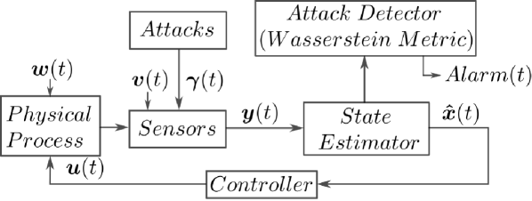
A remotely-observed, cyber-physical system subject to sensor-measurement attacks, as in Fig. 1, is described as a discrete-time, stochastic, linear, and time-invariant system
| (1) | ||||
where , and denote the system state, input and output at time , respectively. The state matrix , input matrix and output matrix are assumed to be known in advance. In particular, we assume that the pair is stabilizable, and is detectable. The process noise and output noise are independent zero-mean random vectors. We assume that each and are independent and identically distributed (i.i.d.) over time. We denote their (unknown, not-necessarily equal) distributions by and , respectively. In addition, we assume that and are light-tailed111 For a random vector such that , we say is -light-tailed, , if for some and . All examples listed have a moment generating function, so their exponential moment can be constructed for at least ., excluding scenarios of systems operating under extreme events, or subject to large delays. In fact, Gaussian, Sub-Gaussian, Exponential distributions, and any distribution with a compact support set are admissible. This class of distributions is sufficient to characterize the uncertainty or noise of many practical problems.
An additive sensor-measurement attack is implemented via in (1), on which we assume the following {assumption}[Attack model] It holds that 1) whenever there is no attack; 2) the attacker can modulate any component of at any time; 3) the attacker has unlimited computational resources and access to system information, e.g., , , , , and to decide on , .
II-A Normal System Operation
In what follows, we introduce the state observer that enables prediction in the absence of attacks (when ). Since the distribution of system noise is unknown, we identify a benchmark distribution that can be used to characterize this unknown distribution with high confidence.
To predict (estimate) the system behavior, we leverage the system information and employ a Kalman filter
where is the state estimate and is the steady-state Kalman gain matrix. As the pair is detectable, the gain can be selected in such a way that the eigenvalues of are inside the unit circle. This ensures asymptotic tracking of the state in expectation; that is, the expectation of the estimation error satisfies
The further selection of eigenvalues of and the structure of usually depends on additional control objectives such as noise attenuation requirements. In this paper, we additionally consider the estimated state feedback
where is so that the following augmented system is stable222System (2) is input-to-state stable in probability (ISSp) relative to any compact set which contains the origin, if we select such that eigenvalues of the matrix are inside the unit circle, see e.g. [15].
| (2) |
where , ,
Remark II.1 (Selection of and ).
In general, the selection of the matrices and for the system (1) is a nontrivial task, especially when certain performance criteria are to be satified, such as fast system response, energy conservation, or noise minimization. However, there are a few scenarios in which the Separation Principle can be invoked for a tractable design of and . For example, 1) when there is no system noise, matrices and can be designed separately, such that each and have all eigenvalues contained inside the unit circle, respectively. 2) when noise are Gaussian, the gain matrices and can be designed to minimize the steady-state covariance matrix and control effort, via a separated design of a Kalman filter (as an observer) and a linear-quadratic regulator (as a controller). The resulting design is referred to as a Linear-Quadratic-Gaussian (LQG) control [16].
Consider the system initially operates normally with the proper selection of and , and assume that the augmented system (2) is in steady state, i.e., . In order to design an attack detector later, we need a characterization of the distribution of the residue , which measures the difference between what we measure and what we expect to receive, as follows
When there is no attack, it can be verified that the random vector is zero-mean, and light-tailed333This can be checked from the definition in the footnote 1, and the fact that is a linear combination of zero-mean -light-tailed distributions., and we denote its unknown distribution by . We assume that a finite but large number of i.i.d. samples of are accessible, and acquired by collecting for a sufficiently large time. We call these i.i.d. samples a benchmark data set, , and construct the resulting empirical distribution by
where the operator is the mass function and the subscript indicates that is the benchmark to approximate the unknown . We can claim that, the benchmark provides a good sense of the effect of the noise on the system (2) via the following measure concentration result
Theorem II.1 (Measure Concentration [17, Application of Theorem 2]).
If is a -light-tailed distribution for some , then for a given , the following holds
where denotes the Probability, denotes the -Wasserstein metric444 Let denote the space of all -light-tailed probability distributions supported on . Then for any two distributions , , the -Wasserstein metric [18] is defined by where is in a set of all the probability distributions on with marginals and . The cost is a norm on . in the probability space, and the parameter is selected as
| (3) |
for some constant555The parameter is determined as in the definition of and the constants , depend on , , and (via , , ). When information on is absent, the parameters , and can be determined in a data-driven fashion using sufficiently many samples of . See [17] for details. , , , and is such that
or
where is the dimension of .
Theorem II.1 provides a probabilistic bound on the -Wasserstein distance between and , with a confidence at least . The result indicates how to tune the parameter and the number of benchmark samples that are needed to find a sufficiently good approximation of , by means of . In this way, given a fixed , we can increase our confidence () on whether and are within distance , by increasing the number of samples. We assume that has been determined in advance, selecting a very large (unique) to ensure various very small bounds associated with various . Later, we discuss how the parameter can be interpreted as a false alarm rate in the proposed attack detector. The resulting , with a tunnable false alarm rate (depending on ), will allow us to design a detection procedure which is robust to the system noise.
III Threshold-based robust detection of attacks, and stealthiness
This section presents our online detection procedure, and a threshold-based detector with high-confidence performance guarantees. Then, we propose a tractable computation of the detection measure used for online detection. We finish the section by introducing a class of stealthy attacks.
Online Detection Procedure (ODP): At each time , we construct a -step detector distribution
where is the residue data collected independently at time , for . Then with a given and a threshold , we consider the detection measure
| (4) |
and the attack detector
| (5) |
with the sequence of alarms generated online based on the previous threshold.
The distribution uses a small number of samples to ensure the online computational tractability of , so is highly dependent on instantaneous samples. Thus, may significantly deviate from the true , and from . Therefore, even if there is no attack, the attack detector is expected to generate false alarms due to the system noise as well as an improper selection of the threshold . In the following, we discuss how to select an that is robust to the system noise and which results in a desired false alarm rate. Note that the value should be small to be able to distinguish attacks from noise, as discussed later.
Lemma III.1 (Selection of for Robust Detectors).
Given parameters , , , , and a desired false alarm rate at time , if we select the threshold as
where is chosen as in (3) and is selected following the -formula (3), but with and in place of and , respectively. Then, the detection measure (4) satisfies
for any zero-mean -light-tailed underlying distribution .
Due to space limit, please see ArXiv version [19] for proofs.
Proof.
The proof leverages the triangular inequality
the measure concentration result for each term, and that samples of and are collected independently.
Lemma III.1 ensures that the false alarm rate is no higher than when there is no attack, i.e.,
Note that the rate can be selected by properly choosing the threshold . Intuitively, if we fix all the other parameters, then the smaller the rate , the larger the threshold . Also, large values of , , contribute to small .
Remark III.1 (Comparison with -detector).
Consider an alternative detection measure
where is the constant covariance matrix of the residue under normal system operation. In particular, if is Gaussian, the detection measure is -distributed and referred to as detection measure with degree of freedom. The detector threshold is selected via look-up tables of distribution, given the desired false alarm rate . To compare with , we leverage the assumption that is Gaussian with the given covariance . This gives explicitly the expression of the following
By selecting , we have
Note that, the measure-of-concentration result in Theorem II.1 is sharp when is Gaussian, which in fact results in the threshold as tight as that derived for -detector.
Computation of detection measure: To achieve a tractable computation of the detection measure , we leverage the definition of the Wasserstein distance (see footnote 4) and the fact that both and are discrete. The solution is given as a linear program.
The Wasserstein distance , originally solving the Kantorovich optimal transport problem [18], can be interpreted as the minimal work needed to move a mass of points described via a probability distribution , on the space , to a mass of points described by the probability distribution on the same space, with some transportation cost . The minimization that defines is taken over the space of all the joint distributions on whose marginals are and , respectively.
Assuming that both and are discrete, we can equivalently characterize the joint distribution as a discrete mass optimal transportation plan [18]. To do this, let us consider two sets and . Then, can be parameterized (by ) as follows
| (6) | ||||
| (7) |
Note that this characterizes all the joint distributions with marginals and , where is the allocation of the mass from to . Then, the proposed detection measure in (4) reduces to the following
| (P) | ||||
which is a linear program over a compact polyhedral set. Therefore, the solution exists and (P) can be solved to global optimal in polynomial time by e.g., a CPLEX solver.
III-A Detection and Stealthiness of Attacks
Following from the previous discussion, we now introduce a False Alarm Quantification Problem, then specialize it to the Attack Detection Problem considered in this paper. In particular, we analyze the sensitivity of the proposed attack detector method for the cyber-physical system under attacks.
Problem 1. (False Alarm Quantification Problem): Given the augmented system (2), the online detection procedure in Section III, and the attacker type described in Assumption 1, compute the false alarm rate
Problem 1, on the computation of the false alarm probability, requires prior information of the attack probability . In this work, we are interested in stealthy attacks, i.e., attacks that cannot be effectively detected by (5). We are led to the following problem.
Problem 2. (Attack Detection Problem): Given the setting of Problem 1, provide conditions that characterize stealthy attacks, i.e., attacks that contribute to , and quantify their impact on the system.
To remain undetected, the attacker must select such that is limited to within the threshold . To quantify the effects of these attacks, let us consider an attacker sequence backward in time with length . At time , denote the arbitrary injected attacker sequence by , (if , assume ). This sequence, together with (2), results in a detection sequence that can be used to construct detector distribution and detection measure . For simplicity and w.l.o.g., let us assume that is in the following form
| (8) |
where is any vector selected by the attacker.666 Note that, when there is no attack at , we have , resulting in . Similar techniques appearred in, e.g., [9, 20]. We characterize the scenarios that can occur, providing a first, partial answer to Problem 2. Then, we will come back to characterizing the impact of stealthy attacks in Section IV.
Definition III.1 (Attack Detection Characterization).
Assume (2) is subject to attack, i.e., for some .
-
•
If , , then the attack is stealthy with probability one, i.e., .
-
•
If , , then the attack is -step stealthy.
-
•
If , , then the attack is active with probability one, i.e., .
Lemma III.2 (Stealthy Attacks Leveraging System Noise).
Proof.
Assume (2) is under attack. Then, we prove the statement leveraging the measure concentration
which holds as is constructed using samples of , and the triangular inequality
resulting in with probability at least .
Note that , which allows the attacker to select with . However, the probability of being stealthy can be indefinitely low, with the range .
IV Stealthy Attack Analysis
In this section, we address the second question in Problem 2 via reachable-set analysis. In particular, we achieve an outer-approximation of the finite-step probabilistic reachable set, quantifying the effect of the stealthy attacks and the system noise in probability.
Consider an attack sequence as in (8), where is any vector such that the attack remains stealthy. That is, results in the detected distribution , which is close to as prescribed by . This results in the following representation of the system (2)
| (9) |
We provide in the following remark an intuition of how restrictive the stealthy attacker’s action has to be.
Remark IV.1 (Constant attacks).
Consider a constant offset attack for some , . Then by (P),
To ensure stealth, we require , this then limits the selection of in a ball centered at with radius . Note that the radius can be arbitrarily small by choosing the benchmark size large.
To quantify the reachable set of the system under attacks, prior information on the process noise is needed. To characterize , let us assume that, similarly to the benchmark , we are able to construct a noise benchmark distribution, denoted by . As before,
for some . Given certain time, we are interested in where, with high probability, the state of the system can evolve from some . To do this, we consider the -step probabilistic reachable set defined as follows
then the true system state at time , , satisfies
where accounts for the independent restriction of the unknown distributions to be “close” to its benchmark.
The exact computation of is intractable due to the unbounded support of the unknown distributions and , even if they are close to their benchmark. To ensure a tractable approximation, we follow a two-step procedure. First, we equivalently characterize the constraints on by its probabilistic support set. Then, we outer-approximate the probabilistic support by ellipsoids, and then the reachable set by an ellipsoidal bound.
Step 1: (Probabilistic Support of ) We achieve this by leveraging 1) the Monge formulation [18] of optimal transport, 2) the fact that is discrete, and 3) results from coverage control [21, 22]. W.l.o.g., let us assume is non-atomic (or continuous) and, consider the distribution and supported on . Let us denote by the transport map that assigns mass over from to . The Monge formulation of optimal transport aims to find an optimal transport map that minimizes the transportation cost as follows
It is known that if an optimal transport map exists, then the optimal transportation plan exists and the two problems and coincide777This is because the Kantorovich transport problem is the tightest relaxation of the Monge transport problem. See e.g., [18] for details.. In our setting, for strongly convex , and by the fact that is absolutely continuous, a unique optimal transport map can indeed be guaranteed888The Monge formulation is not always well-posed, i.e., there exists optimal transportation plans while transport map does not exist [18]., and therefore, .
Let us now consider any transport map of , and define a partition of the support of by
where are samples in , which generate . Then, we equivalently rewrite the value of the objective function defined in , as
| (10) |
where the constraints come from the fact that a transport map should lead to consistent calculation of set volumes under and , respectively. This results in the following equivalent problem to as
| (P1) | ||||
Given the distribution , Problem (P1) reduces to a load-balancing problem as in [22]. Let us define the Generalized Voronoi Partition (GVP) of associated to the sample set and weight , for all , as
It has been established that the optimal Partition of (P1) is the GVP [22, Proposition V.1]. Further, the standard Voronoi partition, i.e., the GVP with equal weights , results in a lower boundof (P1), when constraints (10) are removed [21], and therefore that of . We denote this lower bound as , and use this to quantify a probabilistic support of . Let us consider the support set
where . Then we have the following lemma.
Lemma IV.1 (Probabilistic Support).
Let and let be a distribution such that . Then, for any given , at least portion of the mass of is supported on , i.e., .
Proof.
Suppose otherwise, i.e., . Then,
In this way, the support contains at least of the mass of all the distributions such that . Equivalently, we have
where the random variable has a distribution such that . We characterize similarly.
Note that in practice, one can choose ball radius factor large in order to generate support which contains higher portion of the mass of unknown . However, it comes at a cost on the approximation of the reachable set.
Step 2: (Outer-approximation of ) Making use of the probabilistic support, we can now obtain a finite-dimensional characterization of the probabilistic reachable set, as follows
and the true system state at time , , satisfies Many works focus on the tractable evolution of geometric shapes; e.g. [9, 13]. Here, we follow [13] and propose outer ellipsoidal bounds for . Let be the positive-definite shape matrix such that . Similarly, we denote and for that of . We now state the following lemma, that applies [13, Proposition 1] for our case.
Lemma IV.2 (Outer bounds of ).
A tight reachable set bound can be now derived by solving
| (P2) | ||||
which is a convex semidefinite program, solvable via e.g., SeDuMi [23]. Note that the probabilistic reachable set is
which again can be approximated via solving (P2) for999The set is in fact contained in the projection of onto the state subspace, i.e., with . See, e.g., [13] for details.
V Simulations
In this section, we demonstrate the performance of the proposed attack detector, illustrating its distributional robustness w.r.t. the system noise. Then, we consider stealthy attacks as in (8) and analyze their impact by quantifying the probabilistic reachable set and outer-approximation bound.
Consider the stochastic system (2), given as
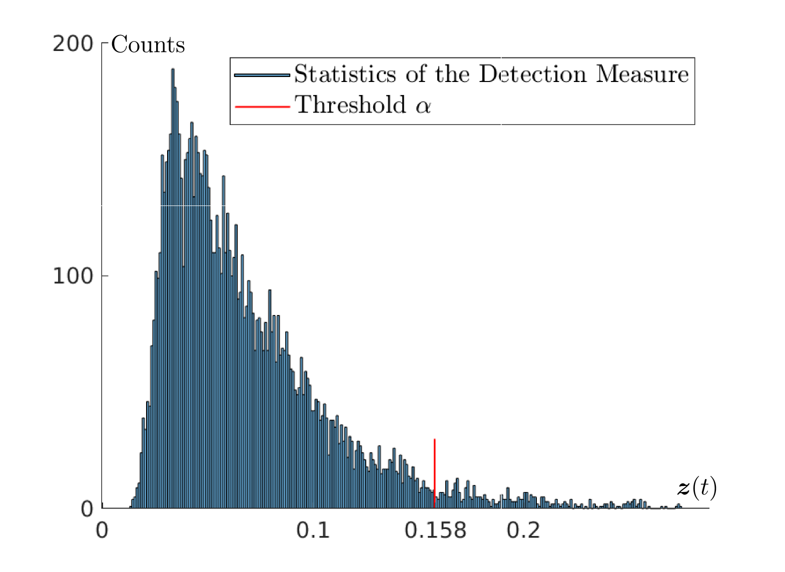
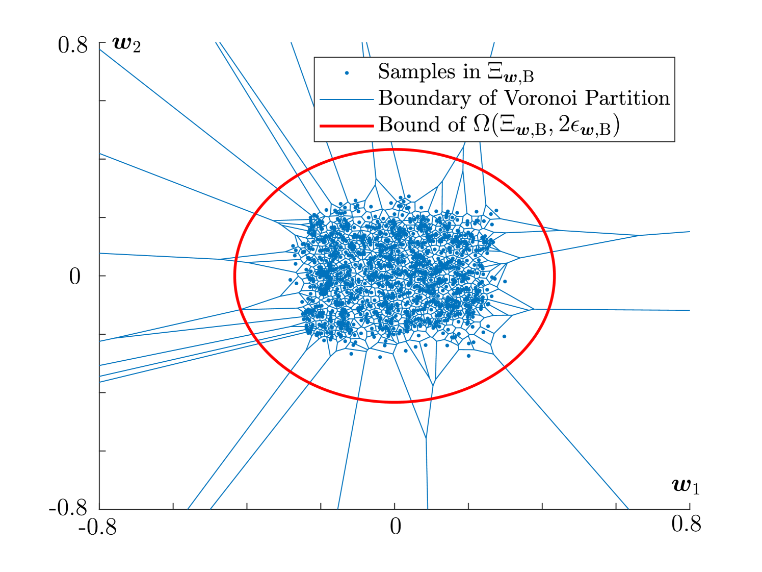
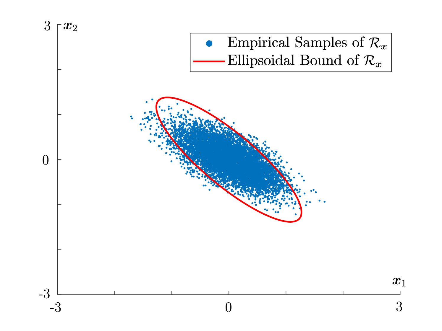
where and represent the normal and uniform distributions, respectively. We consider benchmark samples for and real-time samples for . We select the parameter , and false alarm rate . We select the prior information of the system noise via parameters , and . Using the measure-of-concentration results, we determine the detector threshold to be . In the normal system operation (no attack), we run the online detection procedure for time steps and draw the distribution of the computed detection measure as in Fig. 4. We verify that the false alarm rate is , within the required rate . When the system is subject to stealthy attacks, we assume and visualize the Voronoi partition (convex sets with blue boundaries) of the probabilistic support and its estimated ellipsoidal bound (red line) as in Fig. 4. Further, we demonstrate the impact of the stealthy attacks (8), as in Fig. 4. We used empirical points of as its estimate and provided an ellipsoidal bound of computed by solution of (P2). It can be seen that the proposed probabilistic reachable set effectively captures the reachable set in probability. Due to the space limits, we omit the comparison of our approach to the existing ones, such as the classical detector in [9] and the CUMSUM procedure [8]. However, the difference should be clear: our proposed approach is robust w.r.t. noise distributions while others leverage the moment information up to the second order, which only capture sufficient information about certain noise distributions, e.g., Gaussian.
VI Conclusions
A novel detection measure was proposed to enable distributionally robust detection of attacks w.r.t. unknown, and light-tailed system noise. The proposed detection measure restricts the behavior of the stealthy attacks, whose impact was quantified via reachable-set analysis.
References
- [1] A. Cardenas, S. Amin, B. Sinopoli, A. Giani, A. Perrig, and S. Sastry, “Challenges for securing cyber physical systems,” in Workshop on Future Directions of Cyber-Physical Systems, vol. 5, no. 1, 2009.
- [2] F. Pasqualetti, F. Dorfler, and F. Bullo, “Attack detection and identification in cyber-physical systems,” IEEE Transactions on Automatic Control, vol. 58, no. 11, p. 2715–2729, 2013.
- [3] S. Amin, A. Cardenas, and S. S. Sastry, “Safe and secure networked control systems under denial-of-service attacks,” in Hybrid systems: Computation and Control, 2009, p. 31–45.
- [4] F. Miao, Q. Zhu, M. Pajic, and G. J. Pappas, “Coding schemes for securing cyber-physical systems against stealthy data injection attacks,” IEEE Transactions on Control of Network Systems, vol. 4, no. 1, pp. 106–117, 2016.
- [5] C. Bai, F. Pasqualetti, and V. Gupta, “Data-injection attacks in stochastic control systems: Detectability and performance tradeoffs,” Automatica, vol. 82, pp. 251–260, 2017.
- [6] Y. Mo and B. Sinopoli, “Secure control against replay attacks,” in Allerton Conf. on Communications, Control and Computing, Illinois, USA, September 2009, pp. 911–918.
- [7] M. Zhu and S. Martínez, “On the performance analysis of resilient networked control systems under replay attacks,” IEEE Transactions on Automatic Control, vol. 59, no. 3, pp. 804–808, 2014.
- [8] J. Milošević, D. Umsonst, H. Sandberg, and K. Johansson, “Quantifying the impact of cyber-attack strategies for control systems equipped with an anomaly detector,” in European Control Conference, 2018, pp. 331–337.
- [9] Y. Mo and B. Sinopoli, “On the performance degradation of cyber-physical systems under stealthy integrity attacks,” IEEE Transactions on Automatic Control, vol. 61, no. 9, pp. 2618–2624, 2015.
- [10] S. Mishra, Y. Shoukry, N. Karamchandani, S. Diggavi, and P. Tabuada, “Secure state estimation against sensor attacks in the presence of noise,” IEEE Transactions on Control of Network Systems, vol. 4, no. 1, pp. 49–59, 2016.
- [11] C. Murguia, N. V. de Wouw, and J. Ruths, “Reachable sets of hidden CPS sensor attacks: Analysis and synthesis tools,” IFAC World Congress, vol. 50, no. 1, pp. 2088–2094, 2017.
- [12] C. Bai, F. Pasqualetti, and V. Gupta, “Security in stochastic control systems: Fundamental limitations and performance bounds,” in American Control Conference, 2015, pp. 195–200.
- [13] C. Murguia, I. Shames, J. Ruths, and D. Nesic, “Security metrics of networked control systems under sensor attacks,” arXiv preprint arXiv:1809.01808, 2018.
- [14] V. Renganathan, N. Hashemi, J. Ruths, and T. Summers, “Distributionally robust tuning of anomaly detectors in Cyber-Physical systems with stealthy attacks,” arXiv preprint arXiv:1909.12506, 2019.
- [15] A. R. Teel, J. P. Hespanha, and A. Subbaraman, “Equivalent characterizations of input-to-state stability for stochastic discrete-time systems,” IEEE Transactions on Automatic Control, vol. 59, no. 2, p. 516–522, 2014.
- [16] M. Athans, “The role and use of the stochastic linear-quadratic-Gaussian problem in control system design,” IEEE Transactions on Automatic Control, vol. 16, no. 6, pp. 529–552, 1971.
- [17] N. Fournier and A. Guillin, “On the rate of convergence in Wasserstein distance of the empirical measure,” Probability Theory and Related Fields, vol. 162, no. 3-4, p. 707–738, 2015.
- [18] F. Santambrogio, Optimal transport for applied mathematicians. Springer, 2015.
- [19] D. Li and S. Martínez, “High-confidence attack detection via Wasserstein-metric computations,” preprint arXiv:2003.07880, 2020.
- [20] C. Murguia and J. Ruths, “Cusum and chi-squared attack detection of compromised sensors,” in IEEE Conf. on Control Applications, 2016, pp. 474–480.
- [21] F. Bullo, J. Cortés, and S. Martínez, Distributed Control of Robotic Networks, ser. Applied Mathematics Series. Princeton University Press, 2009.
- [22] J. Cortés, “Coverage optimization and spatial load balancing by robotic sensor networks,” IEEE Transactions on Automatic Control, vol. 55, no. 3, pp. 749–754, 2010.
- [23] J. Sturm, “Using Sedumi 1.02, a MATLAB toolbox for optimization over symmetric cones,” Optimization Methods and Software, vol. 11, no. 1-4, pp. 625–653, 1999.