This paper was converted on www.awesomepapers.org from LaTeX by an anonymous user.
Want to know more? Visit the Converter page.

High-Dimensional Differentially-Private EM Algorithm: Methods and Near-Optimal Statistical Guarantees

Zhe Zhang and Linjun Zhang
Department of Statistics, Rutgers University
Abstract

In this paper, we develop a general framework to design differentially private expectation-maximization (EM) algorithms in high-dimensional latent variable models, based on the noisy iterative hard-thresholding. We derive the statistical guarantees of the proposed framework and apply it to three specific models: Gaussian mixture, mixture of regression, and regression with missing covariates. In each model, we establish the near-optimal rate of convergence with differential privacy constraints, and show the proposed algorithm is minimax rate optimal up to logarithm factors. The technical tools developed for the high-dimensional setting are then extended to the classic low-dimensional latent variable models, and we propose a near rate-optimal EM algorithm with differential privacy guarantees in this setting. Simulation studies and real data analysis are conducted to support our results.


Keywords: Differential privacy; High-dimensional data; EM algorithm; Optimal rate of convergence.

1 Introduction

In the era of big data, there is an unprecedented number of large data sets becoming available for researchers/industries to retrieve important information. In the meantime, these large data sets often include some sensitive personal information, urgently generating demands for privacy-preserving algorithms that can protect the individual information during the data analysis. One widely adopted criterion for privacy-preserving algorithms is differential privacy (DP) (Dwork et al., 2006b, a). This notion has been widely developed and used nowadays in Microsoft (Erlingsson et al., 2014), Google (Ding et al., 2017), Facebook (Kifer et al., 2020) and the U.S. Census Bureau (Abowd, 2016) to help protect individual privacy including user habits, browsing history, social connections, and health records. The basic idea behind differential privacy is that the information of a single individual in the training data should appear as hidden so that given the outcome, it is almost impossible to distinguish if a certain individual is in the dataset.

The attractiveness of differential privacy could possibly be attributed to the ease of building privacy-preserving algorithms. Many traditional algorithms and statistical methods have been extended to their private counterparts, including top-kk selection (Bafna and Ullman, 2017; Steinke and Ullman, 2017), multiple testing (Dwork et al., 2018), decision trees (Jagannathan et al., 2009), and random forests (Rana et al., 2015). However, many existing works only focus on designing privacy-preserving algorithms while lacking the sharp analysis of accuracy in terms of minimax optimality. At the high-level, these privatized algorithms are designed by injecting random noise into the traditional algorithms. Such noise-injection procedures typically sacrifice statistical accuracy, and therefore, it is essential to understand what is the best accuracy an algorithm would output while maintaining a certain level of differential privacy requirement. This motivates us to study the trade-off between the privacy and the statistical accuracy.

This paper is devoted to studying this trade-off in latent variable models by proposing a DP version of the expectation-maximization (EM) algorithm. The EM algorithm is a commonly used approach when dealing with latent variables and missing values Ranjan et al. (2016); Quost and Denoeux (2016); Kadir et al. (2014); Ding and Song (2016). The statistical properties, such as the local convergence and minimax optimality of standard EM algorithm has been recently studied in Balakrishnan et al. (2017); Wang et al. (2015); Yi and Caramanis (2015); Cai et al. (2019a); Zhao et al. (2020), while the development of DP EM algorithm, especially the theories of the optimal trade-off between privacy and accuracy, is still largely unexplored. In this paper, we propose novel DP EM algorithms in both the classic low-dimensional setting and the contemporary high-dimensional setting, where the parameter we are interested in is sparse and its dimension is greatly larger than the sample size. We demonstrate the superiority of the proposed algorithm by applying it to specific statistical models. Under these specific statistical models, the convergence rates of the proposed algorithm are found to be minimax optimal with privacy constraints. The main contributions of this paper are summarized in the following.

  • We design a novel DP EM algorithm in the high-dimensional setting based on a noisy iterative hard-thresholding algorithm in the M-step. Such a step effectively enforces the sparsity of the attained estimator while maintaining differential privacy, and allows us to establish sharp rate of convergence of the algorithm. To the best of our knowledge, this algorithm is the first DP EM algorithm in high-dimensions with statistical guarantees.

  • We then apply the proposed DP EM algorithm to three common models in the high-dimensional setting: Gaussian mixture model, mixture of regression model, and regression with missing covariates. Under mild regularity conditions, we show that our algorithm obtains the minimax optimal rate of convergence with privacy constraints.

  • In the classical low-dimensional setting, a DP EM algorithm based on the Gaussian mechanism is designed. The technical tools developed for the high-dimensional setting are then used to establish the optimality in this general low-dimensional setting. We show that both theoretically and numerically, the proposed algorithm outperforms several existing private EM algorithms in this classical setting.

Related Work. The expectation-maximization (EM) algorithm, proposed in (Dempster et al., 1977), is a common approach in handling latent variable models. There has been a long history on the study of the EM algorithm (Wu, 1983; McLachlan and Krishnan, 2007). Recently, a seminal work (Balakrishnan et al., 2017) obtains a general framework to study the statistical guarantees of EM algorithms in the classic low-dimensional setting. In subsequent works, the convergence rates of EM algorithm under various hidden variable models are studied, including the Gaussian mixture (Xu et al., 2016; Daskalakis et al., 2017; Yan et al., 2017; Kwon and Caramanis, 2020) and mixture of linear regression (Yi et al., 2014; Kwon et al., 2019, 2020). Another important direction is to design variants of EM algorithms in the high-dimensional regime. Such a goal is fulfilled through regularization (Cai et al., 2019a; Yi and Caramanis, 2015; Zhang et al., 2020) and truncation (Wang et al., 2015) in the M-step. Due to the increasing attention on data privacy nowadays, the design of private EM algorithms is in great demand but still largely lacking.

The differential privacy is arguably the most popular notion of privacy nowadays. After its invention, the basic properties has been studied in (Dwork et al., 2010; Dwork and Roth, 2014; Dwork et al., 2017; Dwork and Feldman, 2018; Mirshani et al., 2019). The trade-off between statistical accuracy and privacy is one of the fundamental topics in differential privacy. In the low-dimensional setting, there are various works focusing on this trade-off, including mean estimation (Dwork et al., 2015; Steinke and Ullman, 2016; Bun et al., 2018; Kamath et al., 2019; Cai et al., 2019b; Kamath et al., 2020b), confidence intervals of Gaussian mean (Karwa and Vadhan, 2017) and binomial mean (Awan and Slavković, 2020), linear regression (Wang, 2018; Cai et al., 2019b), generalized linear models Song et al. (2020); Cai et al. (2020); Song et al. (2021), principal component analysis (Dwork et al., 2014; Chaudhuri et al., 2013), convex empirical risk minimization (Bassily et al., 2014), and robust M-estimators (Avella-Medina, 2020; Avella-Medina et al., 2021).

However, in the high-dimensional setting where the dimension is much larger than the sample size, the trade-off between statistical accuracy and privacy is less studied. Most of the existing works focus on relatively standard statistical problems such as the sparse mean estimation and regression. For example, (Steinke and Ullman, 2017) studies the optimal bounds for private top-kk selection problems. (Cai et al., 2019b) studies near-optimal algorithms for the sparse mean estimation. For the high-dimensional sparse linear regression, (Talwar et al., 2015) obtains a DP LASSO algorithm which is near-optimal in terms of the excess risk; (Cai et al., 2019b) proposes another DP LASSO algorithm with the optimal rate of convergence in estimation. In (Cai et al., 2020), a near-minimax optimal DP algorithm for high-dimensional generalized linear models is introduced.

In the literature of differential privacy, most of the existing works for latent variable models focus on the low-dimensional cases, while the study in the high-dimensional regime is largely lacking. In the classical low-dimensional setting, (Park et al., 2017) introduces a DP EM algorithm, but offers no statistical guarantees/accuracy analysis. (Nissim et al., 2007) provides a result for the low-dimensional Gaussian mixture model based on the sample-aggregate framework and reaches a O(d3/nlog(1/δ)/ϵ)O(\sqrt{d^{3}/{n}}\cdot{\log(1/\delta)}/{\epsilon}) convergence rate in estimation for the mixture of spherical Gaussian distributions. (Kamath et al., 2020a) considers a more general Gaussian mixture models and studies the total variation distance. (Wang et al., 2020) studies the DP EM algorithm in the classical low-dimensional setting and obtains the estimation error of order O(d2/nlog(1/δ)/ϵ)O(\sqrt{d^{2}/{n}}\cdot{\log(1/\delta)}/{\epsilon}). In the current paper, we are going to show this rate can be significantly improved to O(d/n+dlog(1/δ)/nϵ)O(\sqrt{d/n}+{d\cdot\sqrt{\log(1/\delta)}}/{n\epsilon}), obtained by our proposed algorithm in the classic low-dimensional setting.

Organization of this paper. This paper is organized as follows. In Section 2, we introduce the problem formulation as well as some preliminaries of the EM algorithm and differential privacy. In Section 3, we present the main results of this paper and establish the convergence rate of the proposed EM algorithm in high-dimensional settings. In Section 4, we apply the results obtained in Section 3 to three specific models: Gaussian mixture model, mixture of regression, and regression with missing covariates. We present the estimation error bounds for these three models respectively and show the optimality. In Section 5, we consider the DP EM algorithm in the classic low-dimensional setting. In Section 6, simulation studies of the proposed algorithm are conducted to support our theory. Section 7 summarizes the paper and discusses some possible future work. In Appendix A, we provided some supplement materials. We prove the main results in Appendix B, and the proofs of other results and technical lemmas are in the Appendix C.

Notations. Throughout this paper, let 𝒗=(v1,v2,vd)d\bm{v}=(v_{1},v_{2},...v_{d})^{\top}\in\mathbb{R}^{d} be a vector. 𝒮\mathcal{S} denotes the set of indices and 𝒗𝒮\bm{v}_{\mathcal{S}} indicates the restriction of vector 𝒗\bm{v} on the set 𝒮\mathcal{S}. Also, 𝒗q\|\bm{v}\|_{q} denotes the q\ell_{q} norm for 1q1\leq q\leq\infty and 𝒗0\|\bm{v}\|_{0} specifically denotes the number of non-zero coordinates of 𝒗\bm{v}, and we also call it the sparsity level of 𝒗\bm{v}. We denote \odot to be the Hadamard product. Generally, we use nn to denote the number of samples, dd to denote the dimension of a vector and ss to denote the sparsity level of a vector. We also define a truncation function ΠT:dd\Pi_{T}:\mathbb{R}^{d}\rightarrow\mathbb{R}^{d} be a function denotes the projection into the \ell_{\infty} ball of radius TT centered at the origin in d\mathbb{R}^{d}. Moreover, we use Q(;)\nabla Q(\cdot;\cdot) to denote the gradient of the function Q(;)Q(\cdot;\cdot). If there is no further specification, this gradient is taken with respect to the first argument. For two sequences {an}\{a_{n}\} and {bn}\{b_{n}\}, we write an=o(bn)a_{n}=o(b_{n}) if an/bn0a_{n}/b_{n}\rightarrow 0. We denote an=O(bn)a_{n}=O(b_{n}) if there exist a constant cc such that ancbna_{n}\leq cb_{n} and an=Ω(bn)a_{n}=\Omega(b_{n}) if there exist a constant cc^{\prime} such that ancbna_{n}\geq c^{\prime}b_{n}. We also denote anbna_{n}\asymp b_{n} if an=O(bn)a_{n}=O(b_{n}) and an=Ω(bn)a_{n}=\Omega(b_{n}). In this paper, c0,c1,m0,m1,C,C,K,K,c_{0},c_{1},m_{0},m_{1},C,C^{\prime},K,K^{\prime},... denote universal constants and their specific values may vary from place to place.

2 Problem Formulation

In this section, we present some preliminaries that are important for the discussions in the rest of the paper. We are going to introduce the EM algorithm in Section 2.1, and the formal definition and some critical properties of differential privacy in Section 2.2.

2.1 The EM algorithm

The EM algorithm is a widely used algorithm to compute the maximum likelihood estimator when there are latent or unobserved variables in the model. We first introduce the standard EM algorithm. Let 𝒀\bm{Y} and 𝒁\bm{Z} be random variables taking values in the sample spaces 𝒴\mathcal{Y} and 𝒵\mathcal{Z}. For each pair of data (𝒀,𝒁)(\bm{Y},\bm{Z}), we assume that only 𝒀\bm{Y} is observed, while 𝒁\bm{Z} remains unobserved. Suppose that the pair (𝒀,𝒁)(\bm{Y},\bm{Z}) has a joint density function f𝜷(𝒚,𝒛)f_{\bm{\beta}^{*}}(\bm{y},\bm{z}), where 𝜷\bm{\beta}^{*} is the true parameter that we would like to estimate. Let h𝜷(𝒚)h_{\bm{\beta}^{*}}(\bm{y}) be the marginal density function of the observed variable 𝒀\bm{Y}. Then, we can write h𝜷(𝒚)h_{\bm{\beta}^{*}}(\bm{y}) by integrating out 𝒛\bm{z}

h𝜷(𝒚)=𝒵f𝜷(𝒚,𝒛)𝑑𝒛.h_{\bm{\beta}^{*}}(\bm{y})=\int_{\mathcal{Z}}f_{\bm{\beta}^{*}}(\bm{y},\bm{z})d\bm{z}. (1)

The goal of the EM algorithm is to obtain an estimator of 𝜷\bm{\beta}^{*} through maximizing the likelihood function. Specifically, suppose we have nn i.i.d.i.i.d. observations of 𝒀\bm{Y}: 𝒚1,𝒚2,𝒚nh𝜷(𝒚)\bm{y}_{1},\bm{y}_{2},...\bm{y}_{n}\sim h_{{\bm{\beta}}^{*}}(\bm{y}), we aim to use EM algorithm to maximize the log-likelihood ln(𝜷)=i=1nlogh𝜷(𝒚i)l_{n}(\bm{\beta})=\sum_{i=1}^{n}\log h_{\bm{\beta}}(\bm{y}_{i}), and get an estimator of 𝜷{\bm{\beta}}^{*}. In many latent variable models, it is generally difficult to evaluate the log-likelihood ln(𝜷)l_{n}(\bm{\beta}) directly, but relatively easy to compute the log-likelihood for the joint distribution f𝜷(𝒚,𝒛)f_{\bm{\beta}}(\bm{y},\bm{z}). Such situations are in need of EM algorithms. Specifically, for a given parameter 𝜷{\bm{\beta}}, let k𝜷(𝒛|𝒚)k_{\bm{\beta}}(\bm{z}|\bm{y}) be the conditional distribution of 𝒁\bm{Z} given the observed variable 𝒀\bm{Y}, that is, k𝜷(𝒛|𝒚)=f𝜷(𝒚,𝒛)h𝜷(𝒚).k_{\bm{\beta}}(\bm{z}|\bm{y})=\frac{f_{\bm{\beta}}(\bm{y},\bm{z})}{h_{\bm{\beta}}(\bm{y})}.

The EM algorithm uses an iterative approach motivated by Jensen’s inequality. Suppose that in the tt-th iteration, we have obtained 𝜷t{\bm{\beta}}^{t} and would like to update it to 𝜷t+1{\bm{\beta}}^{t+1} with a larger log-likelihood. The log-likelihood evaluated at 𝜷t+1\bm{\beta}^{t+1} can always be lower bounded, as shown in the following expression.

1nln(𝜷t+1)\displaystyle\frac{1}{n}l_{n}(\bm{\beta}^{t+1}) =1ni=1nlogh𝜷t+1(𝒚i)\displaystyle=\frac{1}{n}\sum_{i=1}^{n}\log h_{\bm{\beta}^{t+1}}(\bm{y}_{i}) (2)
1ni=1n𝒵k𝜷t(𝒛i|𝒚i)logf𝜷t+1(𝒚i,𝒛i)𝑑𝒛iQn(𝜷t+1;𝜷t)1ni=1n𝒵k𝜷t(𝒛i|𝒚i)logk𝜷t(𝒛i|𝒚i)𝑑𝒛i,\displaystyle\geq\underbrace{\frac{1}{n}\sum_{i=1}^{n}\int_{\mathcal{Z}}k_{{\bm{\beta}}^{t}}(\bm{z}_{i}|\bm{y}_{i})\log f_{\bm{\beta}^{t+1}}(\bm{y}_{i},\bm{z}_{i})d\bm{z}_{i}}_{Q_{n}({\bm{\beta}^{t+1}};{{\bm{\beta}}^{t}})}-\frac{1}{n}\sum_{i=1}^{n}\int_{\mathcal{Z}}k_{{\bm{\beta}}^{t}}(\bm{z}_{i}|\bm{y}_{i})\log k_{{\bm{\beta}}^{t}}(\bm{z}_{i}|\bm{y}_{i})d\bm{z}_{i},

with equality holds when 𝜷t+1=𝜷t{\bm{\beta}}^{t+1}={\bm{\beta}}^{t}. The basic idea of EM algorithm is to successively maximize the lower bound with respect to 𝜷t+1{\bm{\beta}}^{t+1} in (2). In the E-step, we evaluate the lower bound in (2) at the current parameter 𝜷t{\bm{\beta}}^{t}. Since the second term in (2) only depends on 𝜷t\bm{\beta}^{t}, which is fixed given the current 𝜷t{\bm{\beta}}^{t}, we only need to evaluate QnQ_{n} in the E-step. Then, in the M-Step, we calculate a new parameter 𝜷t+1{\bm{\beta}}^{t+1} which moves towards the direction that maximizes QnQ_{n}, so the lower bound in (2) becomes larger when we update 𝜷t{\bm{\beta}}^{t} to 𝜷t+1{\bm{\beta}}^{t+1}. We use the new parameter 𝜷t+1{\bm{\beta}}^{t+1} at the (t+1)(t+1)-th iteration and continue the E-step and M-step iteratively until convergence.

In the tt-th iteration, the M-step in the standard EM algorithm maximizes Qn(;𝜷t)Q_{n}(\cdot;\bm{\beta}^{t}) (Dempster et al., 1977), that is, 𝜷t+1=argmax𝜷Qn(𝜷;𝜷t)\bm{\beta}^{t+1}=\text{argmax}_{\bm{\beta}}Q_{n}(\bm{\beta};\bm{\beta}^{t}). However, sometimes it is computationally expensive to compute the maximizer directly. As an alternative, the gradient EM (Balakrishnan et al., 2017) was proposed by taking one-step update of the gradient ascent 𝜷t+1=𝜷t+ηQn(𝜷t;𝜷t)\bm{\beta}^{t+1}=\bm{\beta}^{t}+\eta\cdot\nabla Q_{n}(\bm{\beta}^{t};\bm{\beta}^{t}) in the M-step. When Qn(𝜷;𝜷)Q_{n}(\bm{\beta};\bm{\beta}^{\prime}) is strongly convex with respect to 𝜷{\bm{\beta}}, this gradient EM approach is shown to reach the same statistical guarantee as that of the standard EM approach (Balakrishnan et al., 2017). In the high-dimensional setting, when the data dimension is much larger than the sample size and the true parameter is sparse, people have come up with different variants of EM algorithms. For example, in the M-step, the maximization approach is generalized to the regularized maximization (Yi and Caramanis, 2015; Cai et al., 2019a; Zhang et al., 2020) and the gradient approach is generalized to the truncated gradient (Wang et al., 2015).

2.2 Some basic properties of differential privacy

In this section, we introduce the concepts and properties of differential privacy. These properties will play an important role in the design of the DP EM algorithm. First, the formal definition of differential privacy is given below.

Definition 2.1 (Differential Privacy (Dwork et al., 2006b)).

Let 𝒳\mathcal{X} be the sample space for an individual data, a randomized algorithm M:𝒳nM:\mathcal{X}^{n}\rightarrow\mathbb{R} is (ϵ,δ)(\epsilon,\delta)-DP if and only if for every pair of adjacent data sets 𝐗,𝐗𝒳n\bm{X},\bm{X}^{\prime}\in\mathcal{X}^{n} and for any SS\subseteq\mathbb{R}, the inequality below holds:

(M(𝑿)S)eε(M(𝑿)S)+δ,\displaystyle\mathbb{P}\left(M(\bm{X})\in S\right)\leq e^{\varepsilon}\cdot\mathbb{P}\left(M(\bm{X}^{\prime})\in S\right)+\delta,

where we say that two data sets 𝐗={𝐱i}i=1n\bm{X}=\{\bm{x}_{i}\}_{i=1}^{n} and 𝐗={𝐱i}i=1n\bm{X}^{\prime}=\{{{\bm{x}}_{i}^{\prime}}\}_{i=1}^{n} are adjacent if and only if they differ by one individual datum.

According to the definition, the two parameters ϵ,δ\epsilon,\delta control the privacy level. With smaller ϵ\epsilon and δ\delta, the privacy constraint becomes more stringent. Intuitively speaking, this definition suggests that for a DP algorithm MM, an adversary cannot distinguish if the original dataset is 𝑿\bm{X} or 𝑿\bm{X}^{\prime} when 𝑿\bm{X} and 𝑿\bm{X}^{\prime} is adjacent, implying that the information of each individual is protected after releasing MM.

We then list several useful facts of designing DP algorithms. To create a DP algorithm, the arguably most common strategy is to add random noise to the output. Intuitively, the scale of the noise can not be too large, otherwise the accuracy of the output will be sacrificed. This scale is characterized by the sensitivity of the algorithm.

Definition 2.2.

For any algorithm f:𝒳ndf:\mathcal{X}^{n}\rightarrow{\mathbb{R}}^{d} and two adjacent data sets 𝐗\bm{X} and 𝐗\bm{X}^{\prime}, the p\ell_{p}-sensitivity of ff is defined as: Δp(f)=sup𝐗,𝐗𝒳n adjacentf(𝐗)f(𝐗)p.\Delta_{p}(f)=\sup_{\bm{X},\bm{X}^{\prime}\in\mathcal{X}^{n}\text{ adjacent}}\|f(\bm{X})-f(\bm{X}^{\prime})\|_{p}.

For algorithms with finite 1\ell_{1}-sensitivity or 2\ell_{2}-sensitivity, we can achieve differential privacy by adding Laplace noises or Gaussian noises respectively.

Proposition 2.3 (The Laplace Mechanism (Dwork et al., 2006b)).

Let f:𝒳ndf:\mathcal{X}^{n}\to\mathbb{R}^{d} be a deterministic algorithm with Δ1(f)<\Delta_{1}(f)<\infty. For 𝐰d\bm{w}\in\mathbb{R}^{d} with coordinates w1,w2,,wdw_{1},w_{2},\cdots,w_{d} be i.i.d samples drawn from Laplace(Δ1(f)/ϵ)(\Delta_{1}(f)/\epsilon), f(𝐗)+𝐰f(\bm{X})+\bm{w} is (ϵ,0)(\epsilon,0)-DP.

Proposition 2.4 (The Gaussian Mechanism (Dwork et al., 2006b)).

Let f:𝒳ndf:\mathcal{X}^{n}\to\mathbb{R}^{d} be a deterministic algorithm with Δ2(f)<\Delta_{2}(f)<\infty. For 𝐰=(w1,w2,,wd)\bm{w}=(w_{1},w_{2},\cdots,w_{d}) with coordinates i.i.d drawn from N(0,2(Δ2(f)/ϵ)2log(1.25/δ))N(0,2(\Delta_{2}(f)/\epsilon)^{2}\log(1.25/\delta)), f(𝐗)+𝐰f(\bm{X})+\bm{w} is (ϵ,δ)(\epsilon,\delta)-DP.

These two mechanisms are computationally efficient, and are typically used to build more complicated algorithms. In the following, we introduce the post-processing and composition properties of differential privacy, which enable us to design complicated DP algorithms by combining simpler ones.

Proposition 2.5 (Post-processing Property (Dwork et al., 2006b)).

Let MM be an (ϵ,δ)(\epsilon,\delta)-DP algorithm and gg be an arbitrary function which takes M(𝐗)M(\bm{X}) as input, then g(M(𝐗))g(M(\bm{X})) is also (ϵ,δ)(\epsilon,\delta)-DP.

Proposition 2.6 (Composition property (Dwork et al., 2006b)).

For i=1,2i=1,2, let MiM_{i} be (εi,δi)(\varepsilon_{i},\delta_{i})-DP algorithm, then (M1,M2)(M_{1},M_{2}) is (ϵ1+ϵ2,δ1+δ2)(\epsilon_{1}+\epsilon_{2},\delta_{1}+\delta_{2})-DP algorithm.

In the following section, we will see that the above two properties are particularly useful in the design of the DP EM algorithm.

3 High-dimensional EM Algorithm

In this section, we develop a novel DP EM algorithm for the (sparse) high-dimensional latent variable models. We are going to first introduce the detailed description of the proposed algorithm in Section 3.1, and then present its theoretical properties in Section 3.2. We will further apply our general method to three specific models in the next section.

3.1 Methodology

Suppose we have i.i.di.i.d data sampled from the latent variable model (1) and aim to use the EM algorithm to find the maximum likelihood estimator in a DP manner. Since the EM algorithm is an iterative approach where the tt-th iteration takes as input the 𝜷t1{\bm{\beta}}^{t-1} from the M-step in the last iteration, it suffices to make each 𝜷t{\bm{\beta}}^{t} differentially private to ensure the privacy guarantee of the final output.

Our algorithm relies on two key designs in the M-step. First, we use the gradient EM approach, and in the gradient update stage, we introduce a truncation step on the gradient to control the sensitivity of the gradient update, and thus we can appropriately determine the scale of noise we need to achieve differential privacy. Secondly, we propose to apply the noisy hard-thresholding algorithm (NoisyHT) (Dwork et al., 2018) to pursue sparsity and achieve privacy at the same time. The NoisyHT algorithm is defined as follows,

2
1:vector-valued function 𝒗=𝒗(𝑿)d\bm{v}=\bm{v}(\bm{X})\in\mathbb{R}^{d} with data 𝑿\bm{X}, sparsity ss, privacy parameters ε,δ\varepsilon,\delta, sensitivity λ\lambda.
2:Initialization: S=S=\emptyset.
3:For ii in 11 to ss:
4: Generate 𝒘id\bm{w}_{i}\in\mathbb{R}^{d} with wi1,wi2,,widi.i.d.Laplace(λ23slog(1/δ)ε)w_{i1},w_{i2},\cdots,w_{id}\stackrel{{\scriptstyle\text{i.i.d.}}}{{\sim}}\text{Laplace}\left(\lambda\cdot\frac{2\sqrt{3s\log(1/\delta)}}{\varepsilon}\right)
5: Append j=argmaxj[d]S(|vj|+wij)j^{*}=\text{argmax}_{j\in[d]\setminus S}(|v_{j}|+w_{ij}) to SS
6:End For
7: Generate 𝒘~\tilde{\bm{w}} with w~1,,w~di.i.d.Laplace(λ23slog(1/δ)ε)\tilde{w}_{1},\cdots,\tilde{w}_{d}\stackrel{{\scriptstyle\text{i.i.d.}}}{{\sim}}\text{Laplace}\left(\lambda\cdot\frac{2\sqrt{3s\log(1/\delta)}}{\varepsilon}\right)
18:PS(𝒗+𝒘~)P_{S}(\bm{v}+\tilde{\bm{w}})
Algorithm 1 Noisy Hard Thresholding (NoisyHT(𝒗,s,λ,ϵ,δ\bm{v},s,\lambda,\epsilon,\delta)) (Dwork et al., 2018)

In the last step, PS(𝒖)P_{S}(\bm{u}) denotes the operator that makes 𝒖Sc=0\bm{u}_{S^{c}}=0 while preserving 𝒖S\bm{u}_{S}. A great advantage of this algorithm is that when the vector 𝒗=v(𝑿)\bm{v}=v(\bm{X}) has bounded \ell_{\infty} sensitivity λ\lambda, the algorithm is guaranteed to be DP, as we can see in the lemma below.

Lemma 3.1 ((Dwork et al., 2018)).

If for every pair of adjacent data sets 𝐗,𝐗𝒳n\bm{X},\bm{X}^{\prime}\in\mathcal{X}^{n}. we have v(𝐗)v(𝐗)<λ||v(\bm{X})-v(\bm{X}^{\prime})||_{\infty}<\lambda, then the noisy hard-thresholding algorithm is (ϵ,δ)(\epsilon,\delta)-DP.

Another important property of the NoisyHT algorithm is its accuracy. Specifically, for the coordinates that are not chosen by the NoisyHT algorithm, the 2\ell_{2} norm of these coordinates is upper bounded by that of the coordinates with the same size but chosen by the NoisyHT algorithm up to some error term. The formal statement is summarized in the following with the proof given in Appendix C.1.

Lemma 3.2.

Let SS be the set chosen by the NoisyHT algorithm, 𝐯\bm{v} be the input vector and {𝐰i}i[s]\{\bm{w}_{i}\}_{i\in[s]} be defined as in the NoisyHT algorithm. For every set R1SR_{1}\subset S and R2ScR_{2}\subset S^{c} such that |R1|=|R2||R_{1}|=|R_{2}| and for every c>0c>0, we have:

𝒗R222(1+c)𝒗R122+4(1+1/c)i[s]𝒘i2.||\bm{v}_{R_{2}}||_{2}^{2}\leq(1+c)||\bm{v}_{R_{1}}||_{2}^{2}+4\cdot(1+1/c)\sum_{i\in[s]}||\bm{w}_{i}||_{\infty}^{2}.

After introducing the NoisyHT algorithm, we now proceed to the development of the DP EM algorithm. We update the estimator 𝜷^\hat{\bm{\beta}} based on the NoisyHT algorithm in each M-step after truncation. Such a modified M-step guarantees that the output 𝜷t{\bm{\beta}}^{t} is sparse and differentially private in each iteration. We also note here that we use the sample-splitting in the algorithm, which makes 𝜷t{\bm{\beta}}^{t} independent with the batch of samples in tt-th iteration and helps control the sensitivity of the gradient. The algorithm is summarized below:

3
1:Private parameters (ϵ,δ)(\epsilon,\delta), step size η\eta, truncation level TT, maximum number of iterations N0N_{0}, sparsity parameter s^\hat{s}.
2:Initialization: 𝜷0\bm{\beta}^{0} with 𝜷00s^||\bm{\beta}^{0}||_{0}\leq\hat{s}.
3:For t=0,1,2,N01t=0,1,2,...N_{0}-1:
4: Compute 𝜷t+0.5=𝜷t+ηfT(Qn/N0(𝜷t;𝜷t))\bm{\beta}^{t+0.5}=\bm{\beta}^{t}+\eta\cdot f_{T}(\nabla Q_{n/N_{0}}(\bm{\beta}^{t};\bm{\beta}^{t})).
5: Let 𝜷t+1=NoisyHT(𝜷t+0.5,s^,2ηN0T/n,ϵ,δ)\bm{\beta}^{t+1}=\text{NoisyHT}(\bm{\beta}^{t+0.5},\hat{s},2\eta\cdot N_{0}\cdot T/n,\epsilon,\delta).
16:End For
27:𝜷^=𝜷N0\hat{{\bm{\beta}}}={\bm{\beta}}^{N_{0}}
Algorithm 2 High-Dimensional DP EM algorithm

In the above algorithm, the truncation operator fT(Qn(𝜷;𝜷))f_{T}(\nabla Q_{n}(\bm{\beta};\bm{\beta})) with truncation level TT is defined as fT(Qn(𝜷;𝜷))=1ni=1nhT(qi(𝜷;𝜷))f_{T}(\nabla Q_{n}(\bm{\beta};\bm{\beta}))=\frac{1}{n}\sum_{i=1}^{n}h_{T}(\nabla q_{i}(\bm{\beta};\bm{\beta})), where qi(𝜷;𝜷)=𝒵k𝜷(𝒛i|𝒚i)logf𝜷(𝒚i,𝒛i)𝑑𝒛iq_{i}(\bm{\beta};\bm{\beta})=\int_{\mathcal{Z}}k_{{\bm{\beta}}}(\bm{z}_{i}|\bm{y}_{i})\log f_{\bm{\beta}}(\bm{y}_{i},\bm{z}_{i})d\bm{z}_{i}, and hTh_{T} denotes some generic truncation function with \ell_{\infty} norm upper bounded by TT. Later in the application to different specific models, we will specify the form of hTh_{T} for each model. The next lemma shows Algorithm 2 is (ϵ,δ)(\epsilon,\delta)-DP.

Lemma 3.3.

The output of high-dimensional DP EM algorithm (Algorithm 2) is (ϵ,δ)(\epsilon,\delta)-DP.

The proof of Lemma 3.3 is given in the Appendix C.2. In theory, we shall take the truncation level TT and number of iterations N0N_{0} to be the order of logn\sqrt{\log n} and logn\log n, respectively, as we will show in the next section. For the sparsity level s^\hat{s}, we should choose it to have the same order of the true sparsity level ss^{*}. While the true parameter ss^{*} is unknown in practice, s^\hat{s} could be chosen through cross-validation. Given the differential privacy guarantees, we are going to analyze the utility of this algorithm in the next section.

3.2 Theoretical gaurantees

In this section, we analyze the theoretical properties of the proposed high-dimensional DP EM algorithm. Before we lay out the main results, we first introduce four technical conditions. The first three conditions are standard in the literature of EM algorithms; for example, see (Balakrishnan et al., 2017; Wang et al., 2015; Zhu et al., 2017; Wang et al., 2020). The fourth condition is needed to control the sensitivity in the design of DP algorithms. We will verify these four conditions in the specific models in the next section.

Condition 3.4 (Lipschitz-Gradient(γ,)(\gamma,\mathcal{B})).

For the true parameter 𝛃\bm{\beta}^{*} and any 𝛃\bm{\beta}\in\mathcal{B}, where \mathcal{B} denotes a region in the parameter space. We have

Q(𝜷;𝜷)Q(𝜷;𝜷)2γ𝜷𝜷2.||\nabla Q(\bm{\beta};\bm{\beta}^{*})-\nabla Q(\bm{\beta};\bm{\beta})||_{2}\leq\gamma||\bm{\beta}-\bm{\beta}^{*}||_{2}.

This condition implies that if 𝜷\bm{\beta} is close to the true parameter 𝜷\bm{\beta}^{*}, then the gradients Q(𝜷;𝜷)\nabla Q(\bm{\beta};\bm{\beta}^{*}) and Q(𝜷;𝜷)\nabla Q(\bm{\beta};\bm{\beta}) should also be close, which implies gradient stability.

Condition 3.5 (Concavity-Smoothness (μ,ν,)(\mu,\nu,\mathcal{B})).

For any 𝛃1,𝛃2\bm{\beta}_{1},\bm{\beta}_{2}\in\mathcal{B}, Q(;𝛃)Q(\cdot;\bm{\beta}^{*}) is μ\mu-smooth such that

Q(𝜷1;𝜷)Q(𝜷2;𝜷)+𝜷1𝜷2,Q(𝜷2;𝜷)μ/2𝜷2𝜷122,Q(\bm{\beta}_{1};\bm{\beta}^{*})\geq Q(\bm{\beta}_{2};\bm{\beta}^{*})+\langle\bm{\beta}_{1}-\bm{\beta}_{2},\nabla Q(\bm{\beta}_{2};\bm{\beta}^{*})\rangle-\mu/2\cdot||\bm{\beta}_{2}-\bm{\beta}_{1}||_{2}^{2},

and ν\nu-strongly concave such that

Q(𝜷1;𝜷)Q(𝜷2;𝜷)+𝜷1𝜷2,Q(𝜷2;𝜷)ν/2𝜷2𝜷122.Q(\bm{\beta}_{1};\bm{\beta}^{*})\leq Q(\bm{\beta}_{2};\bm{\beta}^{*})+\langle\bm{\beta}_{1}-\bm{\beta}_{2},\nabla Q(\bm{\beta}_{2};\bm{\beta}^{*})\rangle-\nu/2\cdot||\bm{\beta}_{2}-\bm{\beta}_{1}||_{2}^{2}.

The Concavity-Smoothness condition indicates that when the second argument of Q(;)Q(\cdot;\cdot) is 𝜷\bm{\beta}^{*}, Q(;)Q(\cdot;\cdot) is a well-behaved convex function that it can be upper bounded and lower bounded by two quadratic functions. This condition ensures the geometric decay of the optimization error in the statistical analysis.

Condition 3.6 (Statistical-Error(α,τ,s,n,)(\alpha,\tau,s,n,\mathcal{B})).

For any fixed 𝛃\bm{\beta}\in\mathcal{B} and 𝛃0s||\bm{\beta}||_{0}\leq s, we have with probability at least 1τ1-\tau,

Q(𝜷;𝜷)Qn(𝜷;𝜷)α.||\nabla Q(\bm{\beta};\bm{\beta})-\nabla Q_{n}(\bm{\beta};\bm{\beta})||_{\infty}\leq\alpha.

In this condition, the statistical error is quantified by the \ell_{\infty} norm between the population quantity Q(𝜷;𝜷)\nabla Q(\bm{\beta};\bm{\beta}) and its sample version Qn(𝜷;𝜷)\nabla Q_{n}(\bm{\beta};\bm{\beta}). Such a bound is different from the 2\ell_{2} norm bound considered in the classic low-dimensional DP EM algorithms (Wang et al., 2020). In the high-dimensional setting, although for each index, the statistical error is small, the 2\ell_{2} norm can still be quite large. This fine-grained \ell_{\infty} bound enables us to iteratively quantify the statistical accuracy when using the NoisyHT in the M-step.

Condition 3.7 (Truncation-Error(ξ,ϕ,s,n,T,)(\xi,\phi,s,n,T,\mathcal{B})).

For any 𝛃\bm{\beta}\in\mathcal{B} and 𝛃0s\|\bm{\beta}\|_{0}\leq s, there exists a non-incresaing function ϕ\phi, such that for the truncation level TT, with probability 1ϕ(ξ)1-\phi(\xi),

Qn(𝜷;𝜷)fT(Qn(𝜷;𝜷))2ξ.||\nabla Q_{n}(\bm{\beta};\bm{\beta})-f_{T}(\nabla Q_{n}(\bm{\beta};\bm{\beta}))||_{2}\leq\xi.

The Truncation-Error condition quantifies the error caused by the truncation step in Algorithm 2. Intuitively, when TT is large, the truncation error ξ\xi can be very small, while leading to larger sensitivity and larger injected noise to ensure privacy. We need to carefully choose TT to strike a balance between the statistical accuracy and privacy cost. Below we show the main result of this section, with the detailed proof given in Section B.1.

Theorem 3.8.

Suppose the true parameter 𝛃\bm{\beta}^{*} is sparse with 𝛃0s\|\bm{\beta}^{*}\|_{0}\leq s^{*}. We define ={𝛃:𝛃𝛃2R}\mathcal{B}=\{\bm{\beta}:||\bm{\beta}-\bm{\beta}^{*}||_{2}\leq R\} with R=L𝛃2R=L\cdot\|\bm{\beta}^{*}\|_{2} for some L(0,1)L\in(0,1). We assume the Concavity-Smoothness(μ,ν,)(\mu,\nu,\mathcal{B}) holds and the initialization 𝛃0\bm{\beta}^{0} satisfies 𝛃0𝛃2R/2||\bm{\beta}^{0}-\bm{\beta}^{*}||_{2}\leq R/2. We further assume that the Lipschitz-Gradient(γ,)(\gamma,\mathcal{B}) holds and define κ=12νγν+μ(0,1)\kappa=1-2\cdot\frac{\nu-\gamma}{\nu+\mu}\in(0,1). In Algorithm 2, we let the step size η=2/(μ+ν)\eta=2/(\mu+\nu), the number of iterations N0lognN_{0}\asymp\log n, the sparsity level s^c0max(16(1/κ1)2,4(1+L)2(1L)2)s\hat{s}\geq c_{0}\cdot\max(\frac{16}{(1/\kappa-1)^{2}},\frac{4\cdot(1+L)^{2}}{(1-L)^{2}})\cdot s^{*} where c0c_{0} is a constant greater than 1 and s^=O(s)\hat{s}=O(s^{*}). We assume the condition Truncation-Error(ξ,ϕ,s^,n/N0,T,\xi,\phi,\hat{s},n/N_{0},T,\mathcal{B}) holds with TlognT\asymp\sqrt{\log n} and ϕ(ξ)N0=o(1)\phi(\xi)\cdot N_{0}=o(1). Moreover, we assume the condition Statistical-Error(α,τ/N0,s^,n/N0,)(\alpha,\tau/{N_{0}},\hat{s},n/{N_{0}},\mathcal{B}) holds and assume that α=o(1)\alpha=o(1) and there exists a constant c1>0c_{1}>0, and (s^+c1/1Ls)ηαmin((1κ)2R,(1L)22(1+L)β2)(\sqrt{\hat{s}}+c_{1}/\sqrt{1-L}\cdot\sqrt{s^{*}})\cdot\eta\cdot\alpha\leq\min((1-\sqrt{\kappa})^{2}\cdot R,\frac{(1-L)^{2}}{2\cdot(1+L)}\cdot\|\beta^{*}\|_{2}), also slogdn(logn)32=o(1)\frac{s^{*}\log d}{n}\cdot(\log n)^{\frac{3}{2}}=o(1). Then there exist constants K,m0,m1K,m_{0},m_{1}, it holds that

𝜷t𝜷2\displaystyle\|\bm{\beta}^{t}-\bm{\beta}^{*}\|_{2} κt/2𝜷0𝜷2+(s^+c1/1Ls)η1κα+Kslogdlog(1/δ)log3/2nnϵ\displaystyle\leq\kappa^{t/2}\cdot||{\bm{\beta}}^{0}-\bm{\beta}^{*}||_{2}+\frac{(\sqrt{\hat{s}}+c_{1}/\sqrt{1-L}\cdot\sqrt{s^{*}})\cdot\eta}{1-\sqrt{\kappa}}\cdot\alpha+K\cdot\frac{s^{*}\cdot\log d\cdot\sqrt{\log(1/\delta)}\log^{3/2}n}{n\epsilon}
+ηξ/(1κ),\displaystyle+\eta\cdot\xi/(1-\sqrt{\kappa}), (3)

with probability 1τN0ϕ(ξ)m0slognexp(m1logd)1-\tau-N_{0}\cdot\phi(\xi)-m_{0}\cdot s^{*}\cdot\log n\cdot\exp(-m_{1}\log d). Specifically, for the output in Algorithm 2, it holds that

𝜷N0𝜷2\displaystyle\|\bm{\beta}^{N_{0}}-\bm{\beta}^{*}\|_{2} (s^+c1/1Ls)η1κα+Kslogdlog(1/δ)log3/2nnϵ+ηξ/(1κ),\displaystyle\leq\frac{(\sqrt{\hat{s}}+c_{1}/\sqrt{1-L}\cdot\sqrt{s^{*}})\cdot\eta}{1-\sqrt{\kappa}}\cdot\alpha+K\cdot\frac{s^{*}\cdot\log d\cdot\sqrt{\log(1/\delta)}\log^{3/2}n}{n\epsilon}+\eta\cdot\xi/(1-\sqrt{\kappa}),

with probability 1τN0ϕ(ξ)m0slognexp(m1logd)1-\tau-N_{0}\cdot\phi(\xi)-m_{0}\cdot s^{*}\cdot\log n\cdot\exp(-m_{1}\log d).

To interpret this result, let us discuss the four terms in (3). The first term, κt/2𝜷0𝜷2=O(κt/2𝜷2)\kappa^{t/2}\cdot||{\bm{\beta}}^{0}-\bm{\beta}^{*}||_{2}=O(\kappa^{t/2}\cdot\|{\bm{\beta}}^{*}\|_{2}), is the optimization error. With κ(0,1)\kappa\in(0,1), this term shrinks to zero at a geometric rate when the iteration number tt is sufficiently large. The second term is of order sα\sqrt{s^{*}}\cdot\alpha when s^\hat{s} is chosen as the same order of ss^{*}, this is the statistical error caused by finite samples. We will further show that in some specific models, α\alpha is of the order logdlogn/n\sqrt{\log d\cdot\log n/n} and makes the second term to be O(slogdlogn/n)O(\sqrt{s^{*}\log d\cdot\log n/n}). The third term Kslogdlog(1/δ)log3/2nnϵK\cdot\frac{s^{*}\log d\cdot\sqrt{\log(1/\delta)}\log^{3/2}n}{n\epsilon} can be seen as the cost of privacy, as this error is introduced by the additional requirement that the output needs to be (ϵ,δ)(\epsilon,\delta)-DP. This term becomes larger when the privacy constraint becomes more stringent (ϵ,δ\epsilon,\delta become smaller). Typically, in practice, we choose δ=O(1/na)\delta=O(1/n^{a}) for some a1a\geq 1 and ϵ\epsilon a small constant. This implies that when d,sd,s^{*} and nn satisfy slogd(logn)2nlog1/δϵ2=o(1)\frac{s^{*}\log d\cdot(\log n)^{2}}{n}\cdot\frac{\log{1/\delta}}{\epsilon^{2}}=o(1), the cost of privacy will be negligible comparing to the statistical error. In this case, we can gain privacy for free in terms of convergence rate. The fourth term is due to the truncation of the gradient. Under the Truncation-Error condition with an appropriately chosen truncation parameter, this term reaches a convergence rate dominated by the statistical error up to logarithm factors.

4 DP EM Algorithm in Specific Models

In this section, we apply the results developed in Section 3 to specific statistical models and establish concrete convergence rates. We will discuss three models, the Gaussian mixture model, mixture of regression model and regression with missing covariates, in Sections 4.14.2 and 4.3 respectively. Further, for each statistical model, we establish the minimax lower bound of the convergence rate, and demonstrate that our algorithm obtains a near minimax optimal rate of convergence.

4.1 Gaussian mixture model

In this subsection, we first apply the results in Section 3 to the Gaussian mixture model. By verifying the conditions in Theorem 3.8, we establish the convergence rate of the DP estimation in the Gaussian mixture model.

In a standard Gaussian mixture model, we assume:

𝒀=Z𝜷+𝒆,\bm{Y}=Z\cdot\bm{\beta}^{*}+\bm{e}, (4)

where 𝒀\bm{Y} is a dd-dimensional output and 𝒆N(𝟎,σ2𝑰d)\bm{e}\sim N(\bm{0},\sigma^{2}\bm{I}_{d}). In this model, 𝜷\bm{\beta}^{*} and 𝜷-{\bm{\beta}}^{*} are the dd-dimensional vectors representing the population means of each class, and ZZ is a class indicator variable with (Z=1)=1/2{\mathbb{P}}(Z=1)=1/2 and (Z=1)=1/2{\mathbb{P}}(Z=-1)=1/2. Note that ZZ is a hidden variable and independent of 𝒆\bm{e}. In the high dimensional setting, we assume 𝜷\bm{\beta}^{*} to be sparse.

Let 𝒚1,𝒚2𝒚n\bm{y}_{1},\bm{y}_{2}...\bm{y}_{n} be nn i.i.di.i.d samples from the Gaussian mixture model. Using the framework of the EM method introduced in Section 3, we need to calculate

Qn(𝜷;𝜷)=12ni=1nw𝜷(𝒚i)𝒚i𝜷22+[1w𝜷(𝒚i)]𝒚i+𝜷22,Q_{n}(\bm{\beta}^{\prime};\bm{\beta})=-\frac{1}{2n}\sum_{i=1}^{n}w_{\bm{\beta}}(\bm{y}_{i})||\bm{y}_{i}-\bm{\beta}^{\prime}||_{2}^{2}+[1-w_{\bm{\beta}}(\bm{y}_{i})]\cdot||\bm{y}_{i}+\bm{\beta}^{\prime}||_{2}^{2},

where

w𝜷(𝒚)=11+exp(𝜷,𝒚/σ2).w_{\bm{\beta}}(\bm{y})=\frac{1}{1+\exp(-\langle\bm{\beta},\bm{y}\rangle/{\sigma^{2}})}.

Then, for the MM-step in the tt-th iteration given 𝜷t\bm{\beta}^{t}, the update rule is given by

𝜷t+1=𝜷t+ηQn(𝜷t;𝜷t), where Qn(𝜷;𝜷)=1ni=1n[2w𝜷(𝒚i)1]𝒚i𝜷.\bm{\beta}^{t+1}=\bm{\beta}^{t}+\eta\cdot\nabla Q_{n}(\bm{\beta}^{t};\bm{\beta}^{t})\text{, where }\nabla Q_{n}(\bm{\beta};\bm{\beta})=\frac{1}{n}\sum_{i=1}^{n}[2\cdot w_{\bm{\beta}}(\bm{y}_{i})-1]\cdot\bm{y}_{i}-\bm{\beta}.

Given this expression, we now present the DP estimation in the high-dimensional Gaussian mixture model by applying Algorithm 2. The algorithm is presented in Algorithm 3.

1:Private parameters (ϵ,δ)(\epsilon,\delta), step size η\eta, truncation level TT, maximum number of iterations N0N_{0}, sparsity parameter s^\hat{s}.
2:Initialization: 𝜷0\bm{\beta}^{0} with 𝜷00s^||\bm{\beta}^{0}||_{0}\leq\hat{s}.
3:For t=0,1,2,N01t=0,1,2,...N_{0}-1:
4: Compute 𝜷t+0.5=𝜷t+ηN0/ni=1n/N0[(2w𝜷t(𝒚i)1)ΠT(𝒚i)𝜷t]\bm{\beta}^{t+0.5}=\bm{\beta}^{t}+\eta\cdot N_{0}/n\cdot\sum_{i=1}^{n/N_{0}}[(2w_{\bm{\beta}^{t}}(\bm{y}_{i})-1)\cdot\Pi_{T}(\bm{y}_{i})-\bm{\beta}^{t}].
5: Let 𝜷t+1=NoisyHT(𝜷t+0.5,s^,2ηTN0/n,ϵ,δ)\bm{\beta}^{t+1}=\text{NoisyHT}(\bm{\beta}^{t+0.5},\hat{s},2\eta\cdot T\cdot N_{0}/n,\epsilon,\delta).
16:End For
7:𝜷^=𝜷N0\hat{\bm{\beta}}=\bm{\beta}^{N_{0}}
Algorithm 3 DP Algorithm for High-Dimensional Gaussian Mixture Model

To derive the converge rate of 𝜷^\hat{\bm{\beta}}, we need to first verify Conditions 3.4-3.7. Conditions 3.4-3.6 are standard in the literature of EM algorithms (Balakrishnan et al., 2017; Wang et al., 2015). We adapt them into our setting and state the results altogether below.

Lemma 4.1.

Suppose we can always find a sufficiently large constant ϕ\phi to be the lower bound of the signal-to-noise ratio, 𝛃2/σ>ϕ||\bm{\beta}^{*}||_{2}/\sigma>\phi. Then

  • There exists a constant C>0C>0 such that Condition 3.4, Lipschitz-Gradient (γ,)(\gamma,\mathcal{B}) and Condition 3.5, Concavity-Smoothness (μ,ν,)(\mu,\nu,\mathcal{B}) hold with the parameters

    γ=exp(Cϕ2),μ=ν=1,={𝜷:𝜷𝜷2R} with R=1/4𝜷2.\gamma=\exp(-C\cdot\phi^{2}),\mu=\nu=1,\mathcal{B}=\{{\bm{\beta}}:||\bm{\beta}-\bm{\beta}^{*}||_{2}\leq R\}\text{ with }R=1/4\cdot||\bm{\beta}^{*}||_{2}.
  • Condition 3.6, Statistical-Error(α,τ,s^,n,)(\alpha,\tau,\hat{s},n,\mathcal{B}) holds with a constant C1C_{1} and

    α=C1(𝜷+σ)logd+log(2/τ)n.\alpha=C_{1}\cdot(||\bm{\beta}^{*}||_{\infty}+\sigma)\cdot\sqrt{\frac{\log d+\log(2/\tau)}{n}}.
  • Condition 3.7, Truncation-Error(ξ,ϕ,s^,n/N0,T,)(\xi,\phi,\hat{s},n/N_{0},T,\mathcal{B}) holds with TlognT\asymp\sqrt{\log n} and with probability 1m0/logdlogn1-m_{0}/\log d\cdot\log n, there exists a constant C2C_{2}, such that

    Qn/N0(𝜷;𝜷)fT(Qn/N0(𝜷;𝜷))2C2slogdlognn.||\nabla Q_{n/N_{0}}(\bm{\beta};\bm{\beta})-f_{T}(\nabla Q_{n/N_{0}}(\bm{\beta};\bm{\beta}))||_{2}\leq C_{2}\cdot\sqrt{\frac{s^{*}\cdot\log d\cdot\log n}{n}}.

The detailed proof of Lemma 4.1 is given in Appendix C.3. Given these verified conditions, the following theorem establishes the results for the DP estimation in the high-dimensional Gaussian mixture model.

Theorem 4.2.

We implement Algorithm 3 to the observations generated from the Gaussian mixture model (4). Let ,R,μ,ν,γ\mathcal{B},R,\mu,\nu,\gamma defined the same way as in Lemma 4.1. We assume 𝛃2/σ>ϕ||\bm{\beta}^{*}||_{2}/\sigma>\phi for a sufficiently large constant ϕ>0\phi>0. Let the initialization 𝛃0{\bm{\beta}}^{0} satisfy 𝛃0𝛃2R/2||\bm{\beta}^{0}-\bm{\beta}^{*}||_{2}\leq R/2 and κ=γ\kappa=\gamma. Also, set the sparsity level s^c0max(16(1/κ1)2,100/9)s\hat{s}\geq c_{0}\cdot\max(\frac{16}{(1/\kappa-1)^{2}},100/9)\cdot s^{*} with c0>1c_{0}>1 be a constant and s^=O(s)\hat{s}=O(s^{*}). The step size is chosen as η=1\eta=1. We choose the number of iterations N0lognN_{0}\asymp\log n, and let truncation level TlognT\asymp\sqrt{\log n}. We further assume that slogdn(logn)32=o(1)\frac{s^{*}\log d}{n}\cdot(\log n)^{\frac{3}{2}}=o(1). Then, the proposed Algorithm 3 is (ϵ,δ)(\epsilon,\delta)-DP. Also, we can show that there exist sufficient large constants C,C1C,C_{1}, it holds that

𝜷^𝜷2\displaystyle||\hat{\bm{\beta}}-\bm{\beta}^{*}||_{2} Cslogdlognn+C1slogdlog(1/δ)(logn)32nϵ.\displaystyle\leq C\cdot\sqrt{\frac{s^{*}\cdot\log d\cdot\log n}{n}}+C_{1}\cdot\frac{s^{*}\log d\cdot\sqrt{\log(1/{\delta})}{(\log n)}^{\frac{3}{2}}}{n\epsilon}. (5)

with probability 1m0slognexp(m1logd)m2/logdm3d1/21-m_{0}\cdot s^{*}\cdot\log n\cdot\exp(-m_{1}\log d)-m_{2}/\log d-m_{3}\cdot d^{-1/2}, where m0,m1,m2,m3m_{0},m_{1},m_{2},m_{3} are constants.

The proof of Theorem 4.2 is given in Section B.2. Similar to the interpretation for the results in (3), the first and the second items are respectively the statistical error and the cost of privacy.

In the following, we present the minimax lower bound for the estimation in the high-dimensional Gaussian mixture model with differential privacy constraints, indicating the convergence rate obtained above is near optimal.

Proposition 4.3.

Suppose 𝐘={𝐲1,𝐲2,,𝐲n}\bm{Y}=\{\bm{y}_{1},\bm{y}_{2},...,\bm{y}_{n}\} be the data set of nn samples observed from the Gaussian mixture model (4) and let MM be any algorithm such that Mϵ,δM\in\mathcal{M}_{\epsilon,\delta}, where ϵ,δ\mathcal{M}_{\epsilon,\delta} be the set of all (ϵ,δ)(\epsilon,\delta)-DP algorithms for the estimation of the true parameter 𝛃\bm{\beta}^{*}. Then there exists a constant cc, if s=o(d1ω)s^{*}=o(d^{1-\omega}) for some fixed ω>0\omega>0, 0<ϵ<10<\epsilon<1 and δ<n(1+ω)\delta<n^{-(1+\omega)} for some fixed ω>0\omega>0, we have

infMϵ,δsup𝜷d,𝜷0s𝔼M(𝒀)𝜷2c(slogdn+slogdnϵ).\inf_{M\in\mathcal{M}_{\epsilon,\delta}}\sup_{\bm{\beta}^{*}\in\mathbb{R}^{d},\|\bm{\beta}^{*}\|_{0}\leq s^{*}}\mathbb{E}\|{M(\bm{Y})}-\bm{\beta}^{*}\|_{2}\geq c\cdot(\sqrt{\frac{s^{*}\log d}{n}}+\frac{s^{*}\log d}{n\epsilon}).

The proof of Proposition 4.3 is given in Section B.3. By comparing the results in Theorem 4.2 and Proposition 4.3, our algorithm is shown to attain the minimax optimality up to logarithm factors in the high-dimensional Gaussian mixture models.

4.2 Mixture of regression model

We continue to demonstrate the proposed algorithm in the mixture of regression model, where we assume the following data generative process

Y=Z𝑿𝜷+𝒆,Y=Z\cdot\bm{X}^{\top}\bm{\beta}^{*}+\bm{e}, (6)

where YY\in\mathbb{R} is the response, ZZ is an indicator variable with (Z=1)=(Z=1)=1/2{\mathbb{P}}(Z=1)={\mathbb{P}}(Z=-1)=1/2, 𝑿N(0,𝑰d)\bm{X}\sim N(0,\bm{I}_{d}), 𝒆N(𝟎,σ2𝑰d)\bm{e}\sim N(\bm{0},\sigma^{2}\bm{I}_{d}), and 𝜷\bm{\beta}^{*} is a dd-dimensional coefficients vector, we also require 𝜷\bm{\beta}^{*} to be sparse in the high-dimensional setting. Note that Z,𝒆,𝑿Z,\bm{e},\bm{X} are independent with each other.

Let (𝒙1,y1),(𝒙2,y2)(𝒙n,yn)(\bm{x}_{1},y_{1}),(\bm{x}_{2},y_{2})...(\bm{x}_{n},y_{n}) be the nn i.i.d.i.i.d. observed samples from the mixture of regression model. Then, to use the EM algorithm, we need to compute

Qn(𝜷;𝜷)=12ni=1nw𝜷(𝒙i,yi)(yi𝒙i,𝜷)2+[1w𝜷(𝒙i,yi)](yi+𝒙i,𝜷)2,Q_{n}(\bm{\beta}^{\prime};\bm{\beta})=-\frac{1}{2n}\sum_{i=1}^{n}w_{\bm{\beta}}(\bm{x}_{i},y_{i})(y_{i}-\langle\bm{x}_{i},{\bm{\beta}}^{\prime}\rangle)^{2}+[1-w_{\bm{{\bm{\beta}}}}(\bm{x}_{i},y_{i})]\cdot(y_{i}+\langle\bm{x}_{i},\bm{\beta}^{\prime}\rangle)^{2},

where w𝜷(𝒙,y)=(1+exp(y𝜷,𝒙/σ2))1.w_{\bm{\beta}}(\bm{x},y)=({1+\exp(-y\cdot\langle\bm{\beta},\bm{x}\rangle/{\sigma^{2}})})^{-1}.

According to the gradient EM update rule, for the tt-th iteration 𝜷t\bm{\beta}^{t}, we update 𝜷^\hat{\bm{\beta}} by

𝜷t+1=𝜷t+ηQn(𝜷t;𝜷t) ,where Qn(𝜷;𝜷)=1ni=1n[2w𝜷(𝒙i,yi)yi𝒙i𝒙i𝒙i𝜷t].\bm{\beta}^{t+1}=\bm{\beta}^{t}+\eta\cdot\nabla Q_{n}(\bm{\beta}^{t};\bm{\beta}^{t})\text{ ,where }\nabla Q_{n}(\bm{\beta};\bm{\beta})=\frac{1}{n}\sum_{i=1}^{n}[2\cdot w_{\bm{\beta}}(\bm{x}_{i},y_{i})\cdot y_{i}\cdot\bm{x}_{i}-\bm{x}_{i}\cdot\bm{x}_{i}^{\top}\cdot\bm{\beta}^{t}].

Similar to the Gaussian Mixture model, to apply Algorithm 2, we need to specify the truncation operator fT(Qn(𝜷t;𝜷t))f_{T}(\nabla Q_{n}(\bm{\beta}^{t};\bm{\beta}^{t})). Rather than using truncation on the whole gradient, we perform the truncation on yiy_{i}, 𝒙i\bm{x}_{i} and 𝒙i𝜷\bm{x}_{i}^{\top}\bm{\beta} respectively, which leads to a more refined analysis and improved rate in the statistical analysis. Specifically, we define

fT(Qn(𝜷;𝜷))=1ni=1n[2w𝜷(𝒙i,yi)ΠT(yi)ΠT(𝒙i)ΠT(𝒙i)ΠT(𝒙i𝜷)].f_{T}(\nabla Q_{n}(\bm{\beta};\bm{\beta}))=\frac{1}{n}\sum_{i=1}^{n}[2w_{\bm{\beta}}(\bm{x}_{i},y_{i})\cdot\Pi_{T}(y_{i})\cdot\Pi_{T}(\bm{x}_{i})-\Pi_{T}(\bm{x}_{i})\cdot\Pi_{T}(\bm{x}_{i}^{\top}\bm{\beta})].

Due to space constraints, we present the full algorithm for mixture of regression model in section A.1. We also verify Conditions 3.4-3.7 in the mixture of regression model, and summarize the results in Lemma A.1. In the following, we show the theoretical guarantees for the high-dimensional DP EM algorithm on the mixture of regression model, with proof given in Section B.4.

Theorem 4.4.

We implement the Algorithm 5 to the sample generated from the mixture of regression model (6). Let ,R,μ,ν,γ\mathcal{B},R,\mu,\nu,\gamma defined as in Lemma A.1. We assume 𝛃2/σ>ϕ||\bm{\beta}^{*}||_{2}/\sigma>\phi for a sufficiently large ϕ>0\phi>0. Let the initialization 𝛃0𝛃2R/2||\bm{\beta}^{0}-\bm{\beta}||_{2}\leq R/2 and κ=γ\kappa=\gamma. Also, set the sparsity level s^c0max(16(1/κ1)2,4332312)s\hat{s}\geq c_{0}\cdot\max(\frac{16}{(1/\kappa-1)^{2}},\frac{4\cdot 33^{2}}{31^{2}})\cdot s^{*} with c0>1c_{0}>1 be a constant and s^=O(s)\hat{s}=O(s^{*}). The step size is chosen as η=1\eta=1. We choose the number of iterations N0lognN_{0}\asymp\log n, and let the truncation level TlognT\asymp\sqrt{\log n}. We assume that slogdn(logn)32=o(1)\frac{s^{*}\log d}{n}\cdot(\log n)^{\frac{3}{2}}=o(1). Then, the proposed Algorithm 5 is (ϵ,δ)(\epsilon,\delta)-DP, there exist constants C,C1C,C_{1}, it holds that

𝜷^𝜷2\displaystyle||\hat{\bm{\beta}}-\bm{\beta}^{*}||_{2} Cslogdnlogn+C1slogdlog(1/δ)(logn)32nϵ.\displaystyle\leq C\cdot\sqrt{\frac{s^{*}\log d}{n}}\cdot\log n+C_{1}\cdot\frac{s^{*}\cdot\log d\cdot\sqrt{\log(1/{\delta})}{(\log n)}^{\frac{3}{2}}}{n\epsilon}. (7)

with probability 1m0slognexp(m1logd)m2/logdm3d1/21-m_{0}\cdot s^{*}\log n\cdot\exp(-m_{1}\log d)-m_{2}/\log d-m_{3}\cdot d^{-1/2}, where m0,m1,m2,m3m_{0},m_{1},m_{2},m_{3} are constants.

Theorem 4.4 achieves a similar rate consisting of statistical error and privacy cost as we have discussed above in the general private EM algorithm and the Gaussian mixture model. The proposition below shows the lower bound in the mixture of regression model.

Proposition 4.5.

Suppose (Y,𝐗)={(y1,𝐱1),(y2,𝐱2),(yn,𝐱n)}(Y,\bm{X})=\{(y_{1},\bm{x}_{1}),(y_{2},\bm{x}_{2}),...(y_{n},\bm{x}_{n})\} be the data set of nn samples observed from the mixture of regression model (6). Let MM and ϵ,δ\mathcal{M}_{\epsilon,\delta} defined as in Proposition 4.3. Then there exists a constant cc, if s=o(d1ω)s^{*}=o(d^{1-\omega}) for some fixed ω>0\omega>0, 0<ϵ<10<\epsilon<1 and δ<n(1+ω)\delta<n^{-(1+\omega)} for some fixed ω>0\omega>0, we have

infMϵ,δsup𝜷d,𝜷0s𝔼M(Y,𝑿)𝜷2c(slogdn+slogdnϵ).\inf_{M\in\mathcal{M}_{\epsilon,\delta}}\sup_{\bm{\beta}^{*}\in\mathbb{R}^{d},\|\bm{\beta}^{*}\|_{0}\leq s^{*}}\mathbb{E}\|{M(Y,\bm{X})}-\bm{\beta}^{*}\|_{2}\geq c\cdot(\sqrt{\frac{s^{*}\log d}{n}}+\frac{s^{*}\log d}{n\epsilon}).

The proof of Proposition 4.5 is in Section B.5. Comparing the results from Theorem 4.4 and Proposition 4.5, our algorithm attains the lower bound up to logarithm factors.

4.3 Regression with missing covariates

The last model we discuss in this section is the regression with missing covariates. For the model setup, we assume the following data generative process

Y=𝑿𝜷+e,Y=\bm{X}^{\top}\bm{\beta}^{*}+e,

where YY\in\mathbb{R} is the response, 𝑿N(0,𝑰d)\bm{X}\sim N(0,\bm{I}_{d}), eN(0,σ2)e\sim N(0,\sigma^{2}) and e,𝑿e,\bm{X} are independent. 𝜷\bm{\beta}^{*} is a dd-dimensional coefficient vector, and we require 𝜷\bm{\beta}^{*} to be sparse in the high-dimensional setting with 𝜷0s\|\bm{\beta}^{*}\|_{0}\leq s^{*}. Let (𝒙1,y1),,(𝒙n,yn)(\bm{x}_{1},y_{1}),...,(\bm{x}_{n},y_{n}) be nn i.i.d.i.i.d. samples generated from the above model. For each 𝒙i\bm{x}_{i}, we assume the missing completely at random model such that each coordinate of 𝒙i\bm{x}_{i} is missing independently with probability p[0,1)p\in[0,1). Specifically, for each 𝒙i\bm{x}_{i}, we denote 𝒙~i\tilde{\bm{x}}_{i} be the observed covariates such that 𝒙~i=𝒛i𝒙i\tilde{\bm{x}}_{i}=\bm{z}_{i}\odot\bm{x}_{i}, where \odot denotes the Hadamard product and 𝒛i\bm{z}_{i} is a dd-dimensional Bernoulli random vector with zij=1z_{ij}=1 if xijx_{ij} is observed and zij=0z_{ij}=0 if xijx_{ij} is missing. Then, by the EM algorithm, we compute

Qn(𝜷;𝜷)=1ni=1nyi(𝜷)m𝜷(𝒙~i,yi)12(𝜷)K𝜷(𝒙~i,yi)𝜷.Q_{n}(\bm{\beta}^{\prime};\bm{\beta})=\frac{1}{n}\sum_{i=1}^{n}y_{i}\cdot(\bm{\beta}^{\prime})^{\top}\cdot m_{\bm{\beta}}(\tilde{\bm{x}}_{i},y_{i})-\frac{1}{2}(\bm{\beta}^{\prime})^{\top}\cdot K_{\bm{\beta}}(\tilde{\bm{x}}_{i},y_{i})\cdot\bm{\beta}^{\prime}.

Here, m𝜷(,)dm_{\bm{\beta}}(\cdot,\cdot)\in\mathbb{R}^{d} and K𝜷(,)d×dK_{\bm{\beta}}(\cdot,\cdot)\in\mathbb{R}^{d\times d} are defined as

m𝜷(𝒙~i,yi)=𝒛i𝒙i+yi𝜷,𝒛i𝒙iσ2+(𝟏𝒛i)𝜷22(𝟏𝒛i)𝜷,m_{\bm{\beta}}(\tilde{\bm{x}}_{i},y_{i})=\bm{z}_{i}\odot\bm{x}_{i}+\frac{y_{i}-\langle\bm{\beta},\bm{z}_{i}\odot\bm{x}_{i}\rangle}{\sigma^{2}+\|(\bm{1}-\bm{z}_{i})\odot\bm{\beta}\|_{2}^{2}}\cdot(\bm{1}-\bm{z}_{i})\odot\bm{\beta},
K𝜷(𝒙~i,yi)=diag(𝟏𝒛i)+m𝜷(𝒙~i,yi)[m𝜷(𝒙~i,yi)][(𝟏𝒛i)m𝜷(𝒙~i,yi)][(𝟏𝒛i)m𝜷(𝒙~i,yi)].\displaystyle K_{\bm{\beta}}(\tilde{\bm{x}}_{i},y_{i})=\text{diag}(\bm{1}-\bm{z}_{i})+m_{\bm{\beta}}(\tilde{\bm{x}}_{i},y_{i})\cdot[m_{\bm{\beta}}(\tilde{\bm{x}}_{i},y_{i})]^{\top}-[(\bm{1}-\bm{z}_{i})\odot m_{\bm{\beta}}(\tilde{\bm{x}}_{i},y_{i})]\cdot[(\bm{1}-\bm{z}_{i})\odot m_{\bm{\beta}}(\tilde{\bm{x}}_{i},y_{i})]^{\top}.

Then, according to the gradient EM update, for the tt-th iteration 𝜷t\bm{\beta}^{t}, the update rule for the estimation of 𝜷\bm{\beta} is given below

𝜷t+1=𝜷t+ηQn(𝜷t;𝜷t) ,where Qn(𝜷;𝜷)=1ni=1n[yim𝜷(𝒙~i,yi)K𝜷(𝒙~i,yi)𝜷].\bm{\beta}^{t+1}=\bm{\beta}^{t}+\eta\cdot\nabla Q_{n}(\bm{\beta}^{t};\bm{\beta}^{t})\text{ ,where }\nabla Q_{n}(\bm{\beta};\bm{\beta})=\frac{1}{n}\sum_{i=1}^{n}[y_{i}\cdot m_{\bm{\beta}}(\tilde{\bm{x}}_{i},y_{i})-K_{\bm{\beta}}(\tilde{\bm{x}}_{i},y_{i})\cdot\bm{\beta}].

Similar as before, to apply Algorithm 2, we also need to specify the truncation operator fT(Qn(𝜷t;𝜷t))f_{T}(\nabla Q_{n}(\bm{\beta}^{t};\bm{\beta}^{t})). According to the definition of m𝜷(𝒙~i,yi)m_{\bm{\beta}}(\tilde{\bm{x}}_{i},y_{i}), when 𝜷\bm{\beta} is close to 𝜷\bm{\beta}^{*}, we find that m𝜷(𝒙~i,yi)m_{\bm{\beta}}(\tilde{\bm{x}}_{i},y_{i}) is close to 𝒛i𝒙i\bm{z}_{i}\odot\bm{x}_{i}, so we propose to truncate on m𝜷(𝒙~i,yi)m_{\bm{\beta}}(\tilde{\bm{x}}_{i},y_{i}) and m𝜷(𝒙~i,yi)𝜷m_{\bm{\beta}}(\tilde{\bm{x}}_{i},y_{i})^{\top}\cdot\bm{\beta}. Specifically, let

fT(Qn(𝜷;𝜷))\displaystyle f_{T}(\nabla Q_{n}(\bm{\beta};\bm{\beta})) =1ni=1n[ΠT(yi)ΠT(m𝜷(𝒙~i,yi))diag(𝟏𝒛i)𝜷\displaystyle=\frac{1}{n}\sum_{i=1}^{n}[\Pi_{T}(y_{i})\cdot\Pi_{T}(m_{\bm{\beta}}(\tilde{\bm{x}}_{i},y_{i}))-\text{diag}(\bm{1}-\bm{z}_{i})\cdot\bm{\beta}
ΠT(m𝜷(𝒙~i,yi))ΠT(m𝜷(𝒙~i,yi)𝜷)\displaystyle-\Pi_{T}(m_{\bm{\beta}}(\tilde{\bm{x}}_{i},y_{i}))\cdot\Pi_{T}(m_{\bm{\beta}}(\tilde{\bm{x}}_{i},y_{i})^{\top}\cdot\bm{\beta})
+ΠT((𝟏𝒛i)m𝜷(𝒙~i,yi))ΠT(((𝟏𝒛i)m𝜷(𝒙~i,yi))𝜷).\displaystyle+\Pi_{T}((\bm{1}-\bm{z}_{i})\odot m_{\bm{\beta}}(\tilde{\bm{x}}_{i},y_{i}))\cdot\Pi_{T}(((\bm{1}-\bm{z}_{i})\odot m_{\bm{\beta}}(\tilde{\bm{x}}_{i},y_{i}))^{\top}\cdot\bm{\beta}).

We present the full DP algorithm for regression with missing covariates model in section A.2, and verify Conditions 3.4-3.7 in the regression with missing covariates model. The results are summarized as Lemma A.2. In the following, we show the theoretical guarantees for the high-dimensional DP EM algorithm on the mixture of regression model, with the proof given in Section B.6.

Theorem 4.6.

We implement Algorithm 6 to the samples generated from the regression with missing covariates model. Let ,R,L,μ,ν,γ\mathcal{B},R,L,\mu,\nu,\gamma are defined as in Lemma A.2, and assume the initialization 𝛃0{\bm{\beta}}^{0} satisfies 𝛃0𝛃2R/2||\bm{\beta}^{0}-\bm{\beta}^{*}||_{2}\leq R/2 and κ=γ\kappa=\gamma. Also, set the sparsity level s^c0max(16(1/κ1)2,4(1+L)2(1L)2)s\hat{s}\geq c_{0}\cdot\max(\frac{16}{(1/\kappa-1)^{2}},\frac{4\cdot(1+L)^{2}}{(1-L)^{2}})\cdot s^{*} with c0>1c_{0}>1 be a constant and s^=O(s)\hat{s}=O(s^{*}). We choose the step size η=1\eta=1, the number of iterations N0lognN_{0}\asymp\log n, and the truncation level TlognT\asymp\sqrt{\log n}. We further assume that slogdn(logn)32=o(1)\frac{s^{*}\log d}{n}\cdot(\log n)^{\frac{3}{2}}=o(1). Then, the proposed Algorithm 6 is (ϵ,δ)(\epsilon,\delta)-DP, there exist constants C,C1,m0,m1,m2,m3C,C_{1},m_{0},m_{1},m_{2},m_{3}, it holds that

𝜷^𝜷2\displaystyle||\hat{{\bm{\beta}}}-{\bm{\beta}}^{*}||_{2} Cslogdnlogn+C1slogdlog(1/δ)(logn)32nϵ.\displaystyle\leq C\cdot\sqrt{\frac{s^{*}\log d}{n}}\cdot\log n+C_{1}\cdot\frac{s^{*}\cdot\log d\cdot\sqrt{\log(1/{\delta})}{(\log n)}^{\frac{3}{2}}}{n\epsilon}.

with probability 1m0slognexp(m1logd)m2/logdm3d1/21-m_{0}\cdot s^{*}\cdot\log n\cdot\exp(-m_{1}\log d)-m_{2}/\log d-m_{3}\cdot d^{-1/2} where m0,m1,m2,m3m_{0},m_{1},m_{2},m_{3} are constants.

This results is similar as before, as the convergence rate in the DP estimation in the regression with missing covariates consists of the statistical error OP(slogdnlogn)O_{P}(\sqrt{\frac{s^{*}\log d}{n}}\cdot\log n) and the privacy cost OP(slogdlog(1/δ)(logn)32nϵ)O_{P}(\frac{s^{*}\cdot\log d\cdot\sqrt{\log(1/{\delta})}{(\log n)}^{\frac{3}{2}}}{n\epsilon}). Again, we show the minimax lower bound for the estimation in the regression with missing covariates with differential privacy constraints.

Proposition 4.7.

Suppose (Y,𝐗)={(y1,𝐱1),(y2,𝐱2),(yn,𝐱n)}(Y,\bm{X})=\{(y_{1},\bm{x}_{1}),(y_{2},\bm{x}_{2}),...(y_{n},\bm{x}_{n})\} be the data set of nn samples observed from the regression with missing covariates discussed above and let MM and ϵ,δ\mathcal{M}_{\epsilon,\delta} defined as in Proposition 4.3. Then there exists a constant cc, if s=o(d1ω)s^{*}=o(d^{1-\omega}) for some fixed ω>0\omega>0, 0<ϵ<10<\epsilon<1 and δ<n(1+ω)\delta<n^{-(1+\omega)} for some fixed ω>0\omega>0, we have

infMϵ,δsup𝜷d,𝜷0s𝔼M(Y,𝑿)𝜷2c(slogdn+slogdnϵ).\inf_{M\in\mathcal{M}_{\epsilon,\delta}}\sup_{\bm{\beta}^{*}\in\mathbb{R}^{d},\|\bm{\beta}^{*}\|_{0}\leq s^{*}}\mathbb{E}\|{M(Y,\bm{X})}-\bm{\beta}^{*}\|_{2}\geq c\cdot(\sqrt{\frac{s^{*}\log d}{n}}+\frac{s^{*}\log d}{n\epsilon}).

As a result, for the high-dimensional regression of missing covariates model, comparing the upper and lower bounds in Theorem 4.6 and Proposition 4.7, our algorithm attains the optimal rate of convergence up to logarithm factors.

5 Low-dimensional DP EM Algorithm

In this section, we extend the technical tools we developed in Section 3 to the classic low-dimensional setting, and propose the DP EM algorithm in this low-dimensional regime. We will further apply our proposed algorithm to the Gaussian mixture model as an example, and show that the proposed algorithm obtains a near-optimal rate of convergence.

For the low-dimensional case, instead of using the noisy hard-thresholding algorithm, here we use the Gaussian mechanism in the M-step for each iteration. Similar to the high-dimensional setting, we use the sample splitting in each iteration, and the truncation step in each M-step to ensure bounded sensitivity. The algorithm is summarized below.

3
1:Private parameters (ϵ,δ)(\epsilon,\delta), step size η\eta, truncation level TT, maximum number of iterations N0N_{0}.
2:Initialization: 𝜷0\bm{\beta}^{0}
3:For t=0,1,2,N01t=0,1,2,...N_{0}-1:
4: Compute 𝜷t+1=𝜷t+ηfT(Qn/N0(𝜷t;𝜷t))+Wt\bm{\beta}^{t+1}=\bm{\beta}^{t}+\eta f_{T}(\nabla Q_{n/N_{0}}(\bm{\beta}^{t};\bm{\beta}^{t}))+W_{t}. WtW_{t} is a random vector (ξ1,ξ2,ξd)(\xi_{1},\xi_{2},...\xi_{d})^{\top}, where ξ1,ξ2,ξd\xi_{1},\xi_{2},...\xi_{d} are i.i.d sample drawn from N(0,2η2d(2T)2N02log(1.25/δ)n2ϵ2)N(0,\frac{2\eta^{2}d(2T)^{2}{N_{0}}^{2}\log(1.25/\delta)}{n^{2}\epsilon^{2}})
15:End For
26:𝜷^=𝜷N0\hat{\bm{\beta}}=\bm{\beta}^{N_{0}}
Algorithm 4 Low-Dimensional DP EM algorithm
Lemma 5.1.

The output 𝛃^\hat{\bm{\beta}} of the low dimensional DP EM algorithm (Algorithm 4) is (ϵ,δ)(\epsilon,\delta)-DP.

Given the privacy guarantee, we then analyze the statistical accuracy of this algorithm. Before that, we need to modify the Condition 3.6 and Condition 3.7 to fit into the low-dimensional setting.

Condition 5.2 (Statistical-Error-2 (α,τ,n,)(\alpha,\tau,n,\mathcal{B})).

For any fixed 𝛃{\bm{\beta}}\in\mathcal{B}, we have that with probability at least 1τ1-\tau,

Q(𝜷;𝜷)Qn(𝜷;𝜷)2α.||\nabla Q(\bm{\beta};\bm{\beta})-\nabla Q_{n}(\bm{\beta};\bm{\beta})||_{2}\leq\alpha.

A difference between the high-dimensional and low-dimensional cases is that in the low-dimensional case, the dimension of 𝜷\bm{\beta}^{*}, noted as dd, can be much smaller than the sample size nn, so rather than using the infinity norm, the statistical error can be directly measured in 2\ell_{2} norm to reflect the accumulated difference between each index of the true 𝜷{\bm{\beta}}^{*} and 𝜷^\hat{\bm{\beta}}.

Condition 5.3 (Truncation-Error-2 (ξ,ϕ,n,T,)(\xi,\phi,n,T,\mathcal{B})).

For any 𝛃\bm{\beta}\in\mathcal{B}, there exists a non-increasing function ϕ\phi, such that for the truncation level TT, with probability 1ϕ(ξ)1-\phi(\xi),

Qn(𝜷;𝜷)fT(Qn(𝜷;𝜷))2ξ.||\nabla Q_{n}(\bm{\beta};\bm{\beta})-f_{T}(\nabla Q_{n}(\bm{\beta};\bm{\beta}))||_{2}\leq\xi.

Below is the main theorem for the low-dimensional DP EM algorithm.

Theorem 5.4.

For the Algorithm 4, we define ={𝛃:𝛃𝛃2R}\mathcal{B}=\{\bm{\beta}:||\bm{\beta}-\bm{\beta}^{*}||_{2}\leq R\} and 𝛃0𝛃2R/2||\bm{\beta}^{0}-\bm{\beta}^{*}||_{2}\leq R/2. We assume the Lipschitz-Gradient(γ,)(\gamma,\mathcal{B}) and the Concavity-Smoothness(μ,ν,)(\mu,\nu,\mathcal{B}) hold. Define κ=12ν2γμ+λ(0,1)\kappa=1-\frac{2\nu-2\gamma}{\mu+\lambda}\in(0,1). For the parameters, we choose the step size η=2μ+ν\eta=\frac{2}{\mu+\nu}, the truncation level TlognT\asymp\sqrt{\log n}, and the number of iterations N0lognN_{0}\asymp\log n. We assume that α(νγ)R/4\alpha\leq(\nu-\gamma)\cdot R/4 and ξ(νγ)R/4\xi\leq(\nu-\gamma)\cdot R/4. For the sample size, there exists a constant KK, and nKd(logn)32log(1/δ)(1κ)Rϵn\geq K\cdot\frac{d(\log n)^{\frac{3}{2}}\sqrt{\log(1/\delta)}}{(1-\kappa)\cdot R\cdot\epsilon}. Then, under the conditions Statistical-Error-2(α,τ/N0,n/N0,)(\alpha,\tau/{N_{0}},n/{N_{0}},\mathcal{B}) and Truncation-Error-2(ξ,ϕ,n/N0,T,)(\xi,\phi,n/N_{0},T,\mathcal{B}), there exists sufficient large constant CC, such that it holds that with probability 1c0lognexp(c1d)c2ϕ(ξ)lognτ1-c_{0}\log n\cdot\exp(-c_{1}d)-c_{2}\phi(\xi)\cdot\log n-\tau,

𝜷t𝜷2\displaystyle||\bm{\beta}^{t}-\bm{\beta}^{*}||_{2} κt2R+Cd(logn)32log(1/δ)nϵ+η(ξ+α)1κ.\displaystyle\leq\frac{\kappa^{t}}{2}R+C\cdot\frac{d\cdot(\log n)^{\frac{3}{2}}\sqrt{\log(1/\delta)}}{n\epsilon}+\frac{\eta\cdot(\xi+\alpha)}{1-\kappa}. (8)

Specifically, for the output in Algorithm 4, it holds that

𝜷N0𝜷2\displaystyle||\bm{\beta}^{N_{0}}-\bm{\beta}^{*}||_{2} Cd(logn)32log(1/δ)nϵ+η(ξ+α)1κ.\displaystyle\leq C\cdot\frac{d\cdot(\log n)^{\frac{3}{2}}\sqrt{\log(1/\delta)}}{n\epsilon}+\frac{\eta\cdot(\xi+\alpha)}{1-\kappa}.

The proof of Theorem 5.4 is given in Section B.7. There are three terms in the result (8), and their interpretations align with the high-dimensional cases. The first term is the optimization error, which converges to zero at a geometric rate. When the number of iterations tt is large, this term is small. The second term is the cost of privacy caused by the Gaussian noise added in each iteration to achieve DP. When the privacy constraint becomes more stringent (ϵ,δ\epsilon,\delta become smaller), this term becomes larger. The third term reflects the truncation error and the statistical error. On one hand, by choosing an appropriate TT, nearly every index is below the threshold TT in each iteration, so the truncation costs few accuracy loss. On the other hand, the statistical error is caused by the finite samples. With proper choice of TT and sufficiently large nn, the third term can be quite small.

The result in Theorem 5.4 is obtained for the general latent variables model. The convergence rates of α\alpha and ξ\xi are unspecified in this general case, which may vary according to different specific models. To show the theoretical guarantees of the proposed algorithm, as an example, we apply the algorithm to the Gaussian mixture model and leave the results of the other two specific models in the Appendix A.4.1 and A.4.2.

Theorem 5.5.

For the Algorithm 4 in the Gaussian mixture model, let the truncation of the gradient be the same as the truncation of gradient in Algorithm 3. Then, we define ={𝛃:𝛃𝛃2R}\mathcal{B}=\{\bm{\beta}:||\bm{\beta}-\bm{\beta}^{*}||_{2}\leq R\} and 𝛃0𝛃2R/2||\bm{\beta}^{0}-\bm{\beta}^{*}||_{2}\leq R/2. Define R,μ,ν,γR,\mu,\nu,\gamma as in Lemma 4.1 and κ=γ\kappa=\gamma. For the choice of parameters, the step size is chosen as η=1\eta=1, the truncation level TT is chosen to be TlognT\asymp\sqrt{\log n} and the number of iterations is chosen as N0lognN_{0}\asymp\log n. For the sample size nn, it is sufficiently large that there exists constants K,KK,K^{\prime}, such that nKd(logn)32log(1/δ)(1κ)Rϵn\geq K\cdot\frac{d(\log n)^{\frac{3}{2}}\sqrt{\log(1/\delta)}}{(1-\kappa)\cdot R\cdot\epsilon} and Kdnlogn(1γ)R/4K^{\prime}\cdot\sqrt{\frac{d}{n}}\cdot\log n\leq(1-\gamma)\cdot R/4. Then, there exists sufficient large constant CC, such that it holds that with probability 1c0lognexp(c1d)c2/lognc3n1/21-c_{0}\log n\cdot\exp(-c_{1}d)-c_{2}/\log n-c_{3}\cdot n^{-1/2},

𝜷^𝜷2\displaystyle||\hat{\bm{\beta}}-\bm{\beta}^{*}||_{2} Cd(logn)32log(1/δ)nϵ+η1κdnlogn.\displaystyle\leq C\cdot\frac{d\cdot(\log n)^{\frac{3}{2}}\sqrt{\log(1/\delta)}}{n\epsilon}+\frac{\eta}{1-\kappa}\cdot\sqrt{\frac{d}{n}}\cdot\log n.

We remark here that in the literature, (Wang et al., 2020) also analyzed the Gaussian mixture model and obtained a O(d2/nlog(1/δ)/ϵ)O(\sqrt{d^{2}/{n}}\cdot{\log(1/\delta)}/{\epsilon}) rate of convergence. Our result in Theorem 5.5 has faster rate of convergence than that. In the following, we are going to show that such a rate cannot be improved further up to logarithm factors.

Proposition 5.6.

Suppose 𝐘={𝐲1,𝐲2,𝐲n}\bm{Y}=\{\bm{y}_{1},\bm{y}_{2},...\bm{y}_{n}\} be the data set of nn samples observed from the Gaussian mixture model and let MM be any algorithm such that Mϵ,δM\in\mathcal{M}_{\epsilon,\delta}, where ϵ,δ\mathcal{M}_{\epsilon,\delta} be the set of all (ϵ,δ)(\epsilon,\delta)-DP algorithms for the estimation of the true parameter 𝛃\bm{\beta}^{*} in the low-dimensional setting. Then there exists a constant cc, if 0<ϵ<10<\epsilon<1 and n1exp(nϵ)<δ<n(1+ω)n^{-1}\exp(-n\epsilon)<\delta<n^{-(1+\omega)} for some fixed ω>0\omega>0 with d>c0log(1/δ)d>c_{0}\log(1/\delta) and n>c1dlog(1/δ)/ϵn>c_{1}\cdot\sqrt{d\log(1/\delta)/\epsilon}, we have

infMϵ,δsup𝜷d𝔼M(𝒀)𝜷2c(dn+dlog(1/δ)nϵ).\inf_{M\in\mathcal{M}_{\epsilon,\delta}}\sup_{\bm{\beta}^{*}\in\mathbb{R}^{d}}\mathbb{E}\|{M(\bm{Y})}-\bm{\beta}^{*}\|_{2}\geq c\cdot(\sqrt{\frac{d}{n}}+\frac{d\sqrt{\log(1/\delta)}}{n\epsilon}).

The detailed proofs of Theorem 5.5 and Proposition 5.6 are in Appendix B.8. By comparing the results in these two theorems, our proposed Algorithm 4 reaches the minimax optimal rate of convergence up to logarithm factors.

6 Numerical Experiments

In this section, we investigate the numerical performance of the proposed DP EM algorithms. Specifically, in the high-dimensional setting, for the illustration purpose, we investigate the Gaussian mixture model (Algorithm 3) in Section 6.1 on the simulated data sets in details. Due to space constraints, an additional simulation for Mixture of regression model is presented in Supplement materials A.3. Then, in the low-dimensional case, we compare our Algorithm 4 with the algorithm in (Wang et al., 2020) under the Gaussian mixture model in Section 6.2. Further, in Section 6.3, we demonstrate the numerical performance of the proposed algorithm on real datasets.

6.1 Simulation results for Gaussian mixture model

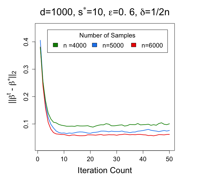
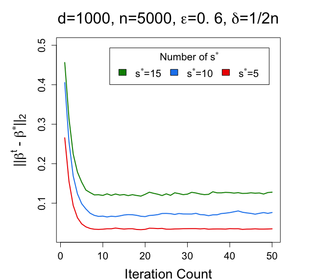
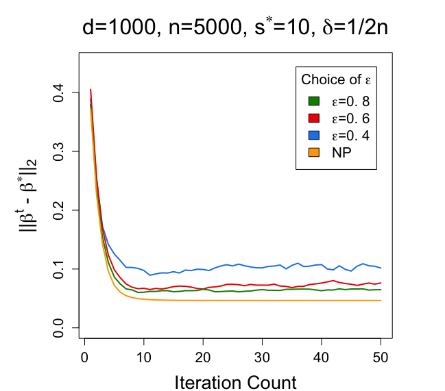
For the DP EM algorithm in the high-dimensional Gaussian mixture model, the simulated data set is constructed as follows. First, we set 𝜷\bm{\beta}^{*} to be a unit vector, where the first ss^{*} indices equal to 1/s1/\sqrt{s^{*}} and the rest of the indices are zero. For i[n]i\in[n], we generate 𝒚i=zi𝜷+𝒆i\bm{y}_{i}=z_{i}\cdot\bm{\beta}^{*}+\bm{e}_{i}, where (zi=1)=(zi=1)=1/2{\mathbb{P}}(z_{i}=1)={\mathbb{P}}(z_{i}=-1)=1/2 and 𝒆iN(0,σ2Id)\bm{e}_{i}\sim N(0,\sigma^{2}I_{d}) with σ=0.5\sigma=0.5. We consider the following three settings:

  1. 1.

    Fix d=1000,s=10,ϵ=0.5,δ=(2n)1d=1000,s^{*}=10,\epsilon=0.5,\delta=(2n)^{-1}. Compare the results of Algorithm 3 when n=4000,5000,6000n=4000,5000,6000, respectively.

  2. 2.

    Fix n=4000,d=1000,ϵ=0.5,δ=(2n)1n=4000,d=1000,\epsilon=0.5,\delta=(2n)^{-1}. Compare the results of Algorithm 3 when s=5,10,15s^{*}=5,10,15, respectively.

  3. 3.

    Fix n=4000,d=1000,s=10,δ=(2n)1n=4000,d=1000,s^{*}=10,\delta=(2n)^{-1}. Compare the results of Algorithm 3 when ϵ=0.3,0.5,0.8\epsilon=0.3,0.5,0.8, respectively.

For each setting, we repeat the experiment for 50 times and report the average of the estimation error 𝜷t𝜷2\|{\bm{\beta}}^{t}-{\bm{\beta}}^{*}\|_{2}. For each experiment, we set the step size η\eta to be 0.5. The results are plotted in Figure 1.

Refer to caption
Refer to caption
Refer to caption
Figure 1: The average estimation error under different settings in the high-dimensional Gaussian mixture model.

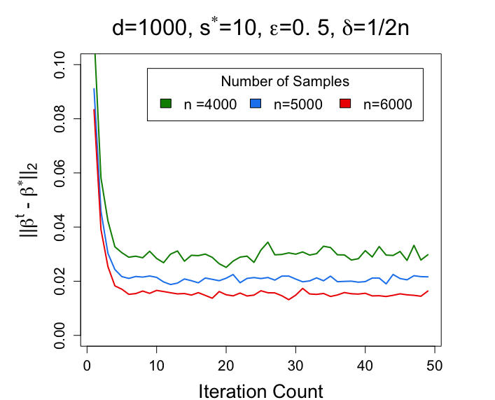
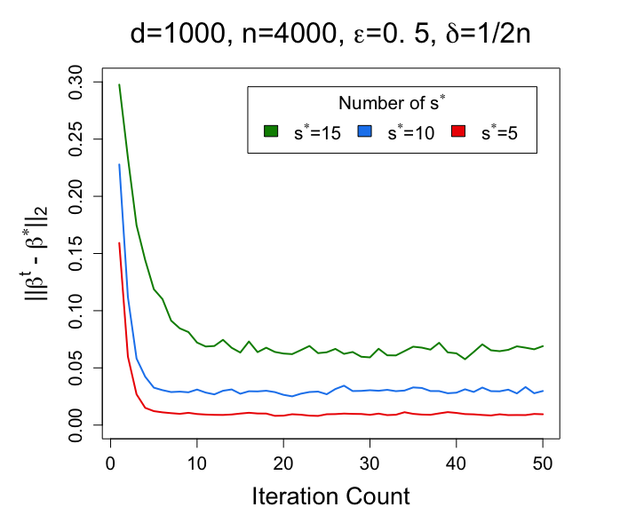
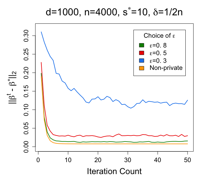
From Figure 1, we can clearly discover the relationship between different choices of n,s,ϵn,s^{*},\epsilon and the performance of proposed algorithm in the Gaussian mixture model. The left figure in Figure 1 shows that the estimation of 𝜷{\bm{\beta}}^{*} becomes more accurate when nn becomes larger. The middle figure in Figure 1 shows that when ss^{*} becomes smaller, the estimation error becomes smaller. The right figure in Figure 1 shows that when ϵ\epsilon becomes larger (the privacy constraints are more relaxed), the cost of privacy becomes smaller, and therefore the estimator achieves a smaller estimation error. With the ϵ\epsilon becomes large enough, the estimator 𝜷^\hat{{\bm{\beta}}} becomes closer to the non-private setting.

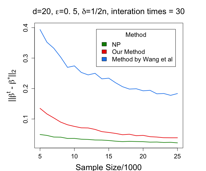
6.2 Comparison with other algorithms

In the literature, (Wang et al., 2020) also studied the DP EM algorithm in the classic low-dimensional latent variable models. In this section, we compare our proposed method with 1). the algorithm proposed in (Wang et al., 2020), and 2). the standard (non-private) gradient EM algorithm (Balakrishnan et al., 2017).

The synthetic data is generated as follows. We first set the true parameter 𝜷{\bm{\beta}}^{*} to be a unit vector with each element equal to 1/d1/\sqrt{d}. Then we simulate the Gaussian mixture model with ziz_{i} satisfying (zi=1)=(zi=1)=1/2{\mathbb{P}}(z_{i}=1)={\mathbb{P}}(z_{i}=-1)=1/2 and sample a multivariate Gaussian variable 𝒆iN(0,σ2Id)\bm{e}_{i}\sim N(0,\sigma^{2}I_{d}) with σ=0.5\sigma=0.5. At last, we compute 𝒚i=zi𝜷+𝒆i\bm{y}_{i}=z_{i}\cdot\bm{\beta}^{*}+\bm{e}_{i}.

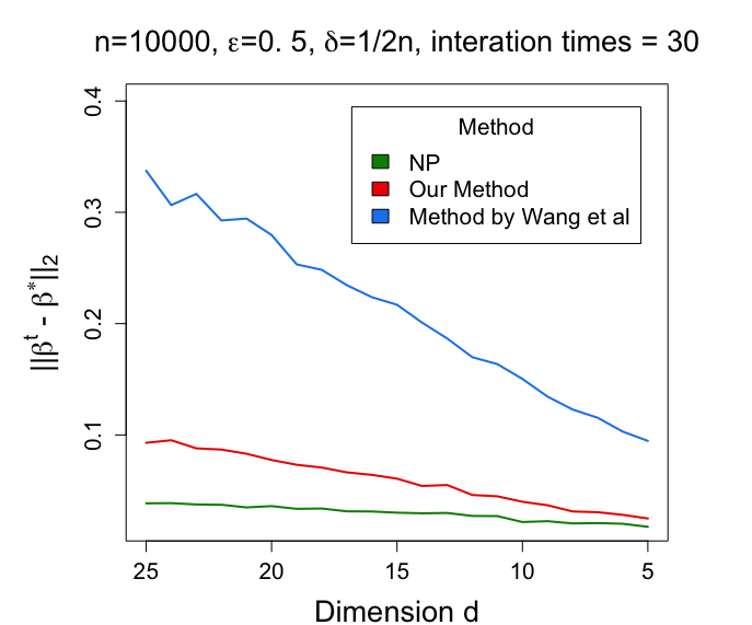
We consider the following two settings. In the first setting, we fix d,ϵ,δd,\epsilon,\delta and vary nn from 5000 to 25000; in the second setting, we fix n,ϵ,δn,\epsilon,\delta and vary dd from 5 to 25. For each setting, we report the average estimation error 𝜷𝜷^2\|{\bm{\beta}}^{*}-\hat{{\bm{\beta}}}\|_{2} among 50 repetitions. The simulation results are summarized in Figure 2. The results indicate that although there is always a gap between our algorithm with the non-private EM algorithm (due to the cost of privacy), our algorithm has a much smaller error than that produced by that in (Wang et al., 2020).

Refer to caption
Refer to caption
Figure 2: The average estimation error under different settings in the classic low-dimensional Gaussian mixture model.

6.3 Real data analysis

In this section, we apply the proposed DP EM algorithm for high-dimensional Gaussian mixture to the Breast Cancer Wisconsin (Diagnostic) Data Set, which is available at the UCI Machine Learning Repository (https://archive.ics.uci.edu/ml/datasets/Breast+Cancer+Wisconsin+(Diagnostic)) (Dua and Graff, 2017). This data set contains 569 instances and 30 attributes. Each instance describes the diagnostic result for an individual as ‘Benign’ or ‘Malignant’. In the dataset, there are 212 instances labeled as ‘Malignant’ while the rest 357 instances labeled as ‘Benign’. Such a medical diagnose data set often contains personal sensitive information and serves as a suitable data set to apply our privacy-preserving algorithms.

In our experiment, all the attributes are normalized to have zero mean and unit variance. Moreover, to make the dataset symmetric, we first randomly drop out 145 data points in the ‘Benign’ class and compute the overall sample mean. Then for each data point, we subtract the overall sample mean from it. After preprocessing, the data is randomly split into two parts, where 70% of the instances are used for training and 30% of instances are used for testing.

In the training stage, we estimate the parameter 𝜷\bm{\beta}^{*} using the proposed algorithm for high-dimensional Gaussian mixture model (Algorithm 3). We run Algorithm 3 for 50 iterations with step size η=0.5\eta=0.5. The initialization 𝜷0\bm{\beta}^{0} is chosen as the unit vector where all indexes equal 1/301/\sqrt{30}. We fix δ=1/2n\delta=1/2n, and choose various sparsity level s^\hat{s} and privacy parameter ϵ\epsilon as displayed in Table 3. In the testing stage, we classify each testing data as ‘Benign’ or ‘Malignant’ according to the 2\ell_{2} distance closeness between its attributes and 𝜷^\hat{\bm{\beta}} with the distance between its attributes and 𝜷^-\hat{\bm{\beta}}. Then we compute the misclassification rate by comparing with the true diagnostic outcome. For each choice of parameters, we repeat the whole training and testing stages for 50 times, and report the average misclassification rate and the standard error. To compare with the non-private setting, for each choice of parameters, we also use the Algorithm described in (Wang et al., 2015) as the baseline for the non-private setting (shown as ϵ=\epsilon=\infty in the table below). The results are summarized in the following Table 3.

s^=5\hat{s}=5 s^=10\hat{s}=10 s^=15\hat{s}=15
ε=0.2\varepsilon=0.2 0.14(.07) 0.12(.05) 0.10(.04)
ε=0.5\varepsilon=0.5 0.08(.02) 0.07(.02) 0.07(.01)
ε=\varepsilon=\infty 0.07(.02) 0.06(.02) 0.06(.01)
Figure 3: The average and standard error of misclassification rates of Algorithm 3 for the Breast Cancer Wisconsin Data Set.

The results suggest that when the privacy requirements become more stringent, the classification accuracy drops in a mild way. Considering the significance to achieve privacy guarantees, such loss of accuracy could be acceptable.

7 Conclusion

In this paper, we introduce a novel DP EM algorithm in both high-dimensional and low-dimensional settings. In the high-dimensional setting, we propose an algorithm based on noisy iterative hard thresholding and show this method is minimax rate-optimal up to logarithm factors in three specific models: Gaussian mixture, mixture of regression, and regression with missing covariates. In the low-dimensional setting, an algorithm based on Gaussian mechanism is also developed and shown to be near minimax optimal.

References

  • Abowd [2016] John M Abowd. The challenge of scientific reproducibility and privacy protection for statistical agencies. Census Scientific Advisory Committee, 2016.
  • Avella-Medina [2020] Marco Avella-Medina. Privacy-preserving parametric inference: a case for robust statistics. J. Am. Stat. Assoc., pages 1–15, 2020.
  • Avella-Medina et al. [2021] Marco Avella-Medina, Casey Bradshaw, and Po-Ling Loh. Differentially private inference via noisy optimization. arXiv preprint arXiv:2103.11003, 2021.
  • Awan and Slavković [2020] Jordan Awan and Aleksandra Slavković. Differentially private inference for binomial data. Journal of Privacy and Confidentiality, 10(1):1–40, 2020.
  • Bafna and Ullman [2017] Mitali Bafna and Jonathan Ullman. The price of selection in differential privacy. In COLT, pages 151–168. PMLR, 2017.
  • Balakrishnan et al. [2017] Sivaraman Balakrishnan, Martin J Wainwright, and Bin Yu. Statistical guarantees for the em algorithm: From population to sample-based analysis. Ann Stat, 45(1):77–120, 2017.
  • Bassily et al. [2014] Raef Bassily, Adam Smith, and Abhradeep Thakurta. Private empirical risk minimization: Efficient algorithms and tight error bounds. In FOCS, pages 464–473. IEEE, 2014.
  • Bun et al. [2018] Mark Bun, Jonathan Ullman, and Salil Vadhan. Fingerprinting codes and the price of approximate differential privacy. SIAM J. Comput., 47(5):1888–1938, 2018.
  • Cai et al. [2019a] T Tony Cai, Jing Ma, and Linjun Zhang. Chime: Clustering of high-dimensional gaussian mixtures with em algorithm and its optimality. Ann Stat., 47(3):1234–1267, 2019a.
  • Cai et al. [2019b] T Tony Cai, Yichen Wang, and Linjun Zhang. The cost of privacy: Optimal rates of convergence for parameter estimation with differential privacy. arXiv preprint arXiv:1902.04495, 2019b.
  • Cai et al. [2020] T Tony Cai, Yichen Wang, and Linjun Zhang. The cost of privacy in generalized linear models: Algorithms and minimax lower bounds. arXiv preprint arXiv:2011.03900, 2020.
  • Chaudhuri et al. [2013] Kamalika Chaudhuri, Anand D Sarwate, and Kaushik Sinha. A near-optimal algorithm for differentially-private principal components. J Mach Learn Res, 14, 2013.
  • Daskalakis et al. [2017] Constantinos Daskalakis, Christos Tzamos, and Manolis Zampetakis. Ten steps of em suffice for mixtures of two gaussians. In COLT, pages 704–710. PMLR, 2017.
  • Dempster et al. [1977] Arthur P Dempster, Nan M Laird, and Donald B Rubin. Maximum likelihood from incomplete data via the em algorithm. J R Stat Soc Series B, 39(1):1–22, 1977.
  • Ding et al. [2017] Bolin Ding, Janardhan Kulkarni, and Sergey Yekhanin. Collecting telemetry data privately. In NeurIPS, pages 3574–3583, 2017.
  • Ding and Song [2016] Wei Ding and Peter X-K Song. Em algorithm in gaussian copula with missing data. Comput Stat Data Anal, 101:1–11, 2016.
  • Dua and Graff [2017] Dheeru Dua and Casey Graff. UCI machine learning repository, 2017. URL http://archive.ics.uci.edu/ml.
  • Dwork and Feldman [2018] Cynthia Dwork and Vitaly Feldman. Privacy-preserving prediction. In COLT, pages 1693–1702. PMLR, 2018.
  • Dwork and Roth [2014] Cynthia Dwork and Aaron Roth. The algorithmic foundations of differential privacy. Found. Trends Theor. Comput. Sci., 9(3-4):211–407, 2014.
  • Dwork et al. [2006a] Cynthia Dwork, Krishnaram Kenthapadi, Frank McSherry, Ilya Mironov, and Moni Naor. Our data, ourselves: Privacy via distributed noise generation. In Eurocrypt, pages 486–503. Springer, 2006a.
  • Dwork et al. [2006b] Cynthia Dwork, Frank McSherry, Kobbi Nissim, and Adam Smith. Calibrating noise to sensitivity in private data analysis. In TCC, pages 265–284. Springer, 2006b.
  • Dwork et al. [2010] Cynthia Dwork, Guy N Rothblum, and Salil Vadhan. Boosting and differential privacy. In FOCS, pages 51–60. IEEE, 2010.
  • Dwork et al. [2014] Cynthia Dwork, Kunal Talwar, Abhradeep Thakurta, and Li Zhang. Analyze gauss: optimal bounds for privacy-preserving principal component analysis. In STOC, 2014.
  • Dwork et al. [2015] Cynthia Dwork, Adam Smith, Thomas Steinke, Jonathan Ullman, and Salil Vadhan. Robust traceability from trace amounts. In FOCS, pages 650–669. IEEE, 2015.
  • Dwork et al. [2017] Cynthia Dwork, Adam Smith, Thomas Steinke, and Jonathan Ullman. Exposed! a survey of attacks on private data. Annu. Rev. Stat. Appl., 4:61–84, 2017.
  • Dwork et al. [2018] Cynthia Dwork, Weijie J Su, and Li Zhang. Differentially private false discovery rate control. arXiv preprint arXiv:1807.04209, 2018.
  • Erlingsson et al. [2014] Úlfar Erlingsson, Vasyl Pihur, and Aleksandra Korolova. Rappor: Randomized aggregatable privacy-preserving ordinal response. In CCS’14, pages 1054–1067, 2014.
  • Jagannathan et al. [2009] Geetha Jagannathan, Krishnan Pillaipakkamnatt, and Rebecca N Wright. A practical differentially private random decision tree classifier. In ICDM. IEEE, 2009.
  • Kadir et al. [2014] Shabnam N Kadir, Dan FM Goodman, and Kenneth D Harris. High-dimensional cluster analysis with the masked em algorithm. Neural Comput, 26(11):2379–2394, 2014.
  • Kamath et al. [2019] Gautam Kamath, Jerry Li, Vikrant Singhal, and Jonathan Ullman. Privately learning high-dimensional distributions. In COLT, pages 1853–1902. PMLR, 2019.
  • Kamath et al. [2020a] Gautam Kamath, Or Sheffet, Vikrant Singhal, and Jonathan Ullman. Differentially private algorithms for learning mixtures of separated gaussians. In ITA, pages 1–62. IEEE, 2020a.
  • Kamath et al. [2020b] Gautam Kamath, Vikrant Singhal, and Jonathan Ullman. Private mean estimation of heavy-tailed distributions. In COLT, pages 2204–2235. PMLR, 2020b.
  • Karwa and Vadhan [2017] Vishesh Karwa and Salil Vadhan. Finite sample differentially private confidence intervals. arXiv preprint arXiv:1711.03908, 2017.
  • Kifer et al. [2020] Daniel Kifer, Solomon Messing, Aaron Roth, Abhradeep Thakurta, and Danfeng Zhang. Guidelines for implementing and auditing differentially private systems. arXiv preprint arXiv:2002.04049, 2020.
  • Kwon and Caramanis [2020] Jeongyeol Kwon and Constantine Caramanis. The EM algorithm gives sample-optimality for learning mixtures of well-separated gaussians. In COLT. PMLR, 2020.
  • Kwon et al. [2019] Jeongyeol Kwon, Wei Qian, Constantine Caramanis, Yudong Chen, and Damek Davis. Global convergence of the em algorithm for mixtures of two component linear regression. In COLT, pages 2055–2110. PMLR, 2019.
  • Kwon et al. [2020] Jeongyeol Kwon, Nhat Ho, and Constantine Caramanis. On the minimax optimality of the em algorithm for learning two-component mixed linear regression. arXiv preprint arXiv:2006.02601, 2020.
  • McLachlan and Krishnan [2007] Geoffrey J McLachlan and Thriyambakam Krishnan. The EM algorithm and extensions, volume 382. John Wiley & Sons, 2007.
  • Mirshani et al. [2019] Ardalan Mirshani, Matthew Reimherr, and Aleksandra Slavković. Formal privacy for functional data with gaussian perturbations. In ICML, pages 4595–4604. PMLR, 2019.
  • Nissim et al. [2007] Kobbi Nissim, Sofya Raskhodnikova, and Adam Smith. Smooth sensitivity and sampling in private data analysis. In STOC, pages 75–84, 2007.
  • Park et al. [2017] Mijung Park, James Foulds, Kamalika Choudhary, and Max Welling. Dp-em: Differentially private expectation maximization. In AISTATS, pages 896–904. PMLR, 2017.
  • Quost and Denoeux [2016] Benjamin Quost and Thierry Denoeux. Clustering and classification of fuzzy data using the fuzzy em algorithm. Fuzzy Sets Syst, 286:134–156, 2016.
  • Rana et al. [2015] Santu Rana, Sunil Kumar Gupta, and Svetha Venkatesh. Differentially private random forest with high utility. In ICDM2015, pages 955–960. IEEE, 2015.
  • Ranjan et al. [2016] Rishik Ranjan, Biao Huang, and Alireza Fatehi. Robust gaussian process modeling using em algorithm. J Process Control, 42:125–136, 2016.
  • Song et al. [2020] Shuang Song, Om Thakkar, and Abhradeep Thakurta. Characterizing private clipped gradient descent on convex generalized linear problems. arXiv preprint arXiv:2006.06783, 2020.
  • Song et al. [2021] Shuang Song, Thomas Steinke, Om Thakkar, and Abhradeep Thakurta. Evading the curse of dimensionality in unconstrained private glms. In AISTATS. PMLR, 2021.
  • Steinke and Ullman [2016] Thomas Steinke and Jonathan Ullman. Between pure and approximate differential privacy. Journal of Privacy and Confidentiality, 7(2):3–22, 2016.
  • Steinke and Ullman [2017] Thomas Steinke and Jonathan Ullman. Tight lower bounds for differentially private selection. In FOCS, pages 552–563. IEEE, 2017.
  • Talwar et al. [2015] Kunal Talwar, Abhradeep Thakurta, and Li Zhang. Nearly-optimal private lasso. In NeurIPS, pages 3025–3033, 2015.
  • Wang et al. [2020] Di Wang, Jiahao Ding, Zejun Xie, Miao Pan, and Jinhui Xu. Differentially private (gradient) expectation maximization algorithm with statistical guarantees. arXiv preprint arXiv:2010.13520, 2020.
  • Wang [2018] Yu-Xiang Wang. Revisiting differentially private linear regression: optimal and adaptive prediction & estimation in unbounded domain. arXiv preprint arXiv:1803.02596, 2018.
  • Wang et al. [2015] Zhaoran Wang, Quanquan Gu, Yang Ning, and Han Liu. High dimensional em algorithm: Statistical optimization and asymptotic normality. NeurIPS, 28:2512, 2015.
  • Wu [1983] CF Jeff Wu. On the convergence properties of the em algorithm. Ann Stat., pages 95–103, 1983.
  • Xu et al. [2016] Ji Xu, Daniel J Hsu, and Arian Maleki. Global analysis of expectation maximization for mixtures of two gaussians. NeurIPS, 29, 2016.
  • Yan et al. [2017] Bowei Yan, Mingzhang Yin, and Purnamrita Sarkar. Convergence of gradient em on multi-component mixture of gaussians. NeurIPS, 2017.
  • Yi and Caramanis [2015] Xinyang Yi and Constantine Caramanis. Regularized em algorithms: A unified framework and statistical guarantees. arXiv preprint arXiv:1511.08551, 2015.
  • Yi et al. [2014] Xinyang Yi, Constantine Caramanis, and Sujay Sanghavi. Alternating minimization for mixed linear regression. In ICML, pages 613–621. PMLR, 2014.
  • Zhang et al. [2020] Linjun Zhang, Rong Ma, T Tony Cai, and Hongzhe Li. Estimation, confidence intervals, and large-scale hypotheses testing for high-dimensional mixed linear regression. arXiv preprint arXiv:2011.03598, 2020.
  • Zhao et al. [2020] Ruofei Zhao, Yuanzhi Li, and Yuekai Sun. Statistical convergence of the em algorithm on gaussian mixture models. Electron. J. Stat., 14(1):632–660, 2020.
  • Zhu et al. [2017] Rongda Zhu, Lingxiao Wang, Chengxiang Zhai, and Quanquan Gu. High-dimensional variance-reduced stochastic gradient expectation-maximization algorithm. In ICML, pages 4180–4188. PMLR, 2017.

Appendix A Supplement materials

A.1 DP Algorithm and theories for Mixture of Regression Model in high-dimensional settings

By applying Algorithm 2, the DP estimation algorithm in the high-dimensional mixture of regression is presented in the following in details:

1:Private parameters (ϵ,δ)(\epsilon,\delta), step size η\eta, truncation level TT, maximum number of iterations N0N_{0}, sparsity parameter s^\hat{s}.
2:Initialization: 𝜷0\bm{\beta}^{0} with 𝜷00s^||\bm{\beta}^{0}||_{0}\leq\hat{s}.
3:For t=0,1,2,N01t=0,1,2,...N_{0}-1:
4: Compute 𝜷t+0.5=𝜷t+ηfT(Qn/N0(𝜷t;𝜷t))\bm{\beta}^{t+0.5}=\bm{\beta}^{t}+\eta\cdot f_{T}(\nabla Q_{n/N_{0}}(\bm{\beta}^{t};\bm{\beta}^{t})).
5: Let 𝜷t+1=NoisyHT(𝜷t+0.5,s^,4ηT2N0/n,ϵ,δ)\bm{\beta}^{t+1}=\text{NoisyHT}(\bm{\beta}^{t+0.5},\hat{s},4\eta\cdot T^{2}\cdot N_{0}/n,\epsilon,\delta).
16:End For
7:𝜷^=𝜷N0\hat{\bm{\beta}}=\bm{\beta}^{N_{0}}
Algorithm 5 DP Algorithm for High-Dimensional Mixture of Regression Model

For the truncation step fT(Qn(𝜷t;𝜷t))f_{T}(\nabla Q_{n}(\bm{\beta}^{t};\bm{\beta}^{t})) on line 3 of Algorithm 5, rather than using truncation on the whole gradient, we perform the truncation on yiy_{i}, 𝒙i\bm{x}_{i} and 𝒙i𝜷\bm{x}_{i}^{\top}\bm{\beta} respectively, which leads to a more refined analysis and improved rate in the statistical analysis. Specifically, we define

fT(Qn(𝜷;𝜷))=1ni=1n[2w𝜷(𝒙i,yi)ΠT(yi)ΠT(𝒙i)ΠT(𝒙i)ΠT(𝒙i𝜷)].f_{T}(\nabla Q_{n}(\bm{\beta};\bm{\beta}))=\frac{1}{n}\sum_{i=1}^{n}[2w_{\bm{\beta}}(\bm{x}_{i},y_{i})\cdot\Pi_{T}(y_{i})\cdot\Pi_{T}(\bm{x}_{i})-\Pi_{T}(\bm{x}_{i})\cdot\Pi_{T}(\bm{x}_{i}^{\top}\bm{\beta})].

Then, we could verify Conditions 3.4-3.7 in the mixture of regression model.

Lemma A.1.

Suppose we can always find a sufficiently large constant ϕ\phi to be the lower bound of the signal-to-noise ratio, 𝛃2/σ>ϕ||\bm{\beta}^{*}||_{2}/\sigma>\phi. Then

  • For Condition 3.4, Lipschitz-Gradient (γ,)(\gamma,\mathcal{B}) condition and Condition 3.5, Concavity-Smoothness (μ,ν,)(\mu,\nu,\mathcal{B}) condition, both conditions hold with the parameters

    γ(0,1/4),μ=ν=1,={𝜷:𝜷𝜷2R} with R=1/32𝜷2.\gamma\in(0,1/4),\mu=\nu=1,\mathcal{B}=\{\bm{\beta}:||\bm{\beta}-\bm{\beta}^{*}||_{2}\leq R\}\text{ with }R=1/32\cdot||\bm{\beta}^{*}||_{2}.
  • For Condition 3.6, the condition Statistical-Error(α,τ,s^,n,)(\alpha,\tau,\hat{s},n,\mathcal{B}) holds with a constant CC and

    α=Cηmax(𝜷22+σ2,1,s^𝜷2)logd+log(4/τ)n.\alpha=C\cdot\eta\cdot\max(||\bm{\beta}^{*}||_{2}^{2}+\sigma^{2},1,\sqrt{\hat{s}}\cdot||\bm{\beta}^{*}||_{2})\cdot\sqrt{\frac{\log d+\log(4/\tau)}{n}}.
  • For Condition 3.7, the condition Truncation-Error (ξ,ϕ,s^,n/N0,T,)(\xi,\phi,\hat{s},n/N_{0},T,\mathcal{B}) holds with TlognT\asymp\sqrt{\log n} and with probability 1m0/logdlogn1-m_{0}/\log d\cdot\log n, there exists a constant C1C_{1}, such that

    Qn/N0(𝜷;𝜷)fT(Qn/N0(𝜷;𝜷))2C1slogdnlogn.||\nabla Q_{n/N_{0}}(\bm{\beta};\bm{\beta})-f_{T}(\nabla Q_{n/N_{0}}(\bm{\beta};\bm{\beta}))||_{2}\leq C_{1}\cdot\sqrt{\frac{s^{*}\cdot\log d}{n}}\cdot\log n.

The detailed proof of Lemma A.1 is given in Appendix C.4.

A.2 DP Algorithm and theories for Regression with missing covariates Model in high-dimensional settings

By applying Algorithm 2, we present in the following the DP estimation in the high-dimensional regression with missing covariate model.

1:Private parameters (ϵ,δ)(\epsilon,\delta), step size η\eta, truncation level TT, maximum number of iterations N0N_{0}, sparsity parameter s^\hat{s}.
2:Initialization: 𝜷0\bm{\beta}^{0} with 𝜷00s^||\bm{\beta}^{0}||_{0}\leq\hat{s}.
3:For t=0,1,2,N01t=0,1,2,...N_{0}-1:
4: Compute 𝜷t+0.5=𝜷t+ηfT(Qn/N0(𝜷t;𝜷t))\bm{\beta}^{t+0.5}=\bm{\beta}^{t}+\eta\cdot f_{T}(Q_{n/N_{0}}(\bm{\beta}^{t};\bm{\beta}^{t})).
5: Let 𝜷t+1=NoisyHT(𝜷t+0.5,s^,6ηT2N0/n,ϵ,δ)\bm{\beta}^{t+1}=\text{NoisyHT}(\bm{\beta}^{t+0.5},\hat{s},6\eta\cdot T^{2}\cdot N_{0}/n,\epsilon,\delta).
16:End For
7:𝜷^=𝜷N0\hat{\bm{\beta}}=\bm{\beta}^{N_{0}}
Algorithm 6 DP Algorithm for High-Dim Regression with Missing Covariates

For the term fT(Qn(𝜷t;𝜷t))f_{T}(\nabla Q_{n}(\bm{\beta}^{t};\bm{\beta}^{t})) on line 3 of Algorithm 5, we design a truncation step specifically for this model. According to the definition of m𝜷(𝒙~i,yi)m_{\bm{\beta}}(\tilde{\bm{x}}_{i},y_{i}), when 𝜷\bm{\beta} is close to 𝜷\bm{\beta}^{*}, we find that m𝜷(𝒙~i,yi)m_{\bm{\beta}}(\tilde{\bm{x}}_{i},y_{i}) is close to 𝒛i𝒙i\bm{z}_{i}\odot\bm{x}_{i}, so we propose to truncate on m𝜷(𝒙~i,yi)m_{\bm{\beta}}(\tilde{\bm{x}}_{i},y_{i}) and m𝜷(𝒙~i,yi)𝜷m_{\bm{\beta}}(\tilde{\bm{x}}_{i},y_{i})^{\top}\cdot\bm{\beta}. Specifically, let

fT(Qn(𝜷;𝜷))\displaystyle f_{T}(\nabla Q_{n}(\bm{\beta};\bm{\beta})) =1ni=1n[ΠT(yi)ΠT(m𝜷(𝒙~i,yi))diag(𝟏𝒛i)𝜷\displaystyle=\frac{1}{n}\sum_{i=1}^{n}[\Pi_{T}(y_{i})\cdot\Pi_{T}(m_{\bm{\beta}}(\tilde{\bm{x}}_{i},y_{i}))-\text{diag}(\bm{1}-\bm{z}_{i})\cdot\bm{\beta}
ΠT(m𝜷(𝒙~i,yi))ΠT(m𝜷(𝒙~i,yi)𝜷)\displaystyle-\Pi_{T}(m_{\bm{\beta}}(\tilde{\bm{x}}_{i},y_{i}))\cdot\Pi_{T}(m_{\bm{\beta}}(\tilde{\bm{x}}_{i},y_{i})^{\top}\cdot\bm{\beta})
+ΠT((𝟏𝒛i)m𝜷(𝒙~i,yi))ΠT(((𝟏𝒛i)m𝜷(𝒙~i,yi))𝜷).\displaystyle+\Pi_{T}((\bm{1}-\bm{z}_{i})\odot m_{\bm{\beta}}(\tilde{\bm{x}}_{i},y_{i}))\cdot\Pi_{T}(((\bm{1}-\bm{z}_{i})\odot m_{\bm{\beta}}(\tilde{\bm{x}}_{i},y_{i}))^{\top}\cdot\bm{\beta}).

Then, we could verify Conditions 3.4-3.7 in the Regression with missing covariates model.

Lemma A.2.

Suppose the signal-to-noise ratio 𝛃2/σr||\bm{\beta}^{*}||_{2}/\sigma\leq r with r>0r>0 be some constant. Also, for the probability pp that each coordinate of 𝐱i\bm{x}_{i} is missing, we have p<1/(1+2b+2b2)p<1/(1+2b+2b^{2}) with b=r2(1+L)2b=r^{2}\cdot(1+L)^{2} and L(0,1)L\in(0,1) be a constant.

  • Condition 3.4, Lipschitz-Gradient (γ,)(\gamma,\mathcal{B}) condition and Condition 3.5, Concavity-Smoothness (μ,ν,)(\mu,\nu,\mathcal{B}) condition hold with the parameters

    γ=b+p(1+2b+2b2)1+b<1,μ=ν=1,={𝜷:𝜷𝜷2R} with R=L𝜷2.\gamma=\frac{b+p\cdot(1+2b+2b^{2})}{1+b}<1,\mu=\nu=1,\mathcal{B}=\{\bm{\beta}:||\bm{\beta}-\bm{\beta}^{*}||_{2}\leq R\}\text{ with }R=L\cdot||\bm{\beta}^{*}||_{2}.
  • For Condition 3.6, the condition Statistical-Error(α,τ,s^,n,)(\alpha,\tau,\hat{s},n,\mathcal{B}) holds with a constant CC and

    α=Cη[s^𝜷22(1+L)(1+Lr)2+max(𝜷22+σ2,(1+Lr)2)]logd+log(12/τ)n.\alpha=C\cdot\eta\cdot[\sqrt{\hat{s}}\cdot\|\bm{\beta}^{*}\|_{2}^{2}\cdot(1+L)\cdot(1+L\cdot r)^{2}+\max(||\bm{\beta}^{*}||_{2}^{2}+\sigma^{2},(1+L\cdot r)^{2})]\cdot\sqrt{\frac{\log d+\log(12/\tau)}{n}}.
  • For Condition 3.7, the condition Truncation-Error(ξ,ϕ,s^,n/N0,T,)(\xi,\phi,\hat{s},n/N_{0},T,\mathcal{B}) holds with TlognT\asymp\sqrt{\log n} and with probability 1m0/logdlogn1-m_{0}/\log d\cdot\log n, there exists a constant C1C_{1}, such that

    Qn/N0(𝜷;𝜷)fT(Qn/N0(𝜷;𝜷))2C1slogdnlogn.||\nabla Q_{n/N_{0}}(\bm{\beta};\bm{\beta})-f_{T}(\nabla Q_{n/N_{0}}(\bm{\beta};\bm{\beta}))||_{2}\leq C_{1}\cdot\sqrt{\frac{s^{*}\cdot\log d}{n}}\cdot\log n.

The detailed proof of Lemma A.2 is in the Appendix C.5.

A.3 Simulation results for mixture of regression model

For the DP EM algorithm in the high-dimensional mixture of regression model, the simulated dataset is constructed as follows. First, we set 𝜷\bm{\beta}^{*} to be a unit vector, where the first ss^{*} indices equal to 1/s1/\sqrt{s^{*}} and the rest of the indices are zero. For i[n]i\in[n], we let yi=zi𝒙i𝜷+eiy_{i}=z_{i}\cdot\bm{x}_{i}^{\top}\bm{\beta}^{*}+e_{i}, where 𝒙iN(0,𝑰d)\bm{x}_{i}\sim N(0,\bm{I}_{d}), (zi=1)=(zi=1)=1/2{\mathbb{P}}(z_{i}=1)={\mathbb{P}}(z_{i}=-1)=1/2 and eiN(0,σ2)e_{i}\sim N(0,\sigma^{2}) with σ=0.5\sigma=0.5. We consider the following three experimental settings:

  • Fix d=1000,s=10,ϵ=0.6,δ=(2n)1d=1000,s^{*}=10,\epsilon=0.6,\delta=(2n)^{-1}. Compare the results of Algorithm 5 when n=4000,5000,6000n=4000,5000,6000, respectively.

  • Fix n=5000,d=1000,ϵ=0.6,δ=(2n)1n=5000,d=1000,\epsilon=0.6,\delta=(2n)^{-1}. Compare the results of Algorithm 5 when s=5,10,15s^{*}=5,10,15, respectively.

  • Fix n=5000,d=1000,s=10,δ=(2n)1n=5000,d=1000,s^{*}=10,\delta=(2n)^{-1}. Compare the results of Algorithm 5 when ϵ=0.4,0.6,0.8\epsilon=0.4,0.6,0.8, respectively.

For each setting, we repeat the experiment for 50 times and report the average error 𝜷t𝜷2\|{\bm{\beta}}^{t}-{\bm{\beta}}^{*}\|_{2}. For each experiment, the choice of initialized 𝜷0{\bm{\beta}}^{0} should be close to the true 𝜷{\bm{\beta}}^{*} and the step size η\eta is set to be 0.5. The results are shown in Figure 4.

Refer to caption
Refer to caption
Refer to caption
Figure 4: The average estimation error under different settings under the high-dimensional mixture of regression model.

From the results in Figure 4, we also discover the relationship between different choices of n,s,ϵn,s^{*},\epsilon and the performance of the proposed DP EM algorithm on the mixture of regression model. Similar to the results under the Gaussian mixture model, with larger nn, smaller ss^{*} and larger ϵ\epsilon, the estimator 𝜷^\hat{{\bm{\beta}}} has a smaller error in estimating 𝜷{\bm{\beta}}^{*}.

A.4 Results for specific models in Low-dimensional settings

In this subsection, we will show results for DP algorithm for the mixture of regression model and regression with missing covariates in low-dimensional settings. we will list the algorithm and the theorem below. Since the proofs of these two specific models are highly similar to the proof of the high dimensional setting Theorem 4.4, Proposition 4.5, Theorem 4.6, Proposition 4.7 and also the low dimensional setting for Gaussian mixture Model Theorem 5.5 and Proposition 5.6, we omit the proofs here.

A.4.1 Algorithm and theories for Mixture of Regression Model in low-dimensional settings

The algorithm is listed as below:

3
1:Private parameters (ϵ,δ)(\epsilon,\delta), step size η\eta, truncation level TT, maximum number of iterations N0N_{0}.
2:Initialization: 𝜷0\bm{\beta}^{0}
3:For t=0,1,2,N01t=0,1,2,...N_{0}-1:
4: Compute 𝜷t+1=𝜷t+ηfT(Qn/N0(𝜷t;𝜷t))+Wt\bm{\beta}^{t+1}=\bm{\beta}^{t}+\eta f_{T}(\nabla Q_{n/N_{0}}(\bm{\beta}^{t};\bm{\beta}^{t}))+W_{t}. WtW_{t} is a random vector (ξ1,ξ2,ξd)(\xi_{1},\xi_{2},...\xi_{d})^{\top}, where ξ1,ξ2,ξd\xi_{1},\xi_{2},...\xi_{d} are i.i.d sample drawn from N(0,2η2d(4T2)2N02log(1.25/δ)n2ϵ2)N(0,\frac{2\eta^{2}d(4T^{2})^{2}{N_{0}}^{2}\log(1.25/\delta)}{n^{2}\epsilon^{2}})
15:End For
26:𝜷^=𝜷N0\hat{\bm{\beta}}=\bm{\beta}^{N_{0}}
Algorithm 7 Low Dimensional Private EM algorithm on Mixture of Regression Model

where the truncation on the gradient is the same as the truncation in Algorithm 5

Theorem A.3.

For the Algorithm 7 in the Mixture of Regression Model, we define ={𝛃:𝛃𝛃2R}\mathcal{B}=\{\bm{\beta}:||\bm{\beta}-\bm{\beta}^{*}||_{2}\leq R\} and 𝛃0𝛃2R/2||\bm{\beta}^{0}-\bm{\beta}^{*}||_{2}\leq R/2. Define R,μ,ν,γR,\mu,\nu,\gamma as in Lemma A.1 and κ=γ\kappa=\gamma. For the choice of parameters, the step size is chosen as η=1\eta=1, the truncation level is chosen as TlognT\asymp\sqrt{\log n} and the number of iterations is chosen as N0lognN_{0}\asymp\log n. For the sample size nn, it is sufficiently large that there exists constants K,KK,K^{\prime}, such that nKd(logn)32log(1/δ)(1κ)Rϵn\geq K\cdot\frac{d(\log n)^{\frac{3}{2}}\sqrt{\log(1/\delta)}}{(1-\kappa)\cdot R\cdot\epsilon} and Kdn(logn)3/2(1γ)R/4K^{\prime}\cdot\sqrt{\frac{d}{n}}\cdot(\log n)^{3/2}\leq(1-\gamma)\cdot R/4. Then, there exists sufficient large constant CC, it holds that with probability 1c0lognexp(c1d)c2/lognc3n1/21-c_{0}\log n\cdot\exp(-c_{1}d)-c_{2}/\log n-c_{3}n^{-1/2}:

𝜷^𝜷2\displaystyle||\hat{\bm{\beta}}-\bm{\beta}^{*}||_{2} Cd(logn)32log(1/δ)nϵ+η1κdn(logn)3/2.\displaystyle\leq C\cdot\frac{d\cdot(\log n)^{\frac{3}{2}}\sqrt{\log(1/\delta)}}{n\epsilon}+\frac{\eta}{1-\kappa}\cdot\sqrt{\frac{d}{n}}\cdot(\log n)^{3/2}.
Theorem A.4.

Suppose (Y,𝐗)={(y1,𝐱1),(y2,𝐱2),(yn,𝐱n)}(Y,\bm{X})=\{(y_{1},\bm{x}_{1}),(y_{2},\bm{x}_{2}),...(y_{n},\bm{x}_{n})\} be the data set of nn samples observed from the Mixture of Regression Model discussed above and let MM be any corresponding (ϵ,δ)(\epsilon,\delta)-differentially private algorithm for the estimation of the true parameter 𝛃\bm{\beta}^{*}. Then there exists a constant cc, if 0<ϵ<10<\epsilon<1 and δ<n(1+ω)\delta<n^{-(1+\omega)} for some fixed ω>0\omega>0, we have:

infMϵ,δsup𝜷d𝔼M(Y,𝑿)𝜷2c(dn+dnϵ).\inf_{M\in\mathcal{M}_{\epsilon,\delta}}\sup_{\bm{\beta}^{*}\in\mathbb{R}^{d}}\mathbb{E}\|{M(Y,\bm{X})}-\bm{\beta}^{*}\|_{2}\geq c\cdot(\sqrt{\frac{d}{n}}+\frac{d}{n\epsilon}).

A.4.2 Algorithm and theories for Regression with Missing Covariates in low dimension cases

The algorithm is listed as below:

3
1:Private parameters (ϵ,δ)(\epsilon,\delta), step size η\eta, truncation level TT, maximum number of iterations N0N_{0}.
2:Initialization: 𝜷0\bm{\beta}^{0}
3:For t=0,1,2,N01t=0,1,2,...N_{0}-1:
4: Compute 𝜷t+1=𝜷t+ηfT(Qn/N0(𝜷t;𝜷t))+Wt\bm{\beta}^{t+1}=\bm{\beta}^{t}+\eta f_{T}(\nabla Q_{n/N_{0}}(\bm{\beta}^{t};\bm{\beta}^{t}))+W_{t}. WtW_{t} is a random vector (ξ1,ξ2,ξd)(\xi_{1},\xi_{2},...\xi_{d})^{\top}, where ξ1,ξ2,ξd\xi_{1},\xi_{2},...\xi_{d} are i.i.d sample drawn from N(0,2η2d(6T2)2N02log(1.25/δ)n2ϵ2)N(0,\frac{2\eta^{2}d(6T^{2})^{2}{N_{0}}^{2}\log(1.25/\delta)}{n^{2}\epsilon^{2}})
15:End For
26:𝜷^=𝜷N0\hat{\bm{\beta}}=\bm{\beta}^{N_{0}}
Algorithm 8 Low Dimensional Private EM algorithm on Regression with missing covariates

where the truncation on the gradient is the same as the truncation in Algorithm 6

Theorem A.5.

For Algorithm 8, we define ={𝛃:𝛃𝛃2R}\mathcal{B}=\{\bm{\beta}:||\bm{\beta}-\bm{\beta}^{*}||_{2}\leq R\} and 𝛃0𝛃2R/2||\bm{\beta}^{0}-\bm{\beta}^{*}||_{2}\leq R/2. Define R,μ,ν,γR,\mu,\nu,\gamma as in Lemma A.2 and κ=γ\kappa=\gamma. For the choice of parameters, the step size is chosen as η=1\eta=1, the truncation level is chosen to be TlognT\asymp\sqrt{\log n} and the number of iterations is chosen as N0lognN_{0}\asymp\log n. For the sample size nn, it is sufficiently large that there exists constants K,KK,K^{\prime}, such that nKd(logn)32log(1/δ)(1κ)Rϵn\geq K\cdot\frac{d(\log n)^{\frac{3}{2}}\sqrt{\log(1/\delta)}}{(1-\kappa)\cdot R\cdot\epsilon} and Kdn(logn)3/2(1γ)R/4K^{\prime}\cdot\sqrt{\frac{d}{n}}\cdot(\log n)^{3/2}\leq(1-\gamma)\cdot R/4. Then, there exists sufficient large constant CC, it holds that with probability 1c0lognexp(c1d)c2/lognc3n1/21-c_{0}\log n\cdot\exp(-c_{1}d)-c_{2}/\log n-c_{3}n^{-1/2}:

𝜷^𝜷2\displaystyle||\hat{\bm{\beta}}-\bm{\beta}^{*}||_{2} Cd(logn)32log(1/δ)nϵ+η1κdn(logn)3/2.\displaystyle\leq C\cdot\frac{d\cdot(\log n)^{\frac{3}{2}}\sqrt{\log(1/\delta)}}{n\epsilon}+\frac{\eta}{1-\kappa}\cdot\sqrt{\frac{d}{n}}\cdot(\log n)^{3/2}.
Theorem A.6.

Suppose (Y,𝐗)={(y1,𝐱1),(y2,𝐱2),(yn,𝐱n)}(Y,\bm{X})=\{(y_{1},\bm{x}_{1}),(y_{2},\bm{x}_{2}),...(y_{n},\bm{x}_{n})\} be the data set of nn samples observed from the Regression with Missing covariates discussed above and let MM be any corresponding (ϵ,δ)(\epsilon,\delta)-differentially private algorithm for the estimation of the true parameter 𝛃\bm{\beta}^{*}. Then there exists a constant cc, if 0<ϵ<10<\epsilon<1 and δ<n(1+ω)\delta<n^{-(1+\omega)} for some fixed ω>0\omega>0, we have:

infMϵ,δsup𝜷d𝔼M(Y,𝑿)𝜷2c(dn+dnϵ).\inf_{M\in\mathcal{M}_{\epsilon,\delta}}\sup_{\bm{\beta}^{*}\in\mathbb{R}^{d}}\mathbb{E}\|{M(Y,\bm{X})}-\bm{\beta}^{*}\|_{2}\geq c\cdot(\sqrt{\frac{d}{n}}+\frac{d}{n\epsilon}).

Therefore, both the low-dimensioanl EM algorithm on Mixture of Regression Model and Regression with missing covariates attain a near-optimal rate of convergence up to a log factor.

Appendix B Proofs of main results

B.1 Proof of Theorem 3.8

Assume that the step size η\eta is chosen, by Lemma 3.3, we can claim the privacy is guaranteed. Then we can start the proof. For simplicity, we denote n0=n/N0n_{0}=n/N_{0}. During the tt-th iteration, we can write the iterated two steps in the following way:

𝜷t+0.5=𝜷t+ηfT(Qn0(𝜷t;𝜷t)),𝜷t+1=trunc(𝜷t+0.5,𝒮t+0.5)+𝑾Lapt.\bm{\beta}^{t+0.5}=\bm{\beta}^{t}+\eta\cdot f_{T}(\nabla Q_{n_{0}}(\bm{\beta}^{t};\bm{\beta}^{t})),\quad\bm{\beta}^{t+1}=\text{trunc}(\bm{\beta}^{t+0.5},\mathcal{S}^{t+0.5})+\bm{W}_{Lap}^{t}. (9)

where 𝒮t+0.5\mathcal{S}^{t+0.5} is the set of indices selected by the private peeling algorithm, and 𝑾Lapt\bm{W}_{Lap}^{t} is the vector of Laplace noises with support on 𝒮t+0.5\mathcal{S}^{t+0.5}. Furthermore, let us introduce the following notations, we define:

𝜷¯t+0.5=𝜷t+ηQ(𝜷t;𝜷t),𝜷¯t+1=trunc(𝜷¯t+0.5,𝒮t+0.5).\bar{\bm{\beta}}^{t+0.5}=\bm{\beta}^{t}+\eta\cdot\nabla Q(\bm{\beta}^{t};\bm{\beta}^{t}),\quad\bar{\bm{\beta}}^{t+1}=\text{trunc}(\bar{\bm{\beta}}^{t+0.5},\mathcal{S}^{t+0.5}). (10)

Then, before continue the proof, we will first introduce two lemmas:

Lemma B.1.

Suppose we have

𝜷¯t+0.5𝜷2L𝜷2,\|\bar{\bm{\beta}}^{t+0.5}-\bm{\beta}^{*}\|_{2}\leq L\|\bm{\beta}^{*}\|_{2}, (11)

for some L(0,1)L\in(0,1). Also, for the sparsity level, we have that s^4(1+L)2(1L)2s\hat{s}\geq\frac{4\cdot(1+L)^{2}}{(1-L)^{2}}\cdot s^{*} We assume that α=o(1)\alpha=o(1) and also s^α(1L)22η(1+L)𝛃2\sqrt{\hat{s}}\cdot\alpha\leq\frac{(1-L)^{2}}{2\eta(1+L)}\cdot||\bm{\beta}^{*}||_{2}. We further assume slogdn(logn)32=o(1)\frac{s^{*}\log d}{n}\cdot(\log n)^{\frac{3}{2}}=o(1). Then, it holds that, there exists a constant K1>0K_{1}>0:

𝜷¯t+1𝜷2(1+4s/s^)12𝜷¯t+0.5𝜷2+K1s1Lηα.\|\bar{\bm{\beta}}^{t+1}-\bm{\beta}^{*}\|_{2}\leq(1+4\sqrt{{s^{*}}/\hat{s}})^{\frac{1}{2}}\|\bar{\bm{\beta}}^{t+0.5}-\bm{\beta}^{*}\|_{2}+\frac{K_{1}\sqrt{s^{*}}}{\sqrt{1-L}}{\cdot\eta\cdot\alpha}. (12)

with probability 1τN0ϕ(ξ)m0slognexp(m1logd)1-\tau-N_{0}\phi(\xi)-m_{0}\cdot s^{*}\cdot\log n\cdot\exp(-m_{1}\log d), for all tt in 0,1,2,,N010,1,2,...,N_{0}-1.

Lemma B.2.

For ν\nu, μ\mu and γ\gamma defined in the Theorem 3.8, the following inequality holds:

𝜷¯t+0.5𝜷2(12νγν+μ)𝜷t𝜷2.||\bar{\bm{\beta}}^{t+0.5}-\bm{\beta}^{*}||_{2}\leq(1-2\cdot\frac{\nu-\gamma}{\nu+\mu})\cdot||{\bm{\beta}}^{t}-\bm{\beta}^{*}||_{2}. (13)

The detailed proof of Lemma B.1 is in Appendix C.6 and the proof for Lemma B.2 is in Lemma 5.2 from [Wang et al., 2015]. Then, by the two lemmas discussed above:

𝜷t+1𝜷2\displaystyle\|\bm{\beta}^{t+1}-\bm{\beta}^{*}\|_{2}
trunc(𝜷t+0.5,𝒮t+0.5)𝜷2+𝑾Lapt2\displaystyle\leq\|\text{trunc}(\bm{\beta}^{t+0.5},\mathcal{S}^{t+0.5})-\bm{\beta}^{*}\|_{2}+\|\bm{W}_{Lap}^{t}\|_{2}
trunc(𝜷t+0.5,𝒮t+0.5)trunc(𝜷¯t+0.5,𝒮t+0.5)2+trunc(𝜷¯t+0.5,𝒮t+0.5)𝜷2+𝑾Lapt2\displaystyle\leq\|\text{trunc}(\bm{\beta}^{t+0.5},\mathcal{S}^{t+0.5})-\text{trunc}(\bar{\bm{\beta}}^{t+0.5},\mathcal{S}^{t+0.5})\|_{2}+\|\text{trunc}(\bar{\bm{\beta}}^{t+0.5},\mathcal{S}^{t+0.5})-\bm{\beta}^{*}\|_{2}+\|\bm{W}_{Lap}^{t}\|_{2}
=trunc(𝜷t+0.5,St+0.5)trunc(𝜷¯t+0.5,𝒮t+0.5)2(1)+𝜷¯t+1𝜷2(2)+𝑾Lapt2.\displaystyle=\underbrace{\|\text{trunc}(\bm{\beta}^{t+0.5},S^{t+0.5})-\text{trunc}(\bar{\bm{\beta}}^{t+0.5},\mathcal{S}^{t+0.5})\|_{2}}_{(1)}+\underbrace{\|\bar{\bm{\beta}}^{t+1}-\bm{\beta}^{*}\|_{2}}_{(2)}+\|\bm{W}_{Lap}^{t}\|_{2}. (14)

First, we notice that for the term (1) in (B.1):

trunc(𝜷t+0.5,𝒮t+0.5)trunc(𝜷¯t+0.5,𝒮t+0.5)2\displaystyle\|\text{trunc}(\bm{\beta}^{t+0.5},\mathcal{S}^{t+0.5})-\text{trunc}(\bar{\bm{\beta}}^{t+0.5},\mathcal{S}^{t+0.5})\|_{2}
=(ηfT(Qn0(𝜷t;𝜷t))ηQ(𝜷t;𝜷t))𝒮t+0.5)2\displaystyle=\|(\eta f_{T}(\nabla Q_{n_{0}}(\bm{\beta}^{t};\bm{\beta}^{t}))-\eta\nabla Q(\bm{\beta}^{t};\bm{\beta}^{t}))_{\mathcal{S}^{t+0.5})}\|_{2}
(ηfT(Qn0(𝜷t;𝜷t))ηQn0(𝜷t;𝜷t))𝒮t+0.5)2+(ηQn0(𝜷t;𝜷t)ηQ(𝜷t;𝜷t))𝒮t+0.5)2\displaystyle\leq\|(\eta f_{T}(\nabla Q_{n_{0}}(\bm{\beta}^{t};\bm{\beta}^{t}))-\eta\nabla Q_{n_{0}}(\bm{\beta}^{t};\bm{\beta}^{t}))_{\mathcal{S}^{t+0.5})}\|_{2}+\|(\eta\nabla Q_{n_{0}}(\bm{\beta}^{t};\bm{\beta}^{t})-\eta\nabla Q(\bm{\beta}^{t};\bm{\beta}^{t}))_{\mathcal{S}^{t+0.5})}\|_{2}
ηfT(Qn0(𝜷t;𝜷t))Qn0(𝜷t;𝜷t)2+ηs^Qn0(𝜷t;𝜷t)Q(𝜷t;𝜷t)\displaystyle\leq\eta\|f_{T}(\nabla Q_{n_{0}}(\bm{\beta}^{t};\bm{\beta}^{t}))-\nabla Q_{n_{0}}(\bm{\beta}^{t};\bm{\beta}^{t})\|_{2}+\eta\sqrt{\hat{s}}\cdot\|\nabla Q_{n_{0}}(\bm{\beta}^{t};\bm{\beta}^{t})-\nabla Q(\bm{\beta}^{t};\bm{\beta}^{t})\|_{\infty}
ηfT(Qn0(𝜷t;𝜷t))Qn0(𝜷t;𝜷t)2+ηs^α.\displaystyle\leq\eta\|f_{T}(\nabla Q_{n_{0}}(\bm{\beta}^{t};\bm{\beta}^{t}))-\nabla Q_{n_{0}}(\bm{\beta}^{t};\bm{\beta}^{t})\|_{2}+\eta\sqrt{\hat{s}}\cdot\alpha. (15)

Second, for the term (2) in (B.1), by Lemma B.1 and Lemma B.2, we have:

𝜷¯t+1𝜷2\displaystyle{}\|\bar{\bm{\beta}}^{t+1}-\bm{\beta}^{*}\|_{2} (1+4s/s^)12𝜷¯t+0.5𝜷2+K1s1Lηα\displaystyle\leq(1+4\sqrt{{s^{*}}/\hat{s}})^{\frac{1}{2}}\|\bar{\bm{\beta}}^{t+0.5}-\bm{\beta}^{*}\|_{2}+\frac{K_{1}\sqrt{s^{*}}}{\sqrt{1-L}}{\cdot\eta\cdot\alpha}
(1+4s/s^)12(12νγν+μ)𝜷t𝜷2+K1s1Lηα.\displaystyle\leq(1+4\sqrt{{s^{*}}/\hat{s}})^{\frac{1}{2}}\cdot(1-2\cdot\frac{\nu-\gamma}{\nu+\mu})\cdot||{\bm{\beta}}^{t}-\bm{\beta}^{*}||_{2}+\frac{K_{1}\sqrt{s^{*}}}{\sqrt{1-L}}{\cdot\eta\cdot\alpha}. (16)

Third, for the term 𝑾Lapt2\|\bm{W}_{Lap}^{t}\|_{2}, notice that for any i=1,2,di=1,2,...d, {WLapt}iLaplace(λ0)\{W_{Lap}^{t}\}_{i}\sim Laplace(\lambda_{0}), by the concentration of Laplace Distribution, for every C>1C>1, we have:

(WLapt22>s^C2λ02)s^eC.{\mathbb{P}}(\|W_{Lap}^{t}\|_{2}^{2}>\hat{s}C^{2}\lambda_{0}^{2})\leq\hat{s}e^{-C}. (17)

here, in this case, λ0=Clogns^log(1/δ)/(n0ϵ)\lambda_{0}=C^{\prime}\sqrt{\log n}\sqrt{\hat{s}\log(1/\delta)}/(n_{0}\cdot\epsilon), let ClogdC\asymp\log d, we have there exists a constant C1,m2,m3C_{1},m_{2},m_{3}, such that with probability 1m2sexp(m3logd)1-m_{2}\cdot s^{*}\cdot\exp(-m_{3}\log d), we have:

𝑾Lapt22C1(slogd)2log(1/δ)lognn02ϵ2.\|\bm{W}_{Lap}^{t}\|_{2}^{2}\leq C_{1}\cdot\frac{(s^{*}\log d)^{2}\log(1/\delta)\log n}{n_{0}^{2}\epsilon^{2}}. (18)

By a union bound and the choice of N0N_{0} to be N0lognN_{0}\asymp\log n, we find that with probability 1m2slognexp(m3logd)1-m_{2}\cdot s^{*}\cdot\log n\cdot\exp(-m_{3}\log d), we have:

maxt𝑾Lapt22C1(slogd)2log(1/δ)lognn02ϵ2.\max_{t}\|\bm{W}_{Lap}^{t}\|_{2}^{2}\leq C_{1}\cdot\frac{(s^{*}\log d)^{2}\log(1/\delta)\log n}{n_{0}^{2}\epsilon^{2}}. (19)

According to our assumption, we find that 𝑾Lapt2\|\bm{W}_{Lap}^{t}\|_{2} is o(1). Thus, by combining the results from (B.1)(B.1)(B.1), we find that:

𝜷t+1𝜷2\displaystyle\|\bm{\beta}^{t+1}-\bm{\beta}^{*}\|_{2} ηs^α+(1+4s/s^)12(12νγν+μ)𝜷t𝜷2+K1s1Lηα\displaystyle\leq\eta\sqrt{\hat{s}}\cdot\alpha+(1+4\sqrt{{s^{*}}/\hat{s}})^{\frac{1}{2}}\cdot(1-2\cdot\frac{\nu-\gamma}{\nu+\mu})\cdot||{\bm{\beta}}^{t}-\bm{\beta}^{*}||_{2}+\frac{K_{1}\sqrt{s^{*}}}{\sqrt{1-L}}{\cdot\eta\cdot\alpha}
+ηfT(Qn0(𝜷t;𝜷t))Qn0(𝜷t;𝜷t)2+𝑾Lapt2.\displaystyle+\eta\|f_{T}(\nabla Q_{n_{0}}(\bm{\beta}^{t};\bm{\beta}^{t}))-\nabla Q_{n_{0}}(\bm{\beta}^{t};\bm{\beta}^{t})\|_{2}+\|\bm{W}_{Lap}^{t}\|_{2}. (20)

Denote κ=12νγν+μ\kappa=1-2\cdot\frac{\nu-\gamma}{\nu+\mu}. Then, if βt\beta^{t}\in\mathcal{B}, by our assumption in the theorem that s^16(1/κ1)2s\hat{s}\geq 16\cdot(1/\kappa-1)^{-2}\cdot s^{*}, we have (1+4s/s^)1/21/κ(1+4\cdot\sqrt{s^{*}/\hat{s}})^{1/2}\leq 1/\sqrt{\kappa}. thus we have (1+4s/s^)12(12νγν+μ)κ(1+4\sqrt{{s^{*}}/\hat{s}})^{\frac{1}{2}}\cdot(1-2\cdot\frac{\nu-\gamma}{\nu+\mu})\leq\sqrt{\kappa}.

On the other hand, we find that by the assumption we also have (s^+K1s1L)ηα(1κ)2R(\sqrt{\hat{s}}+\frac{K_{1}\sqrt{s^{*}}}{\sqrt{1-L}})\cdot\eta\cdot\alpha\leq(1-\sqrt{\kappa})^{2}\cdot R. Further more, by the assumptions, we also have thatWLapt2\|W_{Lap}^{t}\|_{2} are o(1)o(1) for any tt, and with probability 1N0ϕ(ξ)1-N_{0}\cdot\phi(\xi), maxtfT(Qn0(𝜷t;𝜷t))Qn0(𝜷t;𝜷t)2<ξ\max_{t}\|f_{T}(\nabla Q_{n_{0}}(\bm{\beta}^{t};\bm{\beta}^{t}))-\nabla Q_{n_{0}}(\bm{\beta}^{t};\bm{\beta}^{t})\|_{2}<\xi where ξ=o(1)\xi=o(1).

𝜷t+1𝜷2(1κ)2R+κRR,\displaystyle\|\bm{\beta}^{t+1}-\bm{\beta}^{*}\|_{2}\leq(1-\sqrt{\kappa})^{2}R+\sqrt{\kappa}R\leq R, (21)

which guarantees that if 𝜷t\bm{\beta}^{t}\in\mathcal{B}, we also have 𝜷t+1\bm{\beta}^{t+1}\in\mathcal{B}. Iterate this, we can get the connection between 𝜷t𝜷2\|\bm{\beta}^{t}-\bm{\beta}^{*}\|_{2} and 𝜷0𝜷2\|\bm{\beta}^{0}-\bm{\beta}^{*}\|_{2}:

𝜷t𝜷2\displaystyle\|\bm{\beta}^{t}-\bm{\beta}^{*}\|_{2} (s^+K1/1Ls)η1κα+κt/2𝜷t𝜷2\displaystyle\leq\frac{(\sqrt{\hat{s}}+K_{1}/\sqrt{1-L}\cdot\sqrt{s^{*}})\cdot\eta}{1-\sqrt{\kappa}}\cdot\alpha+\kappa^{t/2}\cdot||{\bm{\beta}}^{t}-\bm{\beta}^{*}||_{2}
+ηξ/(1κ)+K2slogdlog(1/δ)(logn)3/2nϵ,\displaystyle+\eta\cdot\xi/(1-\sqrt{\kappa})+K_{2}\cdot\frac{s^{*}\log d\cdot\sqrt{\log(1/\delta)}(\log n)^{3/2}}{n\epsilon}, (22)

which finishes the proof for the theorem. \square

B.2 Proof of Theorem 4.2

The proof of theorem 4.2 consists of three parts. The first part is the privacy guarantees. The second part is to verify the conditions for α\alpha is satisfied. The third part is to find the convergence rate of Qn/N0(𝜷;𝜷)fT(Qn/N0(𝜷;𝜷))2||\nabla Q_{n/N_{0}}(\bm{\beta};\bm{\beta})-f_{T}(\nabla Q_{n/N_{0}}(\bm{\beta};\bm{\beta}))||_{2}, for any 𝜷\bm{\beta} on the iteration path. Let us begin the proof with the first part.

For the privacy guarantee, notice that for two adjacent data sets, let yiy_{i} and yi{y_{i}}^{\prime} be the difference between these two data sets.

fT(Qn/N0(𝜷;𝜷))fT(Qn/N0(𝜷;𝜷))\displaystyle||f_{T}(\nabla Q_{n/N_{0}}(\bm{\beta};\bm{\beta}))-f_{T}(\nabla{Q_{n/N_{0}}}^{\prime}(\bm{\beta};\bm{\beta}))||_{\infty}
=N0n[2w𝜷(yi)1]ΠT(yi)N0n[2w𝜷(yi)1]ΠT(yi)\displaystyle=||\frac{N_{0}}{n}\cdot[2w_{\bm{\beta}}(y_{i})-1]\cdot\Pi_{T}(y_{i})-\frac{N_{0}}{n}\cdot[2w_{\bm{\beta}}({y_{i}}^{\prime})-1]\cdot\Pi_{T}({y_{i}}^{\prime})||_{\infty}
N0n[ΠT(yi)+ΠT(yi)]\displaystyle\leq\frac{N_{0}}{n}\cdot[||\Pi_{T}(y_{i})||_{\infty}+||\Pi_{T}({y_{i}}^{\prime})||_{\infty}]
2TN0n.\displaystyle\leq\frac{2T\cdot N_{0}}{n}. (23)

Then, by Lemma 3.3, we can claim that the private Gaussian Mixture Model is (ϵ,δ)(\epsilon,\delta)-differentially private.

Also, for the conditions of α\alpha is Theorem 3.8, we find that (s^+c1/1Ls)ηα(\sqrt{\hat{s}}+c_{1}/\sqrt{1-L}\cdot\sqrt{s^{*}})\cdot\eta\cdot\alpha is roughly O(slogdlogn/n)O(\sqrt{s^{*}\cdot\log d\cdot\log n/n}) and also by the assumption that slogdn(logn)52=o(1)\frac{s^{*}\log d}{n}\cdot(\log n)^{\frac{5}{2}}=o(1), we can claim that (s^+c1/1Ls)ηα(\sqrt{\hat{s}}+c_{1}/\sqrt{1-L}\cdot\sqrt{s^{*}})\cdot\eta\cdot\alpha is actually o(1)o(1), thus the condition (s^+c1/1Ls^)ηαmin((1κ)2R,(1L)22(1+L)𝜷2)(\sqrt{\hat{s}}+c_{1}/\sqrt{1-L}\cdot\hat{s^{*}})\cdot\eta\cdot\alpha\leq\min((1-\sqrt{\kappa})^{2}\cdot R,\frac{(1-L)^{2}}{2\cdot(1+L)}\cdot\|\bm{\beta}^{*}\|_{2}) can be satisfied. Therefore, we can find a constant CC, such that:

(s^+c1/1Ls)η1καCslogdlognn.\frac{(\sqrt{\hat{s}}+c_{1}/\sqrt{1-L}\cdot\sqrt{s^{*}})\cdot\eta}{1-\sqrt{\kappa}}\cdot\alpha\leq C\cdot\sqrt{\frac{s^{*}\cdot\log d\cdot\log n}{n}}. (24)

Then, to finish the proof, it suffices to show that for each 𝜷t\bm{\beta}^{t}, t=0,1,2,N01t=0,1,2,...N_{0}-1, we can claim Qn/N0(𝜷t;𝜷t)fT(Qn/N0(𝜷t;𝜷t))2||\nabla Q_{n/N_{0}}(\bm{\beta}^{t};\bm{\beta}^{t})-f_{T}(\nabla Q_{n/N_{0}}(\bm{\beta}^{t};\bm{\beta}^{t}))||_{2} is O(slogdlognn)O(\sqrt{\frac{s^{*}\cdot\log d\cdot\log n}{n}}). Then we can follow the proof of Theorem 3.8 to finish the proof of Theorem 4.2.

By the third proposition in Lemma 4.1, we have already observed that for any t=0,1,2,,N01t=0,1,2,\cdots,N_{0}-1, if we choose ξ=O(slogdlognn)\xi=O(\sqrt{\frac{s^{*}\cdot\log d\cdot\log n}{n}}). We can find that for a constant CC^{\prime}:

P(Qn/N0(𝜷t;𝜷t)fT(Qn/N0(𝜷t;𝜷t))2>ξ)C1logdlogn.P(||\nabla Q_{n/N_{0}}(\bm{\beta}^{t};\bm{\beta}^{t})-f_{T}(\nabla Q_{n/N_{0}}(\bm{\beta}^{t};\bm{\beta}^{t}))||_{2}>\xi)\leq C^{\prime}\cdot\frac{1}{\log d\cdot\log n}.

Furthermore, for all t=0,1,N01t=0,1,...N_{0}-1, since N0N_{0} is chosen to be O(logn)O(\log n), we could apply an union bound, and claim that for all tt, with probability 1Clogd1-C^{\prime}\log d, Qn/N0(𝜷t;𝜷t)fT(Qn/N0(𝜷t;𝜷t))2=O(slogdlognn)||\nabla Q_{n/N_{0}}(\bm{\beta}^{t};\bm{\beta}^{t})-f_{T}(\nabla Q_{n/N_{0}}(\bm{\beta}^{t};\bm{\beta}^{t}))||_{2}=O(\sqrt{\frac{s^{*}\cdot\log d\cdot\log n}{n}}), which finishes the proof of Theorem 4.2. \square

B.3 Proof of Proposition 4.3

Suppose 𝒀={𝒚1,𝒚2,𝒚n}\bm{Y}=\{\bm{y}_{1},\bm{y}_{2},...\bm{y}_{n}\} be the data set of nn samples observed from the Gaussian Mixture Model and let MM be any corresponding (ϵ,δ)(\epsilon,\delta)-differentially private algorithm. Suppose we have another model where there are no hidden variables ZZ where 𝒀=β+𝒆\bm{Y}=\beta^{*}+\bm{e}. Suppose 𝒀1={𝒚1,𝒚2,𝒚n}\bm{Y}_{1}=\{\bm{y}_{1}^{\prime},\bm{y}_{2}^{\prime},...\bm{y}_{n}^{\prime}\} be the data set of nn samples observed from the latter model and let M1M_{1} be any corresponding (ϵ,δ)(\epsilon,\delta)-differentially private algorithm. Then the estimation of true 𝜷\bm{\beta}^{*} can be seen as a mean-estimation problem. By Lemma 3.2 and Theorem 3.3 from [Cai et al., 2019b], we have that:

infM1ϵ,δsup𝜷d,𝜷0s𝔼M1(𝒀1)𝜷2c(slogdn+slogdnϵ)\inf_{M_{1}\in\mathcal{M}_{\epsilon,\delta}}\sup_{\bm{\beta}^{*}\in\mathbb{R}^{d},\|\bm{\beta}^{*}\|_{0}\leq s^{*}}\mathbb{E}\|{M_{1}(\bm{Y}_{1})}-\bm{\beta}^{*}\|_{2}\geq c\cdot(\sqrt{\frac{s^{*}\log d}{n}}+\frac{s^{*}\log d}{n\epsilon})

Since the no hidden variables model can be seen as a special case where all hidden variables ZZ equals 1, so we have:

infM0ϵ,δsup𝜷d,𝜷0s𝔼M(𝒀)𝜷2infM1ϵ,δsup𝜷d,𝜷0s𝔼M1(𝒀1)𝜷2\inf_{M_{0}\in\mathcal{M}_{\epsilon,\delta}}\sup_{\bm{\beta}^{*}\in\mathbb{R}^{d},\|\bm{\beta}^{*}\|_{0}\leq s^{*}}\mathbb{E}\|{M(\bm{Y})}-\bm{\beta}^{*}\|_{2}\geq\inf_{M_{1}\in\mathcal{M}_{\epsilon,\delta}}\sup_{\bm{\beta}^{*}\in\mathbb{R}^{d},\|\bm{\beta}^{*}\|_{0}\leq s^{*}}\mathbb{E}\|{M_{1}(\bm{Y}_{1})}-\bm{\beta}^{*}\|_{2}

By combining the two inequalities together, we finish the proof. \square

B.4 Proof of Theorem 4.4

Similar to the proof for Theorem 4.2, the proof consists of three parts. The first part is the privacy guarantees. The second part is to verify the conditions of α\alpha. The third part is to find the convergence of maxtQn/N0(𝜷t;𝜷t)fT(Qn/N0(𝜷t;𝜷t))2\max_{t}||\nabla Q_{n/N_{0}}(\bm{\beta}^{t};\bm{\beta}^{t})-f_{T}(\nabla Q_{n/N_{0}}(\bm{\beta}^{t};\bm{\beta}^{t}))||_{2}. Here, the verification of α\alpha is similar to the proof of Theorem 4.2, so we omit the proof here.

For the privacy guarantee, notice that for two adjacent data sets, let (𝒙i,yi)(\bm{x}_{i},y_{i}) and (𝒙i,yi)(\bm{x}_{i}^{\prime},y_{i}^{\prime}) be the difference between these two data sets.

fT(Qn/N0(𝜷;𝜷))fT(Qn/N0(𝜷;𝜷))\displaystyle||f_{T}(\nabla Q_{n/N_{0}}(\bm{\beta};\bm{\beta}))-f_{T}(\nabla{Q_{n/N_{0}}^{\prime}}(\bm{\beta};\bm{\beta}))||_{\infty}
=||N0n[2w𝜷(𝒙i,yi)ΠT(yi)ΠT(𝒙i)ΠT(𝒙i)ΠT(𝒙i𝜷)]\displaystyle=||\frac{N_{0}}{n}\cdot[2w_{\bm{\beta}}(\bm{x}_{i},y_{i})\cdot\Pi_{T}(y_{i})\cdot\Pi_{T}(\bm{x}_{i})-\Pi_{T}(\bm{x}_{i})\cdot\Pi_{T}(\bm{x}_{i}^{\top}\bm{\beta})]
N0n[2w𝜷(𝒙i,yi)ΠT(yi)ΠT(𝒙i)ΠT(𝒙i)ΠT(𝒙𝒊𝜷)]||\displaystyle-\frac{N_{0}}{n}\cdot[2w_{\bm{\beta}}(\bm{x}_{i}^{\prime},y_{i}^{\prime})\cdot\Pi_{T}(y_{i}^{\prime})\cdot\Pi_{T}(\bm{x}_{i}^{\prime})-\Pi_{T}(\bm{x}_{i}^{\prime})\cdot\Pi_{T}(\bm{x_{i}^{\prime}}^{\top}\bm{\beta})]||_{\infty}
N0nΠT(yi)ΠT(𝒙i)ΠT(yi)ΠT(𝒙i)+N0nΠT(𝒙i)ΠT(𝒙i𝜷)ΠT(𝒙i)ΠT(𝒙𝒊𝜷)\displaystyle\leq\frac{N_{0}}{n}\|\Pi_{T}(y_{i})\cdot\Pi_{T}(\bm{x}_{i})-\Pi_{T}(y_{i}^{\prime})\cdot\Pi_{T}(\bm{x}_{i}^{\prime})\|_{\infty}+\frac{N_{0}}{n}\|\Pi_{T}(\bm{x}_{i})\cdot\Pi_{T}(\bm{x}_{i}^{\top}\bm{\beta})-\Pi_{T}(\bm{x}_{i}^{\prime})\cdot\Pi_{T}(\bm{x_{i}^{\prime}}^{\top}\bm{\beta})\|_{\infty}
4T2N0n.\displaystyle\leq\frac{4T^{2}\cdot N_{0}}{n}. (25)

Next, let us find the convergence rate for the truncation error. By Lemma A.1, for the truncation error, we have obtained that with probability 1m0/(lognlogd)1-m_{0}/(\log n\cdot\log d), therefore, for any t=0,1,2,,N01t=0,1,2,...,N_{0}-1, we have:

(Qn0(𝜷t;𝜷t)fT(Qn0(𝜷t;𝜷t))2>Cslogdnlogn)C1/logdlogn,{\mathbb{P}}(||\nabla Q_{n_{0}}(\bm{\beta}^{t};\bm{\beta}^{t})-f_{T}(\nabla Q_{n_{0}}(\bm{\beta}^{t};\bm{\beta}^{t}))||_{2}>C\cdot\sqrt{\frac{s^{*}\log d}{n}}\cdot\log n)\leq C^{\prime}\cdot 1/{\log d\cdot\log n}, (26)

By a union bound on tt, and if we take the times of iteration N0lognN_{0}\asymp\log n, we have:

(maxtQn0(𝜷t;𝜷t)fT(Qn0(𝜷t;𝜷t))2>Cslogdnlogn)C1/logd.{\mathbb{P}}(\max_{t}||\nabla Q_{n_{0}}(\bm{\beta}^{t};\bm{\beta}^{t})-f_{T}(\nabla Q_{n_{0}}(\bm{\beta}^{t};\bm{\beta}^{t}))||_{2}>C\cdot\sqrt{\frac{s^{*}\log d}{n}}\cdot\log n)\leq C^{\prime}\cdot 1/{\log d}. (27)

Thus, we can get the result that for all tt, with probability 1C/logd1-C^{\prime}/{\log d}, Qn/N0(𝜷t;𝜷t)fT(Qn/N0(𝜷t;𝜷t))2=O(slogdnlogn)||\nabla Q_{n/N_{0}}(\bm{\beta}^{t};\bm{\beta}^{t})-f_{T}(\nabla Q_{n/N_{0}}(\bm{\beta}^{t};\bm{\beta}^{t}))||_{2}=O(\sqrt{\frac{s^{*}\log d}{n}}\cdot\log n), thus follows the proof of Theorem 3.8, we finish the proof of Theorem 4.4. \square

B.5 Proof of Proposition 4.5

Suppose we have the traditional linear regression model where there are no hidden variables ZZ where Y=𝑿β+𝒆Y=\bm{X}^{\top}\beta^{*}+\bm{e}. Suppose (Y1,𝑿1)={(y1,𝒙1),(y2,𝒙2),(yn,𝒙n)}(Y_{1},\bm{X}_{1})=\{(y_{1}^{\prime},\bm{x}_{1}^{\prime}),(y_{2}^{\prime},\bm{x}_{2}^{\prime}),...(y_{n}^{\prime},\bm{x}_{n}^{\prime})\} be the data set of nn samples observed from the linear regression model and let M1M_{1} be any corresponding (ϵ,δ)(\epsilon,\delta)-differentially private algorithm. Then by Lemma 4.3 and Theorem 4.3 in [Cai et al., 2019b], we have that:

infM1ϵ,δsup𝜷d,𝜷0s𝔼M1(Y1,𝑿1)𝜷2c(slogdn+slogdnϵ).\inf_{M_{1}\in\mathcal{M}_{\epsilon,\delta}}\sup_{\bm{\beta}^{*}\in\mathbb{R}^{d},\|\bm{\beta}^{*}\|_{0}\leq s^{*}}\mathbb{E}\|{M_{1}(Y_{1},\bm{X}_{1})}-\bm{\beta}^{*}\|_{2}\geq c\cdot(\sqrt{\frac{s^{*}\log d}{n}}+\frac{s^{*}\log d}{n\epsilon}).

Since the no hidden variables model can be seen as a special case where all hidden variables ZZ equals 1, so we have:

infMϵ,δsup𝜷d,𝜷0s𝔼M(Y,𝑿)𝜷2infM1ϵ,δsup𝜷d,𝜷0s𝔼M1(Y1,𝑿1)𝜷2.\inf_{M\in\mathcal{M}_{\epsilon,\delta}}\sup_{\bm{\beta}^{*}\in\mathbb{R}^{d},\|\bm{\beta}^{*}\|_{0}\leq s^{*}}\mathbb{E}\|{M(Y,\bm{X})}-\bm{\beta}^{*}\|_{2}\geq\inf_{M_{1}\in\mathcal{M}_{\epsilon,\delta}}\sup_{\bm{\beta}^{*}\in\mathbb{R}^{d},\|\bm{\beta}^{*}\|_{0}\leq s^{*}}\mathbb{E}\|{M_{1}(Y_{1},\bm{X}_{1})}-\bm{\beta}^{*}\|_{2}.

By combining the two inequalities together, we finish the proof. \square

B.6 Proof of Theorem 4.6

In the proof of Theorem 4.6, we also need to verify two properties. First is the privacy guarantees. The second part is to find the convergence of maxtQn/N0(𝜷t;𝜷t)fT(Qn/N0(𝜷t;𝜷t))2\max_{t}||\nabla Q_{n/N_{0}}(\bm{\beta}^{t};\bm{\beta}^{t})-f_{T}(\nabla Q_{n/N_{0}}(\bm{\beta}^{t};\bm{\beta}^{t}))||_{2}.

For the privacy guarantee, notice that for two adjacent data sets, let (𝒙i,yi)(\bm{x}_{i},y_{i}) and (𝒙i,yi)(\bm{x}_{i}^{\prime},y_{i}^{\prime}) be the difference between these two data sets. For the ease of notation, we denote n𝜷(𝒙~i,yi,zi))=(1𝒛i)m𝜷(𝒙~i,yi))n_{\bm{\beta}}(\tilde{\bm{x}}_{i},y_{i},z_{i}))=(1-\bm{z}_{i})\odot m_{\bm{\beta}}(\tilde{\bm{x}}_{i},y_{i})) and ui=(1𝒛i)m𝜷(𝒙~i,yi)𝜷u_{i}=(1-\bm{z}_{i})\odot m_{\bm{\beta}}(\tilde{\bm{x}}_{i},y_{i})^{\top}\cdot\bm{\beta}. Then:

fT(Qn/N0(𝜷;𝜷))fT(Qn/N0(𝜷;𝜷))\displaystyle||f_{T}(\nabla Q_{n/N_{0}}(\bm{\beta};\bm{\beta}))-f_{T}(\nabla{Q_{n/N_{0}}^{\prime}}(\bm{\beta};\bm{\beta}))||_{\infty}
N0nΠT(yi)ΠT(mβ(𝒙~i,yi))ΠT(yi)ΠT(mβ(𝒙~i,yi))\displaystyle\leq\frac{N_{0}}{n}||\Pi_{T}(y_{i})\cdot\Pi_{T}(m_{\beta}(\tilde{\bm{x}}_{i},y_{i}))-\Pi_{T}(y_{i}^{\prime})\cdot\Pi_{T}(m_{\beta}(\tilde{\bm{x}}_{i}^{\prime},y_{i}^{\prime}))||_{\infty}
+N0nΠT(m𝜷(𝒙~i,yi))ΠT(m𝜷(𝒙~i,yi)𝜷)ΠT(m𝜷(𝒙~i,yi))ΠT(m𝜷(𝒙~i,yi)𝜷)\displaystyle+\frac{N_{0}}{n}||\Pi_{T}(m_{\bm{\beta}}(\tilde{\bm{x}}_{i},y_{i}))\cdot\Pi_{T}(m_{\bm{\beta}}(\tilde{\bm{x}}_{i},y_{i})^{\top}\cdot\bm{\beta})-\Pi_{T}(m_{\bm{\beta}}(\tilde{\bm{x}}_{i}^{\prime},y_{i}^{\prime}))\cdot\Pi_{T}(m_{\bm{\beta}}(\tilde{\bm{x}}_{i}^{\prime},y_{i}^{\prime})^{\top}\cdot\bm{\beta})||_{\infty}
+N0nΠT(n𝜷(𝒙~i,yi,zi))ΠT(ui)ΠT(n𝜷(𝒙~i,yi,zi))ΠT(ui)\displaystyle+\frac{N_{0}}{n}||\Pi_{T}(n_{\bm{\beta}}(\tilde{\bm{x}}_{i},y_{i},z_{i}))\cdot\Pi_{T}(u_{i})-\Pi_{T}(n_{\bm{\beta}}(\tilde{\bm{x}}_{i}^{\prime},y_{i}^{\prime},z_{i}^{\prime}))\cdot\Pi_{T}(u_{i}^{\prime})||_{\infty}
6T2N0n\displaystyle\leq\frac{6T^{2}\cdot N_{0}}{n} (28)

From Lemma A.2, we have that under the truncation condition, with probability 1m0/(lognlogd)1-m_{0}/(\log n\cdot\log d), for any t=0,1,2,,N01t=0,1,2,...,N_{0}-1, we have:

P(Qn/N0(𝜷t;𝜷t)fT(Qn/N0(𝜷t;𝜷t))2>Cslogdnlogn)C1/logdlogn,P(||\nabla Q_{n/N_{0}}(\bm{\beta}^{t};\bm{\beta}^{t})-f_{T}(\nabla Q_{n/N_{0}}(\bm{\beta}^{t};\bm{\beta}^{t}))||_{2}>C\cdot\sqrt{\frac{s^{*}\log d}{n}}\cdot\log n)\leq C^{\prime}\cdot 1/{\log d\cdot\log n}, (29)

Again, by a union bound on tt, and if we take the times of iteration N0lognN_{0}\asymp\log n, we have:

P(maxtQn/N0(𝜷t;𝜷t)fT(Qn/N0(𝜷t;𝜷t))2>Cslogdnlogn)C1/logdP(\max_{t}||\nabla Q_{n/N_{0}}(\bm{\beta}^{t};\bm{\beta}^{t})-f_{T}(\nabla Q_{n/N_{0}}(\bm{\beta}^{t};\bm{\beta}^{t}))||_{2}>C\cdot\sqrt{\frac{s^{*}\log d}{n}}\cdot\log n)\leq C^{\prime}\cdot 1/{\log d} (30)

Thus, we can get the result that for all tt, with probability 1C/logd1-C^{\prime}/{\log d}, maxtQn/N0(𝜷t;𝜷t)fT(Qn/N0(𝜷t;𝜷t))2=O(slogdnlogn)\max_{t}||\nabla Q_{n/N_{0}}(\bm{\beta}^{t};\bm{\beta}^{t})-f_{T}(\nabla Q_{n/N_{0}}(\bm{\beta}^{t};\bm{\beta}^{t}))||_{2}=O(\sqrt{\frac{s^{*}\log d}{n}}\cdot\log n), thus by Theorem 3.8, we finish the proof of Theorem 4.6. \square

B.7 Proof of Theorem 5.4

Before the proof, let us first introduce a lemma:

Lemma B.3.

If 0γ<νμ0\leq\gamma<\nu\leq\mu holds, suppose that Condition 3.4, 3.5 holds with parameter γ,(μ,ν)\gamma,(\mu,\nu), respectively. Then if step size η=2μ+ν\eta=\frac{2}{\mu+\nu}, we have:

𝜷+ηQ(𝜷;𝜷)𝜷2(12ν2γμ+ν)𝜷𝜷2.\displaystyle||\bm{\beta}+\eta\cdot\nabla{Q(\bm{\beta};\bm{\beta})}-\bm{\beta}^{*}||_{2}\leq(1-\frac{2\nu-2\gamma}{\mu+\nu})||\bm{\beta}-\bm{\beta}^{*}||_{2}.

The detailed proof for B.3 is in Theorem 3 from [Balakrishnan et al., 2017]. Then for t=0,1,2,3,N01t=0,1,2,3,...N_{0}-1, we have:

𝜷t+1𝜷2\displaystyle||\bm{\beta}^{t+1}-\bm{\beta}^{*}||_{2} =𝜷t+ηfT(Qn/N0(𝜷t;𝜷t))+𝑾t𝜷2\displaystyle=||\bm{\beta}^{t}+\eta f_{T}(\nabla Q_{n/N_{0}}(\bm{\beta}^{t};\bm{\beta}^{t}))+\bm{W}_{t}-\bm{\beta}^{*}||_{2}
𝜷t+ηQ(𝜷t;𝜷t)𝜷2+ηfT(Qn/N0(𝜷t;𝜷t))Q(𝜷t;𝜷t)2+𝑾t2\displaystyle\leq||\bm{\beta}^{t}+\eta\nabla Q(\bm{\beta}^{t};\bm{\beta}^{t})-\bm{\beta}^{*}||_{2}+\eta||f_{T}(\nabla Q_{n/N_{0}}(\bm{\beta}^{t};\bm{\beta}^{t}))-\nabla Q(\bm{\beta}^{t};\bm{\beta}^{t})||_{2}+||\bm{W}_{t}||_{2}
κ𝜷t𝜷2+𝑾t2+ηfT(Qn/N0(𝜷t;𝜷t))Qn/N0(𝜷t;𝜷t)2\displaystyle\leq\kappa||\bm{\beta}^{t}-\bm{\beta}^{*}||_{2}+||\bm{W}_{t}||_{2}+\eta||f_{T}(\nabla Q_{n/N_{0}}(\bm{\beta}^{t};\bm{\beta}^{t}))-\nabla Q_{n/N_{0}}(\bm{\beta}^{t};\bm{\beta}^{t})||_{2}
+ηQn/N0(𝜷t;𝜷t)Q(𝜷t;𝜷t)2\displaystyle+\eta||\nabla Q_{n/N_{0}}(\bm{\beta}^{t};\bm{\beta}^{t})-\nabla Q(\bm{\beta}^{t};\bm{\beta}^{t})||_{2}
κ𝜷t𝜷2+𝑾t2+ηfT(Qn/N0(𝜷t;𝜷t))Qn/N0(𝜷t;𝜷t)2+ηα.\displaystyle\leq\kappa||\bm{\beta}^{t}-\bm{\beta}^{*}||_{2}+||\bm{W}_{t}||_{2}+\eta||f_{T}(\nabla Q_{n/N_{0}}(\bm{\beta}^{t};\bm{\beta}^{t}))-\nabla Q_{n/N_{0}}(\bm{\beta}^{t};\bm{\beta}^{t})||_{2}+\eta\cdot\alpha. (31)

In the above equality, if by choosing TlognT\asymp\sqrt{\log n}, from the assumption, with probability 1N0ϕ(ξ)1-N_{0}\cdot\phi(\xi), for any tt, fT(Qn/N0(𝜷t;𝜷t))Qn/N0(𝜷t;𝜷t)2ξ||f_{T}(\nabla Q_{n/N_{0}}(\bm{\beta}^{t};\bm{\beta}^{t}))-\nabla Q_{n/N_{0}}(\bm{\beta}^{t};\bm{\beta}^{t})||_{2}\leq\xi. Also, by Condition 5.2, for a single tt, with probability 1τ/N01-\tau/N_{0}, Qn/N0(βt;βt)Q(βt;βt)2α||\nabla Q_{n/N_{0}}(\beta^{t};\beta^{t})-\nabla Q(\beta^{t};\beta^{t})||_{2}\leq\alpha, then by a union bound, for all t=0,1,2,N01t=0,1,2,...{N_{0}}-1, we have with probability 1τ1-\tau, maxtQn/N0(βt;βt)Q(βt;βt)2α\max_{t}||\nabla Q_{n/N_{0}}(\beta^{t};\beta^{t})-\nabla Q(\beta^{t};\beta^{t})||_{2}\leq\alpha. Then, if βt\beta^{t}\in\mathcal{B}, which means that βtβ2R||\beta^{t}-\beta^{*}||_{2}\leq R. Then if α\alpha satisfies that ανγ4R\alpha\leq\frac{\nu-\gamma}{4}\cdot R, then we can have η(α+ξ)1κ2R\eta\cdot(\alpha+\xi)\leq\frac{1-\kappa}{2}\cdot R.

On the other hand, and if we choose TlognT\asymp\sqrt{\log n} and the times of rotation N0N_{0} to be N0lognN_{0}\asymp\log n. Notice that for each Wti,i=1,2,3,dW_{ti},i=1,2,3,...d, WtiN(0,σ2)W_{ti}\sim N(0,\sigma^{2}). σ2=2η2d(2T)2N02log(1.25/δ)n2ϵ2\sigma^{2}=\frac{2\eta^{2}d(2T)^{2}{N_{0}}^{2}\log(1.25/\delta)}{n^{2}\epsilon^{2}}. Then we find that actually 𝑾t22/σ2||\bm{W}_{t}||_{2}^{2}/\sigma^{2} follows a chi-square distribution χ2(d)\chi^{2}(d). By the concentration of chi-square distribution, there exists constants c0,c1,c2c_{0},c_{1},c_{2}, such that:

(𝑾t22σ2(1+c1)d)c0exp(min{c12d,c1d}/8)c0exp(c2d).\displaystyle{\mathbb{P}}(||\bm{W}_{t}||_{2}^{2}\geq\sigma^{2}(1+c_{1})d)\leq c_{0}\exp(-\min\{c_{1}^{2}d,c_{1}d\}/8)\leq c_{0}\exp(-c_{2}d). (32)

Then with probability 1c0exp(c2d)1-c_{0}\exp(-c_{2}d), we can derive that, their exists a constant c3c_{3} such that:

𝑾t2c3dlog3nlog(1/δ)nϵ.||\bm{W}_{t}||_{2}\leq c_{3}\cdot\frac{d\sqrt{\log^{3}n}\sqrt{\log(1/\delta)}}{n\epsilon}.

By a union bound, we find that with probability 1c0lognexp(c2d)1-c_{0}\cdot\log n\cdot\exp(-c_{2}d), we can derive that, their exists a constant c4c_{4} such that:

maxt𝑾t2c4dlog3nlog(1/δ)nϵ.\max_{t}||\bm{W}_{t}||_{2}\leq c_{4}\cdot\frac{d\sqrt{\log^{3}n}\sqrt{\log(1/\delta)}}{n\epsilon}.

Then, we properly choose nn such that maxt𝑾t21κ2R\max_{t}||\bm{W}_{t}||_{2}\leq\frac{1-\kappa}{2}\cdot R. Thus, when 𝜷t𝜷2R||\bm{\beta}^{t}-\bm{\beta}^{*}||_{2}\leq R, we can also guarantee that 𝜷t+1𝜷2R||\bm{\beta}^{t+1}-\bm{\beta}^{*}||_{2}\leq R, thus we can iterate the conclusions in (B.7), and we can get:

𝜷t𝜷2\displaystyle||\bm{\beta}^{t}-\bm{\beta}^{*}||_{2} κt𝜷0𝜷2+i=0t1κt1i𝑾i2+η1κ[ξ+α]\displaystyle\leq\kappa^{t}||\bm{\beta}^{0}-\bm{\beta}^{*}||_{2}+\sum_{i=0}^{t-1}\kappa^{t-1-i}||\bm{W}_{i}||_{2}+\frac{\eta}{1-\kappa}[\xi+\alpha]
κt2R+Cdlog3nlog(1/δ)nϵ+η1κ[ξ+α].\displaystyle\leq\frac{\kappa^{t}}{2}R+C\cdot\frac{d\sqrt{\log^{3}n}\sqrt{\log(1/\delta)}}{n\epsilon}+\frac{\eta}{1-\kappa}[\xi+\alpha].

\hfill\square

B.8 Proof of Theorem 5.5 and Proposition 5.6

For the proof of Theorem 5.5, we are more focusing on two parts. The first part is the convergence of α\alpha, which has already been shown in Corollary 9 from [Balakrishnan et al., 2017], which shows that when TlognT\asymp\sqrt{\log n}, α=O(dnlogn)\alpha=O(\sqrt{\frac{d}{n}}\cdot\log n). So we will later show the convergence rate of the truncation error.

Follow the proof in Lemma 4.1, we could observe that for the vector Qn/N0(𝜷t;𝜷t)fT(Qn/N0(𝜷t;𝜷t))\nabla Q_{n/N_{0}}(\bm{\beta}^{t};\bm{\beta}^{t})-f_{T}(\nabla Q_{n/N_{0}}(\bm{\beta}^{t};\bm{\beta}^{t})), 𝔼Qn/N0(𝜷t;𝜷t)fT(Qn/N0(𝜷t;𝜷t))22=O(dn)\mathbb{E}||\nabla Q_{n/N_{0}}(\bm{\beta}^{t};\bm{\beta}^{t})-f_{T}(\nabla Q_{n/N_{0}}(\bm{\beta}^{t};\bm{\beta}^{t}))||_{2}^{2}=O(\frac{d}{n}) in the low dimensional settings. Thus if we choose ξ=O(dlognn)\xi=O(\sqrt{\frac{d\cdot\log n}{n}}). We can find that for a constant CC^{\prime}:

(Qn/N0(𝜷t;𝜷t)fT(Qn/N0(𝜷t;𝜷t))2>ξ)C1logn{\mathbb{P}}(||\nabla Q_{n/N_{0}}(\bm{\beta}^{t};\bm{\beta}^{t})-f_{T}(\nabla Q_{n/N_{0}}(\bm{\beta}^{t};\bm{\beta}^{t}))||_{2}>\xi)\leq C^{\prime}\cdot\frac{1}{\log n}

By the definition of Qn/N0(𝜷t;𝜷t)\nabla Q_{n/N_{0}}(\bm{\beta}^{t};\bm{\beta}^{t}) in the Gaussian Mixture Model, we found that the truncation error does not rely on the choice of 𝜷t\bm{\beta}^{t}, thus for all tt, by probability 1Clogn1-C^{\prime}\log n, Qn/N0(𝜷t;𝜷t)fT(Qn/N0(𝜷t;𝜷t))2=O(dlognn)||\nabla Q_{n/N_{0}}(\bm{\beta}^{t};\bm{\beta}^{t})-f_{T}(\nabla Q_{n/N_{0}}(\bm{\beta}^{t};\bm{\beta}^{t}))||_{2}=O(\sqrt{\frac{d\cdot\log n}{n}}), which finishes the proof of Theorem 5.5.

Then, for the proof of Proposition 5.6, we could follow the same proof of Proposition 4.3. But in the proof, rather than using Lemma 3.2 and Theorem 3.3 from [Cai et al., 2019b], we should use Lemma 3.1 and Theorem 3.1 from [Cai et al., 2019b]. \hfill\square

Appendix C Proof of lemmas

C.1 Proof of Lemma 3.2

Let ψ:R2R1\psi:R_{2}\to R_{1} be a bijection. By the selection criterion of Algorithm 1, for each jR2j\in R_{2} we have |vj|+wij|vψ(j)|+wiψ(j)|v_{j}|+w_{ij}\leq|v_{\psi(j)}|+w_{i\psi(j)}, where ii is the index of the iteration in which ψ(j)\psi(j) is appended to SS. It follows that, for every c>0c>0,

vj2\displaystyle v_{j}^{2} (|vψ(j)|+wiψ(j)wij)2\displaystyle\leq\left(|v_{\psi(j)}|+w_{i\psi(j)}-w_{ij}\right)^{2}
(1+c)vψ(j)2+(1+1/c)(wiψ(j)wij)2(1+c)vψ(j)2+4(1+1/c)𝒘i2\displaystyle\leq(1+c)v_{\psi(j)}^{2}+(1+1/c)(w_{i\psi(j)}-w_{ij})^{2}\leq(1+c)v_{\psi(j)}^{2}+4(1+1/c)\|\bm{w}_{i}\|_{\infty}^{2}

Summing over jj then leads to

𝒗R222(1+c)𝒗R122+4(1+1/c)i[s]𝒘i2,\displaystyle\|\bm{v}_{R_{2}}\|_{2}^{2}\leq(1+c)\|\bm{v}_{R_{1}}\|_{2}^{2}+4(1+1/c)\sum_{i\in[s]}\|\bm{w}_{i}\|^{2}_{\infty},

which finishes the proof of Lemma 3.2. \square

C.2 Proof of Lemma 3.3

To prove this result, we first prove that for each iteration, we can gain a (ϵ,δ)(\epsilon,\delta)-differentially private algorithm. Suppose the data points we have gathered is y1,y2,yny_{1},y_{2},...y_{n}, and if one individual of the data point, say, yny_{n} is replaced by y~n\tilde{y}_{n}, then define Qyn(;)\nabla Q_{y_{n}}(\cdot;\cdot) be the gradient taken with respect to yny_{n}, we can show that:

fT(Qn/N0(𝜷t;𝜷t))fT(Qn/N0(𝜷t;𝜷t))\displaystyle{||f_{T}(\nabla Q_{n/N_{0}}(\bm{\beta}^{t};\bm{\beta}^{t}))-f_{T}(\nabla{Q_{n/N_{0}}^{\prime}(\bm{\beta}^{t};\bm{\beta}^{t}))||}}_{\infty} =N0nhT(Qyn(𝜷t;𝜷t))hT(Qy~n(𝜷t;𝜷t))\displaystyle=\frac{N_{0}}{n}||h_{T}(\nabla Q_{y_{n}}(\bm{\beta}^{t};\bm{\beta}^{t}))-h_{T}(\nabla Q_{\tilde{y}_{n}}(\bm{\beta}^{t};\bm{\beta}^{t}))||_{\infty}
2TN0n,\displaystyle\leq\frac{2T\cdot N_{0}}{n}, (33)

where the last inequality follows from the definition of hTh_{T}. Then by Lemma 3.1 we can get the result that for each iteration, we can obtain a (ϵ,δ)(\epsilon,\delta)-differentially private algorithm. Next, we will show that for an iterative algorithm with data-splitting, the whole algorithm is also a (ϵ,δ)(\epsilon,\delta)-differentially private algorithm. Let us start from the simple case, a two step iterative algorithm.

Let DD denote the data set and DD^{\prime} be the adjacent data set of DD. Assume the data set are split into two data sets where D=D1D2D=D_{1}\cup D_{2} and D1D2=D_{1}\cap D_{2}=\varnothing. Then let M1(D1)M_{1}(D_{1}) be a (ϵ,δ)(\epsilon,\delta)-differentially private algorithm with output vv. M2(v,D2)M_{2}(v,D_{2}) also be a (ϵ,δ)(\epsilon,\delta)-differentially private algorithm with any given vv. Then we define M(D)=M2(M1(D1),D2)M(D)=M_{2}(M_{1}(D_{1}),D_{2}), we claim that M(D)M(D) is also (ϵ,δ)(\epsilon,\delta)-differentially private. To prove this claim, we should use the definition of differential privacy. Since DD and DD^{\prime} are two adjacent data sets and differ by only one individual data. Thus, D=D1D2D^{\prime}=D_{1}\cup D_{2}^{\prime} or D=D1D2D^{\prime}=D_{1}^{\prime}\cup D_{2}. We will discuss these two cases one by one. For the first case, D=D1D2D^{\prime}=D_{1}^{\prime}\cup D_{2}. from the definition, we have:

(M(D)S)\displaystyle\mathbb{P}(M(D^{\prime})\in S) =(M2(M1(D1),D2)S)\displaystyle=\mathbb{P}(M_{2}(M_{1}(D_{1}^{\prime}),D_{2})\in S)
=𝔼M2(M2(M1(D1),D2)S|M2)\displaystyle=\mathbb{E}_{M_{2}}{\mathbb{P}}(M_{2}(M_{1}(D_{1}^{\prime}),D_{2})\in S|M_{2})
=𝔼M2(M1(D1)S(M2)|M2)\displaystyle=\mathbb{E}_{M_{2}}{\mathbb{P}}(M_{1}(D_{1}^{\prime})\in S(M_{2})|M_{2})
𝔼M2eϵ(M1(D1)S(M2)|M2)+δ\displaystyle\leq\mathbb{E}_{M_{2}}e^{\epsilon}{\mathbb{P}}(M_{1}(D_{1})\in S(M_{2})|M_{2})+\delta
eϵ(M2(M1(D1),D2)S)+δ\displaystyle\leq e^{\epsilon}{\mathbb{P}}(M_{2}(M_{1}(D_{1}),D_{2})\in S)+\delta
=eϵ(M(D)S)+δ\displaystyle=e^{\epsilon}{\mathbb{P}}(M(D)\in S)+\delta

From the definition, we could claim that MM is (ϵ,δ)(\epsilon,\delta)-differentially private. Then, for the second case, we have:

(M(D)S)\displaystyle{\mathbb{P}}(M(D^{\prime})\in S) =(M2(M1(D1),D2)S)\displaystyle={\mathbb{P}}(M_{2}(M_{1}(D_{1}),D_{2}^{\prime})\in S)
=𝔼M1P(M2(M1(D1),D2)S|M1)\displaystyle=\mathbb{E}_{M_{1}}P(M_{2}(M_{1}(D_{1}),D_{2}^{\prime})\in S|M_{1})
𝔼M1eϵ(M2(M1(D1),D2)S|M1)+δ\displaystyle\leq\mathbb{E}_{M_{1}}e^{\epsilon}{\mathbb{P}}(M_{2}(M_{1}(D_{1}),D_{2})\in S|M_{1})+\delta
=eϵ(M2(M1(D1),D2)S)+δ\displaystyle=e^{\epsilon}{\mathbb{P}}(M_{2}(M_{1}(D_{1}),D_{2})\in S)+\delta
=eϵ(M(D)S)+δ\displaystyle=e^{\epsilon}{\mathbb{P}}(M(D)\in S)+\delta

For the second case, we also claim that MM is (ϵ,δ)(\epsilon,\delta)-differentially private. Then, when the data set is split into k=2,3,4,k=2,3,4,... subsets, we could use the induction to show that for an iterative algorithm with data-splitting and each iteration being (ϵ,δ)(\epsilon,\delta)-differentially private, the combined algorithm is also a (ϵ,δ)(\epsilon,\delta)-differentially private algorithm, which finish the proof of this lemma. \square

C.3 Proof of Lemma 4.1

The proof consists of three parts, for the first proposition of verification of Condition 3.4 and Condition 3.5, the proof is slight different with the proof for Corollary 1 in [Balakrishnan et al., 2017]. The difference is that for the Lipschitz-Gradient condition, instead the Lipschitz-Gradient-1(γ1,)(\gamma_{1},\mathcal{B}) condition in [Balakrishnan et al., 2017], we are using Lipschitz-Gradient(γ,)(\gamma,\mathcal{B}). However, because the population level Q(;)\nabla Q(\cdot;\cdot) satisfies:

Q(𝜷;𝜷)=2𝔼[w𝜷(Y)Y]𝜷.\nabla Q(\bm{\beta}^{\prime};\bm{\beta})=2\mathbb{E}[w_{\bm{\beta}}(Y)\cdot Y]-\bm{\beta}^{\prime}.

So obviously,

Q(𝜷;𝜷)Q(𝜷;𝜷)=2𝔼[(w𝜷w𝜷)(Y)Y].\nabla Q(\bm{\beta};\bm{\beta}^{*})-\nabla Q(\bm{\beta};\bm{\beta})=2\mathbb{E}[(w_{\bm{\beta}^{*}}-w_{\bm{\beta}})(Y)\cdot Y].

Also, let M(𝜷)=argmax𝜷Q(𝜷;𝜷)M(\bm{\beta})=\text{argmax}_{\bm{\beta}^{\prime}}Q(\bm{\beta}^{\prime};\bm{\beta}), then we find that,

Q(M(𝜷);𝜷)Q(M(𝜷);𝜷)=2𝔼[(w𝜷w𝜷)(Y)Y]\nabla Q(M(\bm{\beta});\bm{\beta}^{*})-\nabla Q(M(\bm{\beta});\bm{\beta})=2\mathbb{E}[(w_{\bm{\beta}^{*}}-w_{\bm{\beta}})(Y)\cdot Y]

so in the case of Gaussian Mixture Model, γ1=γ\gamma_{1}=\gamma, follow the proof of Corollary 1 in [Balakrishnan et al., 2017], the Lipschitz-Gradient(γ,)(\gamma,\mathcal{B}) holds when taking γ=exp(Lϕ2)\gamma=\exp(-L\cdot\phi^{2}). For the second proposition of Condition 3.6, see detailed proof of Lemma 3.6 in [Wang et al., 2015]. For the third proposition of Condition 3.7, by the proof in (B.1) for Theorem 3.8, we find that we only need to bound Qn/N0(𝜷t;𝜷t)fT(Qn/N0(𝜷t;𝜷t))2||\nabla Q_{n/N_{0}}(\bm{\beta}^{t};\bm{\beta}^{t})-f_{T}(\nabla Q_{n/N_{0}}(\bm{\beta}^{t};\bm{\beta}^{t}))||_{2} with the support on 𝒮t+0.5\mathcal{S}^{t+0.5}. Where 𝒮t+0.5\mathcal{S}^{t+0.5} is the set of indexes chosen by the NoisyHT algorithm during the tt-th iteration. Thus, for any ξ>0\xi>0, since:

Qn/N0(𝜷t;𝜷t)fT(Qn/N0(𝜷t;𝜷t))2\displaystyle||\nabla Q_{n/N_{0}}(\bm{\beta}^{t};\bm{\beta}^{t})-f_{T}(\nabla Q_{n/N_{0}}(\bm{\beta}^{t};\bm{\beta}^{t}))||_{2} 1ni=1n[2w𝜷t(yi)1](ΠT(𝒚i)𝒚i)2\displaystyle\leq\frac{1}{n}||\sum_{i=1}^{n}[2w_{\bm{\beta}^{t}}(y_{i})-1](\Pi_{T}(\bm{y}_{i})-\bm{y}_{i})||_{2}
1ni=1nΠT(𝒚i)𝒚i2\displaystyle\leq\frac{1}{n}\sum_{i=1}^{n}||\Pi_{T}(\bm{y}_{i})-\bm{y}_{i}||_{2}

Thus, we have:

((Qn/N0(βt;βt)fT(Qn/N0(βt;βt)))𝒮t+0.5>ξ)\displaystyle{\mathbb{P}}(||(\nabla Q_{n/N_{0}}(\beta^{t};\beta^{t})-f_{T}(\nabla Q_{n/N_{0}}(\beta^{t};\beta^{t})))_{\mathcal{S}^{t+0.5}}||>\xi) (N0ni=1n/N0(ΠT(𝒚i)𝒚i)𝒮t+0.52>ξ)\displaystyle\leq{\mathbb{P}}(\frac{N_{0}}{n}\sum_{i=1}^{n/N_{0}}||(\Pi_{T}(\bm{y}_{i})-\bm{y}_{i})_{\mathcal{S}^{t+0.5}}||_{2}>\xi)
𝔼[N0ni=1n/N0(ΠT(𝒚i)𝒚i)𝒮t+0.52]2ξ2\displaystyle\leq\frac{\mathbb{E}[\frac{N_{0}}{n}\sum_{i=1}^{n/N_{0}}||(\Pi_{T}(\bm{y}_{i})-\bm{y}_{i})_{\mathcal{S}^{t+0.5}}||_{2}]^{2}}{\xi^{2}}
N0ni=1n/N0𝔼(ΠT(𝒚i)𝒚i)𝒮t+0.522ξ2\displaystyle\leq\frac{\frac{N_{0}}{n}\sum_{i=1}^{n/N_{0}}\mathbb{E}||(\Pi_{T}(\bm{y}_{i})-\bm{y}_{i})_{\mathcal{S}^{t+0.5}}||_{2}^{2}}{\xi^{2}}
𝔼(ΠT(𝒀)𝒀)𝒮t+0.522ξ2,\displaystyle\leq\frac{\mathbb{E}||(\Pi_{T}(\bm{Y})-\bm{Y})_{\mathcal{S}^{t+0.5}}||_{2}^{2}}{\xi^{2}}, (34)

where 𝒀\bm{Y} is the response of the Gaussian Mixture model on the population level. Then for any j=1,2,d𝒮t+0.5j=1,2,...d\in\mathcal{S}^{t+0.5}, we can obtain that:

𝔼(ΠT(𝒀)𝒀)𝒮t+0.522=j=1d𝔼(ΠT(Yj)Yj)21j𝒮t+0.5.\mathbb{E}||(\Pi_{T}(\bm{Y})-\bm{Y})_{\mathcal{S}^{t+0.5}}||_{2}^{2}=\sum_{j=1}^{d}\mathbb{E}(\Pi_{T}(Y_{j})-Y_{j})^{2}\cdot\textbf{1}_{j\in\mathcal{S}^{t+0.5}}. (35)

Then since for any j𝒮t+0.5j\in\mathcal{S}^{t+0.5}, (YjN(βj,σ2))=12{\mathbb{P}}(Y_{j}\sim N(\beta_{j},\sigma^{2}))=\frac{1}{2} and (YjN(βj,σ2))=12{\mathbb{P}}(Y_{j}\sim N(-\beta_{j},\sigma^{2}))=\frac{1}{2}. Denote the density function of N(βj,σ2)N(\beta_{j},\sigma^{2}) as fj1f_{j1}, the density function of N(βj,σ2)N(-\beta_{j},\sigma^{2}) as fj2f_{j2}, the density function of N(0,σ2)N(0,\sigma^{2}) as fzf_{z}, we can get:

𝔼(ΠT(Yj)Yj)2\displaystyle\mathbb{E}(\Pi_{T}(Y_{j})-Y_{j})^{2}
=12𝔼[(ΠT(Yj)Yj)2|YjN(βj,σ2)]+12𝔼[(ΠT(Yj)Yj)2|YjN(βj,σ2)]\displaystyle=\frac{1}{2}\mathbb{E}[(\Pi_{T}(Y_{j})-Y_{j})^{2}|Y_{j}\sim N(\beta_{j},\sigma^{2})]+\frac{1}{2}\mathbb{E}[(\Pi_{T}(Y_{j})-Y_{j})^{2}|Y_{j}\sim N(-\beta_{j},\sigma^{2})]
=12[T(yT)2fj1𝑑y+T(y+T)2fj1𝑑y+T(yT)2fj2𝑑y+T(y+T)2fj2𝑑y]\displaystyle=\frac{1}{2}[\int_{T}^{\infty}(y-T)^{2}f_{j1}dy+\int_{-\infty}^{-T}(y+T)^{2}f_{j1}dy+\int_{T}^{\infty}(y-T)^{2}f_{j2}dy+\int_{-\infty}^{-T}(y+T)^{2}f_{j2}dy]
=12[T+βj(zβjT)2fzdz+T+βj(zβj+T)2fzdz+Tβj(z+βjT)2fzdz\displaystyle=\frac{1}{2}[\int_{T+\beta_{j}}^{\infty}(z-\beta_{j}-T)^{2}f_{z}dz+\int_{-\infty}^{-T+\beta_{j}}(z-\beta_{j}+T)^{2}f_{z}dz+\int_{T-\beta_{j}}^{\infty}(z+\beta_{j}-T)^{2}f_{z}dz
+Tβj(z+βj+T)2fzdz]\displaystyle+\int_{-\infty}^{-T-\beta_{j}}(z+\beta_{j}+T)^{2}f_{z}dz]
=T+βj(zβjT)2fz𝑑z+Tβj(z+βjT)2fz𝑑z.\displaystyle=\int_{T+\beta_{j}}^{\infty}(z-\beta_{j}-T)^{2}f_{z}dz+\int_{T-\beta_{j}}^{\infty}(z+\beta_{j}-T)^{2}f_{z}dz. (36)

For the first term in the above result (C.3), by Fubini theorem:

T+βj(zβjT)2fz𝑑z\displaystyle\int_{T+\beta_{j}}^{\infty}(z-\beta_{j}-T)^{2}f_{z}dz =T+βj0zβjT12t𝑑tfz𝑑z\displaystyle=\int_{T+\beta_{j}}^{\infty}\int_{0}^{z-\beta_{j}-T}\frac{1}{2}tdtf_{z}dz
=120T+βj+tfz𝑑zt𝑑t\displaystyle=\frac{1}{2}\int_{0}^{\infty}\int_{T+\beta_{j}+t}^{\infty}f_{z}dz\cdot tdt
=120(ZT+βj+t)t𝑑t.\displaystyle=\frac{1}{2}\int_{0}^{\infty}{\mathbb{P}}(Z\geq T+\beta_{j}+t)tdt. (37)

By the tail bound of Gaussian distributions, we can have:

(ZT+βj+t)exp((T+βj+t)22σ2){\mathbb{P}}(Z\geq T+\beta_{j}+t)\leq\exp(-\frac{(T+\beta_{j}+t)^{2}}{2\sigma^{2}}) (38)

Insert the tail bound from (38) into (C.3), we can obtain:

T+βj(zβjT)2fz𝑑z\displaystyle\int_{T+\beta_{j}}^{\infty}(z-\beta_{j}-T)^{2}f_{z}dz 12T+βjexp(t22σ2)(tTβj)𝑑t\displaystyle\leq\frac{1}{2}\int_{T+\beta_{j}}^{\infty}\exp(-\frac{t^{2}}{2\sigma^{2}})(t-T-\beta_{j})dt
T+βjexp(t22σ2)𝑑t2\displaystyle\leq\int_{T+\beta_{j}}^{\infty}\exp(-\frac{t^{2}}{2\sigma^{2}})dt^{2}
2σ2exp((T+βj)22σ2).\displaystyle\leq 2\sigma^{2}\cdot\exp(-\frac{(T+\beta_{j})^{2}}{2\sigma^{2}}). (39)

If we choose T=cσlognT=c\cdot\sigma\sqrt{\log n} and analyze the second term in similar approach in (C.3), we can find that 𝔼(ΠT(Yj)Yj)2=O(1n)\mathbb{E}(\Pi_{T}(Y_{j})-Y_{j})^{2}=O(\frac{1}{n}). Then, according to (C.3), we can claim that for sufficiently large nn, 𝔼(ΠT(𝒀)𝒀)𝒮t+0.522=O(sn)\mathbb{E}||(\Pi_{T}(\bm{Y})-\bm{Y})_{\mathcal{S}^{t+0.5}}||_{2}^{2}=O(\frac{s^{*}}{n}). So if we choose ξ=O(slogdlognn)\xi=O(\sqrt{\frac{s^{*}\cdot\log d\cdot\log n}{n}}). We can find that for a constant CC^{\prime}:

(Qn/N0(𝜷t;𝜷t)fT(Qn/N0(𝜷t;𝜷t))2>ξ)C1logdlogn,{\mathbb{P}}(||\nabla Q_{n/N_{0}}(\bm{\beta}^{t};\bm{\beta}^{t})-f_{T}(\nabla Q_{n/N_{0}}(\bm{\beta}^{t};\bm{\beta}^{t}))||_{2}>\xi)\leq C^{\prime}\cdot\frac{1}{\log d\cdot\log n},

which finished the proof of the third proposition in Lemma 4.1. Thus, we complete the proof of Lemma 4.1. \square

C.4 Proof of Lemma A.1

For the first proposition in Lemma A.1, see detailed proof in Corollary 3 from [Balakrishnan et al., 2017], for the second proposition in Lemma A.1, see detailed proof in Lemma 3.9 from [Wang et al., 2015]. In this section, our major focus is the third proposition, which verifies Condition 3.7 for the Truncation-error. Before we start the proof of third proposition, let us first introduce two lemmas, which are significant in the following analysis.

Lemma C.1.

Let XX be a sub-gaussian random variable on \mathbb{R} with mean zero and variance σ2\sigma^{2}. Then, for the choice of TT, if T=O(σlogn)T=O(\sigma\sqrt{\log n}), we have 𝔼(ΠT(x)x)2=O(1n)\mathbb{E}(\Pi_{T}(x)-x)^{2}=O(\frac{1}{n}). Further, we also have 𝔼(ΠT(x)x)4=O(lognn)\mathbb{E}(\Pi_{T}(x)-x)^{4}=O(\frac{\log n}{n}).

Lemma C.2.

Let 𝐗d\bm{X}\in\mathbb{R}^{d} be a sub-gaussian random vector and YY\in\mathbb{R} be a sub-gaussian random variable. Also, let x1,x2,xn0x_{1},x_{2},...x_{n_{0}} be n0n_{0} realizations of 𝐗\bm{X} and y1,y2,yn0y_{1},y_{2},...y_{n_{0}} be n0n_{0} realizations of YY. Suppose we have an index set 𝒮\mathcal{S} with |𝒮|=s|\mathcal{S}|=s. Let TlognT\asymp\sqrt{\log n}, then it holds that, there exists constants C,m0C,m_{0}:

1n0i=1n0(yi𝒙iΠT(yi)ΠT(𝒙i))𝒮2Cslogdnlogn\frac{1}{n_{0}}\sum_{i=1}^{n_{0}}||(y_{i}\cdot\bm{x}_{i}-\Pi_{T}(y_{i})\Pi_{T}(\bm{x}_{i}))_{\mathcal{S}}||_{2}\leq C\cdot\sqrt{\frac{s\log d}{n}}\cdot\log n (40)

with probability greater than 1m0/(lognlogd)1-m_{0}/(\log n\cdot\log d).

The proof of Lemma C.1 and Lemma C.2 can be found in the Appendix C.7 and C.8. Then we could start the proof of Lemma A.1. Similar to Gaussian Mixture Model, we also assume that for any tt, Qn/N0(𝜷t;𝜷t)fT(Qn/N0(𝜷t;𝜷t))2||\nabla Q_{n/N_{0}}(\bm{\beta}^{t};\bm{\beta}^{t})-f_{T}(\nabla Q_{n/N_{0}}(\bm{\beta}^{t};\bm{\beta}^{t}))||_{2} has support 𝒮t+0.5\mathcal{S}^{t+0.5}. Then let n0=n/N0n_{0}=n/N_{0} for the ease of notation, we can break Qn0(𝜷t;𝜷t)fT(Qn0(𝜷t;𝜷t))2||\nabla Q_{n_{0}}(\bm{\beta}^{t};\bm{\beta}^{t})-f_{T}(\nabla Q_{n_{0}}(\bm{\beta}^{t};\bm{\beta}^{t}))||_{2} into two parts:

Qn0(𝜷t;𝜷t)fT(Qn0(𝜷t;𝜷t))2\displaystyle||\nabla Q_{n_{0}}(\bm{\beta}^{t};\bm{\beta}^{t})-f_{T}(\nabla Q_{n_{0}}(\bm{\beta}^{t};\bm{\beta}^{t}))||_{2}
=(Qn0(𝜷t;𝜷t)fT(Qn0(𝜷t;𝜷t)))𝒮t+0.52\displaystyle=||(\nabla Q_{n_{0}}(\bm{\beta}^{t};\bm{\beta}^{t})-f_{T}(\nabla Q_{n_{0}}(\bm{\beta}^{t};\bm{\beta}^{t})))_{\mathcal{S}^{t+0.5}}||_{2}
1n0i=1n0(yi𝒙iΠT(yi)ΠT(𝒙i))𝒮t+0.52(C.4.1)+1n0i=1n0||(𝒙i𝒙i𝜷tΠT(𝒙i𝜷t)ΠT(𝒙i))𝒮t+0.5||2.(C.4.2)\displaystyle\leq\underbrace{\frac{1}{n_{0}}\sum_{i=1}^{n_{0}}||(y_{i}\cdot\bm{x}_{i}-\Pi_{T}(y_{i})\Pi_{T}(\bm{x}_{i}))_{\mathcal{S}^{t+0.5}}||_{2}}_{(\ref{peq29}.1)}+\underbrace{\frac{1}{n_{0}}\sum_{i=1}^{n_{0}}||(\bm{x}_{i}\cdot\bm{x}_{i}^{\top}\bm{\beta}^{t}-\Pi_{T}(\bm{x}_{i}^{\top}\bm{\beta}^{t})\Pi_{T}(\bm{x}_{i}))_{\mathcal{S}^{t+0.5}}||_{2}.}_{(\ref{peq29}.2)} (41)

Since 𝒙iN(𝟎,𝑰d)\bm{x}_{i}\sim N(\bm{0},\bm{I}_{d}), yiN(0,ββ+σ2)y_{i}\sim N(0,\beta^{\top}\beta+\sigma^{2}) and 𝒙iβtN(0,βtβt)\bm{x}_{i}^{\top}\beta^{t}\sim N(0,{\beta^{t}}^{\top}\beta^{t}) are all gaussian random variables. So by the conclusion from Lemma C.2, we could conclude that both the term (C.4.1)(\ref{peq29}.1) and the term (C.4.2)(\ref{peq29}.2) are all O(slogdnlogn)O(\sqrt{\frac{s^{*}\log d}{n}}\cdot\log n) with probability 1m0/(lognlogd)1-m_{0}/(\log n\cdot\log d), therefore, for any t=0,1,2,,N01t=0,1,2,...,N_{0}-1, we have:

(Qn0(𝜷t;𝜷t)fT(Qn0(𝜷t;𝜷t))2>Cslogdnlogn)C1/logdlogn,{\mathbb{P}}(||\nabla Q_{n_{0}}(\bm{\beta}^{t};\bm{\beta}^{t})-f_{T}(\nabla Q_{n_{0}}(\bm{\beta}^{t};\bm{\beta}^{t}))||_{2}>C\cdot\sqrt{\frac{s^{*}\log d}{n}}\cdot\log n)\leq C^{\prime}\cdot 1/{\log d\cdot\log n}, (42)

which finishes the proof of the third proposition in Lemma A.1. \square

C.5 Proof of Lemma A.2

For the first proposition, The detailed proof is in Corollary 6 from [Balakrishnan et al., 2017]. For the second proposition Lemma A.2, the proof is in Lemma 3.12 from [Wang et al., 2015]. Then, we will focus on the proof of the third proposition.

Then, similar to the previous approach, we assume that for any tt, Qn/N0(𝜷t;𝜷t)fT(Qn/N0(𝜷t;𝜷t))2||\nabla Q_{n/N_{0}}(\bm{\beta}^{t};\bm{\beta}^{t})-f_{T}(\nabla Q_{n/N_{0}}(\bm{\beta}^{t};\bm{\beta}^{t}))||_{2} has support 𝒮t+0.5\mathcal{S}^{t+0.5}. Denote n0=n/N0n_{0}=n/N_{0}, then we can break it into three parts. For the ease of notation, we denote n𝜷(𝒙~i,yi,zi))=(1𝒛i)m𝜷(𝒙~i,yi))n_{\bm{\beta}}(\tilde{\bm{x}}_{i},y_{i},z_{i}))=(1-\bm{z}_{i})\odot m_{\bm{\beta}}(\tilde{\bm{x}}_{i},y_{i})) and ui=(1𝒛i)m𝜷(𝒙~i,yi)𝜷u_{i}=(1-\bm{z}_{i})\odot m_{\bm{\beta}}(\tilde{\bm{x}}_{i},y_{i})^{\top}\cdot\bm{\beta}.

Qn0(𝜷t;𝜷t)fT(Qn0(𝜷t;𝜷t))2\displaystyle||\nabla Q_{n_{0}}(\bm{\beta}^{t};\bm{\beta}^{t})-f_{T}(\nabla Q_{n_{0}}(\bm{\beta}^{t};\bm{\beta}^{t}))||_{2}
=(Qn0(𝜷t;𝜷t)fT(Qn0(𝜷t;𝜷t)))𝒮t+0.52\displaystyle=||(\nabla Q_{n_{0}}(\bm{\beta}^{t};\bm{\beta}^{t})-f_{T}(\nabla Q_{n_{0}}(\bm{\beta}^{t};\bm{\beta}^{t})))_{\mathcal{S}^{t+0.5}}||_{2}
1n0i=1n0(ΠT(yi)ΠT(mβ(𝒙~i,yi))yimβ(𝒙~i,yi))𝒮t+0.52\displaystyle\leq\frac{1}{n_{0}}\sum_{i=1}^{n_{0}}||(\Pi_{T}(y_{i})\cdot\Pi_{T}(m_{\beta}(\tilde{\bm{x}}_{i},y_{i}))-y_{i}\cdot m_{\beta}(\tilde{\bm{x}}_{i},y_{i}))_{\mathcal{S}^{t+0.5}}||_{2} (43)
+1n0i=1n0(ΠT(nβ(𝒙~i,yi,zi))ΠT(ui)nβ(𝒙~i,yi,zi)ui)𝒮t+0.52\displaystyle+\frac{1}{n_{0}}\sum_{i=1}^{n_{0}}||(\Pi_{T}(n_{\beta}(\tilde{\bm{x}}_{i},y_{i},z_{i}))\cdot\Pi_{T}(u_{i})-n_{\beta}(\tilde{\bm{x}}_{i},y_{i},z_{i})\cdot u_{i})_{\mathcal{S}^{t+0.5}}||_{2} (44)
+1n0i=1n0(ΠT(mβ(𝒙~i,yi))ΠT(mβ(𝒙~i,yi)β)mβ(𝒙~i,yi)(mβ(𝒙~i,yi)β))𝒮t+0.52\displaystyle+\frac{1}{n_{0}}\sum_{i=1}^{n_{0}}||(\Pi_{T}(m_{\beta}(\tilde{\bm{x}}_{i},y_{i}))\cdot\Pi_{T}(m_{\beta}(\tilde{\bm{x}}_{i},y_{i})^{\top}\cdot\beta)-m_{\beta}(\tilde{\bm{x}}_{i},y_{i})\cdot(m_{\beta}(\tilde{\bm{x}}_{i},y_{i})^{\top}\cdot\beta))_{\mathcal{S}^{t+0.5}}||_{2} (45)

Then, to analysis (43), (44) and (45), we should first introduce a lemma below.

Lemma C.3.

Under the conditions of Theorem 4.6, the random vector mβ(𝐱~i,yi)m_{\beta}(\tilde{\bm{x}}_{i},y_{i}) is sub-gaussian with a constant parameter.

The detailed proof of Lemma C.3 is in the proof for Lemma 10 in [Balakrishnan et al., 2017]. Then by the definition of sub-gaussian random vector, we can also claim that mβ(𝒙~i,yi)βm_{\beta}(\tilde{\bm{x}}_{i},y_{i})^{\top}\cdot\beta is sub-gaussian.

Further, for the term nβ(𝒙~i,yi,zi)=(1𝒛i)mβ(𝒙~i,yi)n_{\beta}(\tilde{\bm{x}}_{i},y_{i},z_{i})=(1-\bm{z}_{i})\odot m_{\beta}(\tilde{\bm{x}}_{i},y_{i}), we also claim that, for any unit vector vdv\in\mathbb{R}^{d}, nβ(𝒙~i,yi,zi))v=mβ(𝒙~i,yi))[(1𝒛i)v]n_{\beta}(\tilde{\bm{x}}_{i},y_{i},z_{i}))^{\top}\cdot v=m_{\beta}(\tilde{\bm{x}}_{i},y_{i}))^{\top}\cdot[(1-\bm{z}_{i})\odot v], so nβ(𝒙~i,yi,zi))n_{\beta}(\tilde{\bm{x}}_{i},y_{i},z_{i})) is also a sub-gaussian vector. Similarly, we also have uiu_{i} be sub-gaussian random variables. So by the conclusion from Lemma C.2, we could conclude that both the term (43)(\ref{peq37}), the term (44)(\ref{peq38}) and the term (45)(\ref{peq39}) are all O(slogdnlogn)O(\sqrt{\frac{s^{*}\log d}{n}}\cdot\log n) with probability 1m0/(lognlogd)1-m_{0}/(\log n\cdot\log d), therefore, for any t=0,1,2,,N01t=0,1,2,...,N_{0}-1, we have:

(Qn/N0(𝜷t;𝜷t)fT(Qn/N0(𝜷t;𝜷t))2>Cslogdnlogn)C1/logdlogn,{\mathbb{P}}(||\nabla Q_{n/N_{0}}(\bm{\beta}^{t};\bm{\beta}^{t})-f_{T}(\nabla Q_{n/N_{0}}(\bm{\beta}^{t};\bm{\beta}^{t}))||_{2}>C\cdot\sqrt{\frac{s^{*}\log d}{n}}\cdot\log n)\leq C^{\prime}\cdot 1/{\log d\cdot\log n}, (46)

which completes the proof of Lemma A.2. \square

C.6 Proof of Lemma B.1

By assumption (11), we have

(1L)𝜷2𝜷¯t+0.52(1+L)𝜷2.(1-L)\|\bm{\beta}^{*}\|_{2}\leq\|\bar{\bm{\beta}}^{t+0.5}\|_{2}\leq(1+L)\|\bm{\beta}^{*}\|_{2}. (47)

Then, for the simplicity of the proof, we can denote that

𝜽¯=𝜷¯t+0.5𝜷¯t+0.52,𝜽=𝜷t+0.5𝜷¯t+0.52, and 𝜽=𝜷𝜷2.\bar{\bm{\theta}}=\frac{\bar{\bm{\beta}}^{t+0.5}}{\|\bar{\bm{\beta}}^{t+0.5}\|_{2}},\bm{\theta}=\frac{\bm{\beta}^{t+0.5}}{\|\bar{\bm{\beta}}^{t+0.5}\|_{2}}\text{, and }\bm{\theta}^{*}=\frac{\bm{\beta}^{*}}{\|\bm{\beta}^{*}\|_{2}}.

We can find that both 𝜽¯\bar{\bm{\theta}} and 𝜽\bm{\theta}^{*} are unit vectors. Further, we denote the sets 1,2\mathcal{I}_{1},\mathcal{I}_{2} and 3\mathcal{I}_{3} as the follows

1=𝒮\𝒮t+0.5,2=𝒮𝒮t+0.5, and 3=𝒮t+0.5\𝒮,\mathcal{I}_{1}=\mathcal{S}^{*}\backslash{\mathcal{S}}^{t+0.5},\mathcal{I}_{2}=\mathcal{S}^{*}\bigcap{\mathcal{S}}^{t+0.5}\text{, and }\mathcal{I}_{3}={\mathcal{S}}^{t+0.5}\backslash\mathcal{S}^{*},

where 𝒮=supp(𝜷)\mathcal{S}^{*}=\text{supp}(\bm{\beta}^{*}), the support of 𝜷\bm{\beta}^{*}. And 𝒮t+0.5{\mathcal{S}}^{t+0.5} be the set of indexes chosen by the NoisyHT algorithm during the tt-th iteration. Let si=|i|s_{i}=|\mathcal{I}_{i}| for i=1,2,3i=1,2,3, respectively. Then, we define Δ=𝜽¯,𝜽\Delta=\langle\bar{\bm{\theta}},\bm{\theta}^{*}\rangle, so the results below holds:

Δ=𝜽¯,𝜽=j𝒮𝜽¯jθj=j1𝜽¯jθj+j2𝜽¯jθj𝜽¯12𝜽12+𝜽¯22𝜽22.\Delta=\langle\bar{\bm{\theta}},\bm{\theta}^{*}\rangle=\sum_{j\in\mathcal{S}^{*}}\bar{\bm{\theta}}_{j}\theta_{j}^{*}=\sum_{j\in\mathcal{I}_{1}}\bar{\bm{\theta}}_{j}\theta_{j}^{*}+\sum_{j\in\mathcal{I}_{2}}\bar{\bm{\theta}}_{j}\theta_{j}^{*}\leq\|\bar{\bm{\theta}}_{\mathcal{I}_{1}}\|_{2}\|\bm{\theta}^{*}_{\mathcal{I}_{1}}\|_{2}+\|\bar{\bm{\theta}}_{\mathcal{I}_{2}}\|_{2}\|\bm{\theta}^{*}_{\mathcal{I}_{2}}\|_{2}. (48)

By Cauchy-Schwartz inequality, we have

Δ2\displaystyle\Delta^{2} (𝜽¯12𝜽12+𝜽¯22𝜽22)2(𝜽¯122+𝜽¯222)(𝜽122+𝜽222)\displaystyle\leq(\|\bar{\bm{\theta}}_{\mathcal{I}_{1}}\|_{2}\|\bm{\theta}^{*}_{\mathcal{I}_{1}}\|_{2}+\|\bar{\bm{\theta}}_{\mathcal{I}_{2}}\|_{2}\|\bm{\theta}^{*}_{\mathcal{I}_{2}}\|_{2})^{2}\leq(\|\bar{\bm{\theta}}_{\mathcal{I}_{1}}\|_{2}^{2}+\|\bar{\bm{\theta}}_{\mathcal{I}_{2}}\|_{2}^{2})(\|\bm{\theta}^{*}_{\mathcal{I}_{1}}\|_{2}^{2}+\|\bm{\theta}^{*}_{\mathcal{I}_{2}}\|_{2}^{2})
=(1𝜽¯322)(1𝜽322)1𝜽¯322.\displaystyle=(1-\|\bar{\bm{\theta}}_{\mathcal{I}_{3}}\|_{2}^{2})(1-\|\bm{\theta}^{*}_{\mathcal{I}_{3}}\|_{2}^{2})\leq 1-\|\bar{\bm{\theta}}_{\mathcal{I}_{3}}\|_{2}^{2}. (49)

Then, let RR be a set of indexes for the smallest s1s_{1} indexes in 3\mathcal{I}_{3}, this is possible, since by the assumption, we have s^>s\hat{s}>s^{*}, thus |1|<|3||\mathcal{I}_{1}|<|\mathcal{I}_{3}|. Then, by Lemma 3.2, define 𝑾=i[s^]𝒘i2\bm{W}=\sum_{i\in[\hat{s}]}||\bm{w}_{i}||_{\infty}^{2}, we have for any c0>0c_{0}>0:

𝜷1t+0.522(1+c0)𝜷Rt+0.522+4(1+1c0)𝑾.||\bm{\beta}_{\mathcal{I}_{1}}^{t+0.5}||_{2}^{2}\leq(1+c_{0})||\bm{\beta}_{R}^{t+0.5}||_{2}^{2}+4(1+\frac{1}{c_{0}})\bm{W}. (50)

Then by the fact that 𝜷3t+0.52s3𝜷Rt+0.52s1\frac{||\bm{\beta}_{\mathcal{I}_{3}}^{t+0.5}||_{2}}{\sqrt{s_{3}}}\geq\frac{||\bm{\beta}_{R}^{t+0.5}||_{2}}{\sqrt{s_{1}}} according to the choice of RR, and also a standard inequality a2+b2(a+b)2a^{2}+b^{2}\leq(a+b)^{2} when a,b>0a,b>0. Thus, we have:

𝜷1t+0.52s11+c0𝜷3t+0.52s3+2(1+1c0)𝑾/s1.\frac{||\bm{\beta}_{\mathcal{I}_{1}}^{t+0.5}||_{2}}{\sqrt{s_{1}}}\leq\sqrt{1+c_{0}}\cdot\frac{||\bm{\beta}_{\mathcal{I}_{3}}^{t+0.5}||_{2}}{\sqrt{s_{3}}}+2\sqrt{(1+\frac{1}{c_{0}})\bm{W}}/{\sqrt{s_{1}}}. (51)

Therefore,

𝜽1t+0.521+c0s1𝜽3t+0.52s3+2(1+1c0)𝑾/(1+c0s1𝜷¯t+0.52).\frac{||\bm{\theta}_{\mathcal{I}_{1}}^{t+0.5}||_{2}}{\sqrt{1+c_{0}}\cdot\sqrt{s_{1}}}\leq\frac{||\bm{\theta}_{\mathcal{I}_{3}}^{t+0.5}||_{2}}{\sqrt{s_{3}}}+2\sqrt{(1+\frac{1}{c_{0}})\bm{W}}/{(\sqrt{1+c_{0}}\cdot\sqrt{s_{1}}\cdot||\bar{\bm{\beta}}^{t+0.5}||_{2})}. (52)

Then, we denote 𝑾1=2(1+1c0)𝑾/(1+c0s1𝜷¯t+0.52)\bm{W}_{1}=2\sqrt{(1+\frac{1}{c_{0}})\bm{W}}/{(\sqrt{1+c_{0}}\cdot\sqrt{s_{1}}\cdot||\bar{\bm{\beta}}^{t+0.5}||_{2})}. Further, we define that

ϵ0=2ηα/𝜷¯t+0.52 and ϵ1=ηfT(Qn0(𝜷t;𝜷t))Qn0(𝜷t;𝜷t)2/𝜷¯t+0.52.\epsilon_{0}=2\eta\alpha/||\bar{\bm{\beta}}^{t+0.5}||_{2}\text{ and }\epsilon_{1}=\eta\cdot||f_{T}(\nabla Q_{n_{0}}(\bm{\beta}^{t};\bm{\beta}^{t}))-\nabla Q_{n_{0}}(\bm{\beta}^{t};\bm{\beta}^{t})||_{2}/||\bar{\bm{\beta}}^{t+0.5}||_{2}.

Thus we have, with probability 1τN0ϕ(ξ)1-\tau-N_{0}\cdot\phi(\xi):

𝜽1𝜽¯12s1\displaystyle\frac{\|\bm{\theta}_{\mathcal{I}_{1}}-\bar{\bm{\theta}}_{\mathcal{I}_{1}}\|_{2}}{\sqrt{s_{1}}} 𝜷1t+0.5𝜷¯1t+0.52s1𝜷¯t+0.52\displaystyle\leq\frac{\|\bm{\beta}_{\mathcal{I}_{1}}^{t+0.5}-\bar{\bm{\beta}}_{\mathcal{I}_{1}}^{t+0.5}\|_{2}}{\sqrt{s_{1}}\cdot||\bar{\bm{\beta}}^{t+0.5}||_{2}}
[ηQ(𝜷t;𝜷t)ηfT(Qn0(𝜷t;𝜷t))]12s1𝜷¯t+0.52\displaystyle\leq\frac{\|[\eta\nabla Q(\bm{\beta}^{t};\bm{\beta}^{t})-\eta f_{T}(\nabla Q_{n_{0}}(\bm{\beta}^{t};\bm{\beta}^{t}))]_{\mathcal{I}_{1}}\|_{2}}{\sqrt{s_{1}}\cdot||\bar{\bm{\beta}}^{t+0.5}||_{2}}
η[Q(𝜷t;𝜷t)Qn0(𝜷t;𝜷t)]12s1𝜷¯t+0.52+η[Qn0(𝜷t;𝜷t)fT(Qn0(𝜷t;𝜷t))]12s1𝜷¯t+0.52\displaystyle\leq\frac{\eta\|[\nabla Q(\bm{\beta}^{t};\bm{\beta}^{t})-\nabla Q_{n_{0}}(\bm{\beta}^{t};\bm{\beta}^{t})]_{\mathcal{I}_{1}}\|_{2}}{\sqrt{s_{1}}\cdot||\bar{\bm{\beta}}^{t+0.5}||_{2}}+\frac{\eta\|[\nabla Q_{n_{0}}(\bm{\beta}^{t};\bm{\beta}^{t})-f_{T}(\nabla Q_{n_{0}}(\bm{\beta}^{t};\bm{\beta}^{t}))]_{\mathcal{I}_{1}}\|_{2}}{\sqrt{s_{1}}\cdot||\bar{\bm{\beta}}^{t+0.5}||_{2}}
ηs1Q(𝜷t;𝜷t)Qn0(𝜷t;𝜷t)s1𝜷¯t+0.52+η[Qn0(𝜷t;𝜷t)fT(Qn0(𝜷t;𝜷t))]12s1𝜷¯t+0.52\displaystyle\leq\frac{\eta\sqrt{s_{1}}\|\nabla Q(\bm{\beta}^{t};\bm{\beta}^{t})-\nabla Q_{n_{0}}(\bm{\beta}^{t};\bm{\beta}^{t})\|_{\infty}}{\sqrt{s_{1}}\cdot||\bar{\bm{\beta}}^{t+0.5}||_{2}}+\frac{\eta\|[\nabla Q_{n_{0}}(\bm{\beta}^{t};\bm{\beta}^{t})-f_{T}(\nabla Q_{n_{0}}(\bm{\beta}^{t};\bm{\beta}^{t}))]_{\mathcal{I}_{1}}\|_{2}}{\sqrt{s_{1}}\cdot||\bar{\bm{\beta}}^{t+0.5}||_{2}}
ϵ0/2+ϵ1/s1.\displaystyle\leq\epsilon_{0}/2+\epsilon_{1}/\sqrt{s_{1}}.

Similarly, we also have that:

𝜽3𝜽¯32s3ϵ0/2+ϵ1/s3.\frac{\|\bm{\theta}_{\mathcal{I}_{3}}-\bar{\bm{\theta}}_{\mathcal{I}_{3}}\|_{2}}{\sqrt{s_{3}}}\leq\epsilon_{0}/2+\epsilon_{1}/\sqrt{s_{3}}.

Define ϵ~=𝑾1+(1+11+c0)ϵ0/2+(1s3+1s11+c0)ϵ1\tilde{\epsilon}=\bm{W}_{1}+(1+\frac{1}{\sqrt{1+c_{0}}})\epsilon_{0}/2+(\frac{1}{\sqrt{s_{3}}}+\frac{1}{\sqrt{s_{1}}\cdot\sqrt{1+c_{0}}})\epsilon_{1}, which implies that

𝜽¯32s3𝜽32s3𝜽3𝜽¯32s3\displaystyle\frac{\|\bar{\bm{\theta}}_{\mathcal{I}_{3}}\|_{2}}{\sqrt{s_{3}}}\geq\frac{\|\bm{\theta}_{\mathcal{I}_{3}}\|_{2}}{\sqrt{s_{3}}}-\frac{\|\bm{\theta}_{\mathcal{I}_{3}}-\bar{\bm{\theta}}_{\mathcal{I}_{3}}\|_{2}}{\sqrt{s_{3}}} 𝜽121+c0s1𝑾1𝜽3𝜽¯32s3\displaystyle\geq\frac{\|\bm{\theta}_{\mathcal{I}_{1}}\|_{2}}{\sqrt{1+c_{0}}\cdot\sqrt{s_{1}}}-\bm{W}_{1}-\frac{\|\bm{\theta}_{\mathcal{I}_{3}}-\bar{\bm{\theta}}_{\mathcal{I}_{3}}\|_{2}}{\sqrt{s_{3}}}
𝜽¯121+c0s1𝑾1𝜽3𝜽¯32s3𝜽1𝜽¯121+c0s1\displaystyle\geq\frac{\|\bar{\bm{\theta}}_{\mathcal{I}_{1}}\|_{2}}{\sqrt{1+c_{0}}\cdot\sqrt{s_{1}}}-\bm{W}_{1}-\frac{\|\bm{\theta}_{\mathcal{I}_{3}}-\bar{\bm{\theta}}_{\mathcal{I}_{3}}\|_{2}}{\sqrt{s_{3}}}-\frac{\|\bm{\theta}_{\mathcal{I}_{1}}-\bar{\bm{\theta}}_{\mathcal{I}_{1}}\|_{2}}{\sqrt{1+c_{0}}\cdot\sqrt{s_{1}}}
𝜽¯121+c0s1ϵ~,\displaystyle\geq\frac{\|\bar{\bm{\theta}}_{\mathcal{I}_{1}}\|_{2}}{\sqrt{1+c_{0}}\cdot\sqrt{s_{1}}}-\tilde{\epsilon}, (53)

where the second inequality is by plugging (52) into the inequality. Plugging (C.6) into (C.6), we have

Δ21𝜽¯3221(s3s1(1+c0)𝜽¯12s3ϵ~)2.\Delta^{2}\leq 1-\|\bar{\bm{\theta}}_{\mathcal{I}_{3}}\|_{2}^{2}\leq 1-(\sqrt{\frac{s_{3}}{s_{1}\cdot(1+c_{0})}}\|\bar{\bm{\theta}}_{\mathcal{I}_{1}}\|_{2}-\sqrt{s_{3}}\tilde{\epsilon})^{2}. (54)

After solving θ¯12\|\bar{\theta}_{\mathcal{I}_{1}}\|_{2} in (54), we can obtain the inequality below:

𝜽¯12s1(1+c0)s31Δ2+s1(1+c0)ϵ~ss^1Δ2+1+c0s1ϵ~.\|\bar{\bm{\theta}}_{\mathcal{I}_{1}}\|_{2}\leq\sqrt{\frac{s_{1}\cdot(1+c_{0})}{s_{3}}}\sqrt{1-\Delta^{2}}+\sqrt{s_{1}\cdot(1+c_{0})}\cdot\tilde{\epsilon}\leq\sqrt{\frac{s^{*}}{\hat{s}}}\cdot\sqrt{1-\Delta^{2}}+\sqrt{1+c_{0}}\cdot\sqrt{s_{1}}\cdot\tilde{\epsilon}. (55)

The final inequality is due to the inequality s1s3s1+s2s3+s2=ss^\frac{s_{1}}{s_{3}}\leq\frac{s_{1}+s_{2}}{s_{3}+s_{2}}=\frac{s^{*}}{\hat{s}}. By a properly chosen c0c_{0} satisfies that c0min((ss3)/(s^s1)1,(2s/s11)21)c_{0}\leq\min((s^{*}\cdot s_{3})/(\hat{s}\cdot s_{1})-1,(2\sqrt{s^{*}/s_{1}}-1)^{2}-1), we have (1+c0)s1s3ss^(1+c_{0})\cdot\frac{s_{1}}{s_{3}}\leq\frac{s^{*}}{\hat{s}}. In the following, we will prove that the right hand side of (55) is upper bounded by Δ\Delta.

By the assumptions from this lemma, we first observe that ϵ0=o(1)\epsilon_{0}=o(1) and ϵ1=o(1)\epsilon_{1}=o(1). We can also find that for 𝑾\bm{W}, by Lemma A.1 from [Cai et al., 2019b], we can claim that, there exists constants c1,m0,m1c_{1},m_{0},m_{1}, such that, with probability 1m0sexp(m1logd)1-m_{0}\cdot s^{*}\cdot\exp(-m_{1}\log d):

𝑾c1(slogd)2log(1/δ)log3nn2ϵ2.\bm{W}\leq c_{1}\cdot\frac{(s^{*}\log d)^{2}\log(1/\delta)\log^{3}n}{n^{2}\epsilon^{2}}.

Thus, if we let 𝑾\bm{W}^{\prime} be the maximum of 𝑾\bm{W} for all the N0N_{0} iterations, then by a union bound, if we let N0=O(logn)N_{0}=O(\log n) be the total number of iterations, then with probability 1m0slognexp(m1logd)1-m_{0}\cdot s^{*}\log n\cdot\exp(-m_{1}\log d):

𝑾c1(slogd)2log(1/δ)log3nn2ϵ2.\bm{W}^{\prime}\leq c_{1}\cdot\frac{(s^{*}\log d)^{2}\log(1/\delta)\log^{3}n}{n^{2}\epsilon^{2}}.

Therefore,

s1𝑾1c1slogdlog(1/δ)log3/2nnϵ.\sqrt{s_{1}}\cdot\bm{W}_{1}\leq{c_{1}^{\prime}}\cdot\frac{s^{*}\log d\cdot\log(1/\delta)\log^{3/2}n}{n\epsilon}. (56)

by the assumptions of this Lemma, we have s1𝑾1=o(1)\sqrt{s_{1}}\cdot\bm{W}_{1}=o(1), thus for ϵ~\tilde{\epsilon}, we find that:

s1ϵ~\displaystyle\sqrt{s_{1}}\tilde{\epsilon} s1𝑾1+s1(1+11+c0)ϵ0/2+(s1s3+s1s11+c0)ϵ1\displaystyle\leq\sqrt{s_{1}}\bm{W}_{1}+\sqrt{s_{1}}(1+\frac{1}{\sqrt{1+c_{0}}})\epsilon_{0}/2+(\frac{\sqrt{s_{1}}}{\sqrt{s_{3}}}+\frac{\sqrt{s_{1}}}{\sqrt{s_{1}}\cdot\sqrt{1+c_{0}}})\epsilon_{1}
s1𝑾1+s1(1+11+c0)ϵ0/2+(1+11+c0)ϵ1\displaystyle\leq\sqrt{s_{1}}\bm{W}_{1}+\sqrt{s_{1}}(1+\frac{1}{\sqrt{1+c_{0}}})\epsilon_{0}/2+(1+\frac{1}{\sqrt{1+c_{0}}})\epsilon_{1} (57)

The first term and the third term of (C.6) are all o(1), plug this result into (55), we have that,

𝜽¯12ss^1Δ2+(1+c0+1)s1ϵ0/2.\|\bar{\bm{\theta}}_{\mathcal{I}_{1}}\|_{2}\leq\sqrt{\frac{s^{*}}{\hat{s}}}\cdot\sqrt{1-\Delta^{2}}+(\sqrt{1+c_{0}}+1)\cdot\sqrt{s_{1}}\epsilon_{0}/2.

By a properly chosen c0c_{0}, we can attain that (1+c0+1)s12s(\sqrt{1+c_{0}}+1)\cdot\sqrt{s_{1}}\leq 2\sqrt{s^{*}}, so,

𝜽¯12ss^1Δ2+sϵ0.\|\bar{\bm{\theta}}_{\mathcal{I}_{1}}\|_{2}\leq\sqrt{\frac{s^{*}}{\hat{s}}}\cdot\sqrt{1-\Delta^{2}}+\sqrt{s^{*}}\epsilon_{0}. (58)

In the following steps, we will prove that the right hand side of (C.6) is upper bounded by Δ\Delta. Such bound holds if we have:

Δsϵ0+[sϵ~2(s/s^+1)(sϵ02s/s^)]1/2s/s^+1=sϵ0+[(sϵ~)2/s^+(s/s^+1)s/s^]1/2s/s^+1.\displaystyle\Delta\geq\frac{\sqrt{s^{*}}\epsilon_{0}+[s^{*}\tilde{\epsilon}^{2}-(s^{*}/\hat{s}+1)(s^{*}{\epsilon_{0}^{2}-s^{*}/\hat{s})]^{1/2}}}{s^{*}/\hat{s}+1}=\frac{\sqrt{s^{*}}{\epsilon_{0}}+[-(s^{*}\tilde{\epsilon})^{2}/\hat{s}+(s^{*}/\hat{s}+1)s^{*}/\hat{s}]^{1/2}}{s^{*}/\hat{s}+1}. (59)

To prove (59), we first note that sϵ0Δ\sqrt{s^{*}}{\epsilon_{0}}\leq\Delta, which holds because:

sϵ0s^ϵ0=2ηαs^𝜷¯t+0.521L1+LΔ,\sqrt{s^{*}}{\epsilon_{0}}\leq\sqrt{\hat{s}}{\epsilon_{0}}=\frac{2\eta\alpha\sqrt{\hat{s}}}{\|\bar{\bm{\beta}}^{t+0.5}\|_{2}}\leq\frac{1-L}{1+L}\leq\Delta, (60)

where the second inequality is due to the assumptions in the lemma and the final inequality is due to the fact that:

𝜷¯t+0.522+𝜷222𝜷¯t+0.5,𝜷=𝜷¯t+0.5𝜷22L2𝜷22.\|\bar{\bm{\beta}}^{t+0.5}\|_{2}^{2}+\|\bm{\beta}^{*}\|_{2}^{2}-2\langle\bar{\bm{\beta}}^{t+0.5},\bm{\beta}^{*}\rangle=\|\bar{\bm{\beta}}^{t+0.5}-\bm{\beta}^{*}\|_{2}^{2}\leq L^{2}\|\bm{\beta}^{*}\|_{2}^{2}. (61)

and

Δ=𝜽¯,𝜽=𝜷¯t+0.5,𝜷𝜷¯t+0.52𝜷2𝜷¯t+0.522+𝜷22κ2𝜷222𝜷¯t+0.52𝜷2(1L)2+1L22(1+L)=1L1+L.\Delta=\langle\bar{\bm{\theta}},\bm{\theta}^{*}\rangle=\frac{\langle\bar{\bm{\beta}}^{t+0.5},\bm{\beta}^{*}\rangle}{\|\bar{\bm{\beta}}^{t+0.5}\|_{2}\|\bm{\beta}^{*}\|_{2}}\geq\frac{\|\bar{\bm{\beta}}^{t+0.5}\|_{2}^{2}+\|\bm{\beta}^{*}\|_{2}^{2}-\kappa^{2}\|\bm{\beta}^{*}\|_{2}^{2}}{2\|\bar{\bm{\beta}}^{t+0.5}\|_{2}\|\bm{\beta}^{*}\|_{2}}\geq\frac{(1-L)^{2}+1-L^{2}}{2(1+L)}=\frac{1-L}{1+L}. (62)

By combining (61) and (62), we can finish the proof of (60). Then, we can verify that (59) holds. By (60), we have

s^ϵ01L1+L<1<s+s^s^,\sqrt{\hat{s}}\cdot{\epsilon_{0}}\leq\frac{1-L}{1+L}<1<\sqrt{\frac{s^{*}+\hat{s}}{\hat{s}}}, (63)

The above inequality implies that ϵ0s+s^s^{\epsilon_{0}}\leq\frac{\sqrt{s^{*}+\hat{s}}}{\hat{s}}. Then, for the right hand side of (59), we observe that:

sϵ0+[(sϵ0)2/s^+(s/s^+1)s/s^]1/2s/s^+1\displaystyle\frac{\sqrt{s^{*}}{\epsilon_{0}}+[-(s^{*}{\epsilon_{0}})^{2}/\hat{s}+(s^{*}/\hat{s}+1)s^{*}/\hat{s}]^{1/2}}{s^{*}/\hat{s}+1} sϵ0+[(s/s^+1)s/s]1/2s/s^+1\displaystyle\leq\frac{\sqrt{s^{*}}{\epsilon_{0}}+[(s^{*}/\hat{s}+1)s^{*}/s]^{1/2}}{s^{*}/\hat{s}+1}
2ss+s^\displaystyle\leq 2\sqrt{\frac{s^{*}}{s^{*}+\hat{s}}}
211+4(1+L)2/(1L)2\displaystyle\leq 2\sqrt{\frac{1}{1+4(1+L)^{2}/(1-L)^{2}}}
1L1+LΔ.\displaystyle\leq\frac{1-L}{1+L}\leq\Delta. (64)

Thus, we can claim that

𝜽¯12Δ.\|\bar{\bm{\theta}}_{\mathcal{I}_{1}}\|_{2}\leq\Delta. (65)

Furthermore, from (C.6), we have:

Δ𝜽¯12𝜽12+𝜽¯22𝜽22𝜽¯12𝜽12+(1𝜽¯122)(1𝜽122),\Delta\leq\|\bar{\bm{\theta}}_{\mathcal{I}_{1}}\|_{2}\|\bm{\theta}^{*}_{\mathcal{I}_{1}}\|_{2}+\|\bar{\bm{\theta}}_{\mathcal{I}_{2}}\|_{2}\|\bm{\theta}^{*}_{\mathcal{I}_{2}}\|_{2}\leq\|\bar{\bm{\theta}}_{\mathcal{I}_{1}}\|_{2}\|\bm{\theta}^{*}_{\mathcal{I}_{1}}\|_{2}+\sqrt{(1-\|\bar{\bm{\theta}}_{\mathcal{I}_{1}}\|_{2}^{2})}\sqrt{(1-\|\bm{\theta}^{*}_{\mathcal{I}_{1}}\|^{2}_{2})},

noticing that 𝜽¯12𝜽12Δ\|\bar{\bm{\theta}}_{\mathcal{I}_{1}}\|_{2}\|\bm{\theta}^{*}_{\mathcal{I}_{1}}\|_{2}\leq\Delta, thus,

(Δ𝜽¯12𝜽12)2(1𝜽¯122)(1𝜽122).(\Delta-\|\bar{\bm{\theta}}_{\mathcal{I}_{1}}\|_{2}\|\bm{\theta}^{*}_{\mathcal{I}_{1}}\|_{2})^{2}\leq(1-\|\bar{\bm{\theta}}_{\mathcal{I}_{1}}\|_{2}^{2})(1-\|\bm{\theta}^{*}_{\mathcal{I}_{1}}\|^{2}_{2}).

By solving 𝜽12\|\bm{\theta}^{*}_{\mathcal{I}_{1}}\|_{2} from the above inequality, and by the fact that Δ1\Delta\leq 1, we have:

𝜽12\displaystyle\|\bm{\theta}^{*}_{\mathcal{I}_{1}}\|_{2} 𝜽¯12Δ+1𝜽¯1221Δ2𝜽¯12+1Δ2\displaystyle\leq\|\bar{\bm{\theta}}_{\mathcal{I}_{1}}\|_{2}\Delta+\sqrt{1-\|\bar{\bm{\theta}}_{\mathcal{I}_{1}}\|_{2}^{2}}\sqrt{1-\Delta^{2}}\leq\|\bar{\bm{\theta}}_{\mathcal{I}_{1}}\|_{2}+\sqrt{1-\Delta^{2}}
(ss^+1)1Δ2+sϵ0,\displaystyle\leq(\sqrt{\frac{s^{*}}{\hat{s}}}+1)\sqrt{1-\Delta^{2}}+\sqrt{s^{*}}{\epsilon_{0}}, (66)

where the third inequality is due to (58). Therefore, by (58) and (C.6), we can combine the result as follows:

𝜽12𝜽¯12[(ss^+1)1Δ2+sϵ0][ss^1Δ2+sϵ0].\|\bm{\theta}^{*}_{\mathcal{I}_{1}}\|_{2}\|\bar{\bm{\theta}}_{\mathcal{I}_{1}}\|_{2}\leq[(\sqrt{\frac{s^{*}}{\hat{s}}}+1)\sqrt{1-\Delta^{2}}+\sqrt{s^{*}}{\epsilon_{0}}]\cdot[\sqrt{\frac{s^{*}}{\hat{s}}}\sqrt{1-\Delta^{2}}+\sqrt{s^{*}}{\epsilon_{0}}]. (67)

Note by the definition of 𝜽¯\bar{\bm{\theta}}, we can find that:

𝜷¯t+1=trunc(𝜷¯t+0.5,𝒮t+0.5)=trunc(𝜽¯,𝒮t+0.5)𝜷¯t+0.52.\bar{\bm{\beta}}^{t+1}=\text{trunc}(\bar{\bm{\beta}}^{t+0.5},{\mathcal{S}}^{t+0.5})=\text{trunc}(\bar{\bm{\theta}},{\mathcal{S}}^{t+0.5})\cdot\|\bar{\bm{\beta}}^{t+0.5}\|_{2}. (68)

Therefore, we have:

𝜷¯t+1𝜷¯t+0.52,𝜷𝜷2=trunc(𝜽¯,𝒮t+0.5),𝜽=𝜽¯2,𝜽2𝜽¯,𝜽𝜽¯12𝜽12.\langle\frac{\bar{\bm{\beta}}^{t+1}}{\|\bar{\bm{\beta}}^{t+0.5}\|_{2}},\frac{\bm{\beta}^{*}}{\|\bm{\beta}^{*}\|_{2}}\rangle=\langle\text{trunc}(\bar{\bm{\theta}},{\mathcal{S}}^{t+0.5}),\bm{\theta}^{*}\rangle=\langle\bar{\bm{\theta}}_{\mathcal{I}_{2}},\bm{\theta}^{*}_{\mathcal{I}_{2}}\rangle\geq\langle\bar{\bm{\theta}},\bm{\theta}^{*}\rangle-\|\bar{\bm{\theta}}_{\mathcal{I}_{1}}\|_{2}\|\bm{\theta}^{*}_{\mathcal{I}_{1}}\|_{2}. (69)

Define χ=𝜷¯t+0.52𝜷2\chi=\|\bar{\bm{\beta}}^{t+0.5}\|_{2}\|\bm{\beta}^{*}\|_{2}. Combining the results from (69) and (67), we observe that:

𝜷¯t+1,𝜷\displaystyle\langle\bar{\bm{\beta}}^{t+1},\bm{\beta}^{*}\rangle
𝜷¯t+0.5,𝜷[(s/s^+1)χ(1Δ2)+sχϵ0][s/s^χ(1Δ2)+sχϵ0]\displaystyle\geq\langle\bar{\bm{\beta}}^{t+0.5},\bm{\beta}^{*}\rangle-[(\sqrt{s^{*}/\hat{s}}+1)\cdot\sqrt{\chi(1-\Delta^{2})}+\sqrt{s^{*}}\cdot\sqrt{\chi}{\epsilon_{0}}]\cdot[\sqrt{{s^{*}}/\hat{s}}\cdot\sqrt{\chi(1-\Delta^{2})}+\sqrt{s^{*}}\cdot\sqrt{\chi}{\epsilon_{0}}]
=𝜷¯t+0.5,𝜷(s/s^+s/s^)χ(1Δ2)(1+2s/s^)χ(1Δ2)sχϵ~(sχϵ0)2\displaystyle=\langle\bar{\bm{\beta}}^{t+0.5},\bm{\beta}^{*}\rangle-(\sqrt{{s^{*}}/\hat{s}}+{s^{*}}/\hat{s})\cdot\chi(1-\Delta^{2})-(1+2\sqrt{{s^{*}}/\hat{s}})\cdot\sqrt{\chi(1-\Delta^{2})}\sqrt{s^{*}}\sqrt{\chi}\tilde{\epsilon}-(\sqrt{s^{*}}\sqrt{\chi}{\epsilon_{0}})^{2} (70)

Then, note the definition of Δ\Delta, we can bound the term χ(1Δ2)\sqrt{\chi(1-\Delta^{2})} by:

χ(1Δ2)\displaystyle\sqrt{\chi(1-\Delta^{2})} 2χ(1Δ)2𝜷¯t+0.52𝜷22𝜷¯t+0.5,𝜷\displaystyle\leq\sqrt{2\chi(1-\Delta)}\leq\sqrt{2\|\bar{\bm{\beta}}^{t+0.5}\|_{2}\|\bm{\beta}^{*}\|_{2}-2\langle\bar{\bm{\beta}}^{t+0.5},\bm{\beta}^{*}\rangle}
𝜷¯t+0.522+𝜷222𝜷¯t+0.5,𝜷\displaystyle\leq\sqrt{\|\bar{\bm{\beta}}^{t+0.5}\|_{2}^{2}+\|\bm{\beta}^{*}\|_{2}^{2}-2\langle\bar{\bm{\beta}}^{t+0.5},\bm{\beta}^{*}\rangle}
𝜷¯t+0.5𝜷2.\displaystyle\leq\|\bar{\bm{\beta}}^{t+0.5}-\bm{\beta}^{*}\|_{2}. (71)

Then, for the term χϵ0\sqrt{\chi}{\epsilon_{0}}, we have

χϵ0=𝜷¯t+0.52𝜷22ηα𝜷¯t+0.522ηα1L.\displaystyle\sqrt{\chi}{\epsilon_{0}}=\sqrt{\|\bar{\bm{\beta}}^{t+0.5}\|_{2}\|\bm{\beta}^{*}\|_{2}}\frac{2\eta\alpha}{\|\bar{\bm{\beta}}^{t+0.5}\|_{2}}\leq\frac{2\eta\alpha}{\sqrt{1-L}}. (72)

Then, we can plug (C.6) and (72) into (70), we can get the following results:

𝜷¯t+1,𝜷\displaystyle\langle\bar{\bm{\beta}}^{t+1},\bm{\beta}^{*}\rangle 𝜷¯t+0.5,𝜷(s/s^+s/s^)𝜷¯t+0.5𝜷22\displaystyle\geq\langle\bar{\bm{\beta}}^{t+0.5},\bm{\beta}^{*}\rangle-(\sqrt{{s^{*}}/\hat{s}}+{s^{*}}/\hat{s})\|\bar{\bm{\beta}}^{t+0.5}-\bm{\beta}^{*}\|_{2}^{2}
(1+2s/s^)𝜷¯t+0.5𝜷2s1L2ηα4η2s1Lα2.\displaystyle-(1+2\sqrt{{s^{*}}/\hat{s}})\|\bar{\bm{\beta}}^{t+0.5}-\bm{\beta}^{*}\|_{2}\cdot\frac{\sqrt{s^{*}}}{\sqrt{1-L}}\cdot 2\eta\alpha-\frac{4\eta^{2}s^{*}}{1-L}{\alpha}^{2}. (73)

Then, notice that 𝜷¯t+1\bar{\bm{\beta}}^{t+1} is obtained by truncating 𝜷¯t+0.5\bar{\bm{\beta}}^{t+0.5}, so we have 𝜷¯t+122+𝜷22𝜷¯t+0.522+𝜷22\|\bar{\bm{\beta}}^{t+1}\|_{2}^{2}+\|\bm{\beta}^{*}\|_{2}^{2}\leq\|\bar{\bm{\beta}}^{t+0.5}\|_{2}^{2}+\|\bm{\beta}^{*}\|_{2}^{2}, plug this fact into (73), we get the following results:

𝜷¯t+1𝜷22\displaystyle\|\bar{\bm{\beta}}^{t+1}-\bm{\beta}^{*}\|_{2}^{2} (1+s/s^+ss^)𝜷¯t+0.5𝜷22+4η2s1Lα2+(1+2s/s^)𝜷¯t+0.5𝜷2s1L2ηα\displaystyle\leq(1+\sqrt{{s^{*}}/\hat{s}}+\frac{s^{*}}{\hat{s}})\|\bar{\bm{\beta}}^{t+0.5}-\bm{\beta}^{*}\|_{2}^{2}+\frac{4\eta^{2}s^{*}}{1-L}{\alpha}^{2}+(1+2\sqrt{{s^{*}}/\hat{s}})\|\bar{\bm{\beta}}^{t+0.5}-\bm{\beta}^{*}\|_{2}\frac{\sqrt{s^{*}}}{\sqrt{1-L}}{2\eta\alpha}
(1+2s/s^+2s/s^)[𝜷¯t+0.5𝜷2+s1Lηα]2+4η2s1Lα2.\displaystyle\leq(1+2\sqrt{{s^{*}}/\hat{s}}+2{s^{*}}/\hat{s})[\|\bar{\bm{\beta}}^{t+0.5}-\bm{\beta}^{*}\|_{2}+\frac{\sqrt{s^{*}}}{\sqrt{1-L}}{\eta\alpha}]^{2}+\frac{4\eta^{2}s^{*}}{1-L}{\alpha}^{2}. (74)

By taking square root on both sides of (74) and by the fact that for a,b>0a,b>0, a2+b2a+b\sqrt{a^{2}+b^{2}}\leq a+b, we can find a constant K1K_{1}, such that:

𝜷¯t+1𝜷2(1+4s/s^)12𝜷¯t+0.5𝜷2+K1s1Lηα.\|\bar{\bm{\beta}}^{t+1}-\bm{\beta}^{*}\|_{2}\leq(1+4\sqrt{{s^{*}}/\hat{s}})^{\frac{1}{2}}\|\bar{\bm{\beta}}^{t+0.5}-\bm{\beta}^{*}\|_{2}+\frac{K_{1}\sqrt{s^{*}}}{\sqrt{1-L}}{\eta\alpha}. (75)

Then, the lemma is proved. \square

C.7 Proof of Lemma C.1

Since XX is a sub-gaussian random variable with mean zero and variance σ2\sigma^{2}, then by the definition of sub-gaussian random variables, we have:

(X>t)exp(t22σ2) , (X<t)exp(t22σ2).{\mathbb{P}}(X>t)\leq\exp(-\frac{t^{2}}{2\sigma^{2}})\text{ , }{\mathbb{P}}(X<-t)\leq\exp(-\frac{t^{2}}{2\sigma^{2}}). (76)

Thus, with this tail bound, we can calculate 𝔼(ΠT(X)X)2)\mathbb{E}(\Pi_{T}(X)-X)^{2}) directly, suppose the density function of XX is fxf_{x}, then, according to the definition of ΠT\Pi_{T}, we have:

𝔼[(ΠT(X)X)]2\displaystyle\mathbb{E}[(\Pi_{T}(X)-X)]^{2} =T(xT)2fx𝑑x+T(T+x)2fx𝑑x.\displaystyle=\int_{T}^{\infty}(x-T)^{2}f_{x}dx+\int_{-\infty}^{-T}(T+x)^{2}f_{x}dx. (77)

Then, we will analyze these two terms in (77) separately. For the first term, we have:

T(xT)2fx𝑑x\displaystyle\int_{T}^{\infty}(x-T)^{2}f_{x}dx =TTx2(tT)𝑑tfx𝑑x\displaystyle=\int_{T}^{\infty}\int_{T}^{x}2(t-T)dtf_{x}dx
=T2(tT)P(xt)𝑑t\displaystyle=\int_{T}^{\infty}2(t-T)P(x\geq t)dt
2T(tT)exp(t22σ2)𝑑t\displaystyle\leq 2\cdot\int_{T}^{\infty}(t-T)\exp(-\frac{t^{2}}{2\sigma^{2}})dt
2exp(T22σ2).\displaystyle\leq 2\cdot\exp(-\frac{T^{2}}{2\sigma^{2}}). (78)

Then, by choosing T=cσ2lognT=c\cdot\sigma\sqrt{2\log n}, we have T(xT)2fx𝑑x=O(1n)\int_{T}^{\infty}(x-T)^{2}f_{x}dx=O(\frac{1}{n}). By the similar approach, we can also attain that T(x+T)2fx𝑑x=O(1n)\int_{-\infty}^{-T}(x+T)^{2}f_{x}dx=O(\frac{1}{n}). Thus, we claim that 𝔼(ΠT(x)x)2=O(1n)\mathbb{E}(\Pi_{T}(x)-x)^{2}=O(\frac{1}{n}).

For the second part proof of this lemma, we can also calculate that:

𝔼[(ΠT(X)X)]4\displaystyle\mathbb{E}[(\Pi_{T}(X)-X)]^{4} =T(xT)4fx𝑑x+T(T+x)4fx𝑑x.\displaystyle=\int_{T}^{\infty}(x-T)^{4}f_{x}dx+\int_{-\infty}^{-T}(T+x)^{4}f_{x}dx. (79)

Same as the first part, we will also analyze these two terms in (79) separately. For the first term, we have:

T(xT)4fx𝑑x\displaystyle\int_{T}^{\infty}(x-T)^{4}f_{x}dx =TTx4(tT)3𝑑tfx𝑑x\displaystyle=\int_{T}^{\infty}\int_{T}^{x}4(t-T)^{3}dtf_{x}dx
=Ttfx𝑑x4(tT)3𝑑t\displaystyle=\int_{T}^{\infty}\int_{t}^{\infty}f_{x}dx4(t-T)^{3}dt
4T(tT)3exp(t22σ2)𝑑t\displaystyle\leq 4\int_{T}^{\infty}(t-T)^{3}\exp(-\frac{t^{2}}{2\sigma^{2}})dt
4Tt3exp(t22σ2)𝑑t\displaystyle\leq 4\int_{T}^{\infty}t^{3}\exp(-\frac{t^{2}}{2\sigma^{2}})dt
=c0t2exp(t22σ2)|Tc1Ttexp(t22σ2)𝑑t\displaystyle=c_{0}\cdot t^{2}\exp(-\frac{t^{2}}{2\sigma^{2}})\Big{|}_{T}^{\infty}-c_{1}\int_{T}^{\infty}t\exp(-\frac{t^{2}}{2\sigma^{2}})dt
=c0T2exp(T22σ2)+c1exp(T22σ2).\displaystyle=c_{0}\cdot T^{2}\exp(-\frac{T^{2}}{2\sigma^{2}})+c_{1}\cdot\exp(-\frac{T^{2}}{2\sigma^{2}}). (80)

Then, by choosing T=cσ2lognT=c\cdot\sigma\sqrt{2\log n}, we have T(xT)2fx𝑑x=O(lognn)\int_{T}^{\infty}(x-T)^{2}f_{x}dx=O(\frac{\log n}{n}). By the similar approach, we can also attain that T(x+T)4fx𝑑x=O(lognn)\int_{-\infty}^{-T}(x+T)^{4}f_{x}dx=O(\frac{\log n}{n}). Thus, we claim that 𝔼(ΠT(x)x)4=O(lognn)\mathbb{E}(\Pi_{T}(x)-x)^{4}=O(\frac{\log n}{n}). Thus finishes the proof of this lemma. \square

C.8 Proof of Lemma C.2

First, we could separate the left hand side of (40) as follows:

(yi𝒙iΠT(yi)ΠT(𝒙i))𝒮2\displaystyle||(y_{i}\cdot\bm{x}_{i}-\Pi_{T}(y_{i})\Pi_{T}(\bm{x}_{i}))_{\mathcal{S}}||_{2}
(yiΠT(𝒙i)ΠT(yi)ΠT(𝒙i))𝒮2+(yi𝒙iyiΠT(𝒙i))𝒮2\displaystyle\leq||(y_{i}\cdot\Pi_{T}(\bm{x}_{i})-\Pi_{T}(y_{i})\Pi_{T}(\bm{x}_{i}))_{\mathcal{S}}||_{2}+||(y_{i}\cdot\bm{x}_{i}-y_{i}\Pi_{T}(\bm{x}_{i}))_{\mathcal{S}}||_{2}
Ts|ΠT(yi)yi|(C.8.1)+((ΠT(yi)yi)(ΠT(𝒙i)𝒙i))𝒮2(C.8.2)+T(ΠT(𝒙i)𝒙i)𝒮2(C.8.3).\displaystyle\leq\underbrace{T\cdot\sqrt{s}\cdot|\Pi_{T}(y_{i})-y_{i}|}_{(\ref{peq35}.1)}+\underbrace{||((\Pi_{T}(y_{i})-y_{i})(\Pi_{T}(\bm{x}_{i})-\bm{x}_{i}))_{\mathcal{S}}||_{2}}_{(\ref{peq35}.2)}+\underbrace{T\cdot||(\Pi_{T}(\bm{x}_{i})-\bm{x}_{i})_{\mathcal{S}}||_{2}}_{(\ref{peq35}.3)}. (81)

For the term (C.8.1)(\ref{peq35}.1), denote the distribution of yy as fyf_{y}, then yN(0,ββ+σ2)y\sim N(0,\beta^{\top}\beta+\sigma^{2}), which follows a Gaussian distribution.Then by Lemma C.1 we have, if we choose TlognT\asymp\sqrt{\log n}, we have 𝔼[ΠT(𝒚i)𝒚i]2=O(1n)\mathbb{E}[\Pi_{T}(\bm{y}_{i})-\bm{y}_{i}]^{2}=O(\frac{1}{n}), thus T2s𝔼[ΠT(𝒚i)𝒚i]2=O(slognn)T^{2}\cdot s\cdot\mathbb{E}[\Pi_{T}(\bm{y}_{i})-\bm{y}_{i}]^{2}=O(\frac{s\cdot\log n}{n}).

Then, let us analyze on the term (C.8.3)(\ref{peq35}.3), we have for any j𝒮j\in\mathcal{S}:

𝔼(ΠT(𝒙i)𝒙i)𝒮22\displaystyle\mathbb{E}||(\Pi_{T}(\bm{x}_{i})-\bm{x}_{i})_{\mathcal{S}}||_{2}^{2} =s𝔼(ΠT(𝒙ij)𝒙ij)2.\displaystyle=s\cdot\mathbb{E}(\Pi_{T}(\bm{x}_{ij})-\bm{x}_{ij})^{2}. (82)

By Lemma C.1, we have that when we choose TlognT\asymp\sqrt{\log n}, 𝔼(ΠT(𝒙ij)𝒙ij)2=O(1n)\mathbb{E}(\Pi_{T}(\bm{x}_{ij})-\bm{x}_{ij})^{2}=O(\frac{1}{n}), which means that the term 𝔼(ΠT(𝒙i)𝒙i)𝒮22=O(sn)\mathbb{E}||(\Pi_{T}(\bm{x}_{i})-\bm{x}_{i})_{\mathcal{S}}||_{2}^{2}=O(\frac{s}{n}). Therefore, for the term (C.8.3)(\ref{peq35}.3) T2𝔼(ΠT(𝒙i)𝒙i)𝒮122=O(slognn)T^{2}\cdot\mathbb{E}||(\Pi_{T}(\bm{x}_{i})-\bm{x}_{i})_{\mathcal{S}_{1}}||_{2}^{2}=O(\frac{s\log n}{n}).

Finally, let us analyze the term (C.8.2)(\ref{peq35}.2), for any j𝒮j\in\mathcal{S}:

𝔼((ΠT(yi)yi)(ΠT(𝒙i)𝒙i))𝒮22\displaystyle\mathbb{E}||((\Pi_{T}(y_{i})-y_{i})(\Pi_{T}(\bm{x}_{i})-\bm{x}_{i}))_{\mathcal{S}}||_{2}^{2} =s𝔼(ΠT(yi)yi)2(ΠT(𝒙ij)𝒙ij)2\displaystyle=s\cdot\mathbb{E}(\Pi_{T}(y_{i})-y_{i})^{2}(\Pi_{T}(\bm{x}_{ij})-\bm{x}_{ij})^{2}
s𝔼(ΠT(yi)yi)4𝔼(ΠT(𝒙ij)𝒙ij)4.\displaystyle\leq s\cdot\sqrt{\mathbb{E}(\Pi_{T}(y_{i})-y_{i})^{4}\cdot\mathbb{E}(\Pi_{T}(\bm{x}_{ij})-\bm{x}_{ij})^{4}}. (83)

Then again, by Lemma C.1, we can also obtain that both 𝔼(ΠT(yi)yi)4\mathbb{E}(\Pi_{T}(y_{i})-y_{i})^{4} and 𝔼(ΠT(𝒙ij)𝒙ij)4\mathbb{E}(\Pi_{T}(\bm{x}_{ij})-\bm{x}_{ij})^{4} are O(lognn)O(\frac{\log n}{n}), insert this analysis into (C.8), we can claim that 𝔼((ΠT(yi)yi)(ΠT(𝒙i)𝒙i))𝒮t+0.522=O(slognn)\mathbb{E}||((\Pi_{T}(y_{i})-y_{i})(\Pi_{T}(\bm{x}_{i})-\bm{x}_{i}))_{\mathcal{S}^{t+0.5}}||_{2}^{2}=O(\frac{s\log n}{n}).

Therefore, if we choose ξ=O(slogdnlogn)\xi=O(\sqrt{\frac{s\log d}{n}}\cdot\log n), we have:

(1n0i=1n0(yi𝒙iΠT(yi)ΠT(𝒙i))𝒮12>ξ/2)\displaystyle{\mathbb{P}}(\frac{1}{n_{0}}\sum_{i=1}^{n_{0}}||(y_{i}\cdot\bm{x}_{i}-\Pi_{T}(y_{i})\Pi_{T}(\bm{x}_{i}))_{\mathcal{S}_{1}}||_{2}>\xi/2)
(1n0i=1n0[(C.8.1)+(C.8.2)+(C.8.3)]>ξ/2)\displaystyle\leq{\mathbb{P}}(\frac{1}{n_{0}}\sum_{i=1}^{n_{0}}[(\ref{peq35}.1)+(\ref{peq35}.2)+(\ref{peq35}.3)]>\xi/2)
(1n0i=1n0[(C.8.1)]>ξ/6)+(1n0i=1n0[(C.8.2)]>ξ/6)+(1n0i=1n0[(C.8.3)]>ξ/6)\displaystyle\leq{\mathbb{P}}(\frac{1}{n_{0}}\sum_{i=1}^{n_{0}}[(\ref{peq35}.1)]>\xi/6)+{\mathbb{P}}(\frac{1}{n_{0}}\sum_{i=1}^{n_{0}}[(\ref{peq35}.2)]>\xi/6)+{\mathbb{P}}(\frac{1}{n_{0}}\sum_{i=1}^{n_{0}}[(\ref{peq35}.3)]>\xi/6)
36𝔼[(C.8.1)2]ξ2+36𝔼[(C.8.2)2]ξ2+36𝔼[(C.8.3)2]ξ2\displaystyle\leq\frac{36\mathbb{E}[(\ref{peq35}.1)^{2}]}{\xi^{2}}+\frac{36\mathbb{E}[(\ref{peq35}.2)^{2}]}{\xi^{2}}+\frac{36\mathbb{E}[(\ref{peq35}.3)^{2}]}{\xi^{2}}
=O(1lognlogd)\displaystyle=O(\frac{1}{\log n\cdot\log d}) (84)

Thus finishes the proof. \square