High-dimensional Simultaneous Inference on Non-Gaussian VAR Model via De-biased Estimator
Abstract
Simultaneous inference for high-dimensional non-Gaussian time series is always considered to be a challenging problem. Such tasks require not only robust estimation of the coefficients in the random process, but also deriving limiting distribution for a sum of dependent variables. In this paper, we propose a multiplier bootstrap procedure to conduct simultaneous inference for the transition coefficients in high-dimensional non-Gaussian vector autoregressive (VAR) models. This bootstrap-assisted procedure allows the dimension of the time series to grow exponentially fast in the number of observations. As a test statistic, a de-biased estimator is constructed for simultaneous inference. Unlike the traditional de-biased/de-sparsifying Lasso estimator, robust convex loss function and normalizing weight function are exploited to avoid any unfavorable behavior at the tail of the distribution. We develop Gaussian approximation theory for VAR model to derive the asymptotic distribution of the de-biased estimator and propose a multiplier bootstrap-assisted procedure to obtain critical values under very mild moment conditions on the innovations. As an important tool in the convergence analysis of various estimators, we establish a Bernstein-type probabilistic concentration inequality for bounded VAR models. Numerical experiments verify the validity and efficiency of the proposed method.
1 Introduction
High-dimensional statistics become increasingly important due to the rapid development of information technology in the past decade. In this paper, we are primarily interested in conducting simultaneous inference via de-biased -estimator on the transition matrices in a high-dimensional vector autoregressive model with non-Gaussian innovations. An extensive body of work has been proposed on estimation and inference on the coefficient vector in linear regression setting and we refer readers to Bühlmann and Van De Geer, (2011) for an overview of recent development in high-dimensional statistical techniques. -estimator is one of the most popular tools among them, which has been proved a success in signal estimation (Negahban et al., (2012)), support recovery (Loh and Wainwright, (2017)), variable selection (Zou, (2006)) and robust estimation with heavy-tailed noises using nonconvex loss functions (Loh, (2017)). As a penalized -estimator, Lasso (Tibshirani, (1996)) also plays an important role in estimating transition coefficients in high-dimensional VAR models beyond linear regression; see for example Hsu et al., (2008), Nardi and Rinaldo, (2011), Basu and Michailidis, (2015) among others. Another line of work is to achieve such estimation tasks by Dantzig selector (Candes and Tao, (2007)). Han et al., (2015) proposed a new approach to estimating the transition matrix via Dantzig-type estimator and solved a linear programming problem. They remarked that this estimation procedure enjoys many advantages including computational efficiency and weaker assumptions on the transition matrix. However, the aforementioned literature mainly discussed the scenario where Gaussian or sub-Gaussian noises are in presence.
To deal with the heavy-tailed errors, regularized robust methods have been widely studied. For instance, Li and Zhu, (2008) proposed an -regularized quantile regression method in low dimensional setting and devised an algorithm to efficiently solve the proposed optimization problem. Wu and Liu, (2009) studied penalized quantile regression from the perspective of variable selection. However, quantile regression and least absolute deviation regression can be significantly different from the mean function, especially when the distribution of noise is asymmetric. To overcome this issue, Fan et al., (2017) developed robust approximation Lasso (RA-Lasso) estimator based on penalized Huber loss and proved the feasibility of RA-Lasso in estimation of high-dimensional mean regression. Apart from linear regression setting, Zhang, (2019) also used Huber loss to obtain a consistent estimate of mean vector and covariance matrix for high-dimensional time series. Also, robust estimation of the transition coefficients was studied in Liu and Zhang, (2021) via two types of approaches: Lasso-based and Dantzig-based estimator.
Besides estimation, recent research effort also turned to high-dimensional statistical inference, such as performing multiple hypothesis testing and constructing simultaneous confidence intervals, both for regression coefficients and mean vectors of random processes. To tackle the high dimensionality, the idea of low dimensional projection was exploited by numerous popular literature. For instance, Javanmard and Montanari, (2014), Van de Geer et al., (2014), Zhang and Zhang, (2014) constructed de-sparsifying Lasso by inverting the Karush-Kuhn-Tucker (KKT) condition and derived asymptotic distribution for the projection of high-dimensional parameters onto fixed-dimensional space. As an extension of the previous techniques, Loh, (2018) proposed the asymptotic theory of one-step estimator, allowing the presence of non-Gaussian noises. Employing Gaussian approximation theory (Chernozhukov et al., (2013)), Zhang and Cheng, (2017) proposed a bootstrap-assisted procedure to conduct simultaneous statistical inference, which allowed the number of testing to greatly surpass the number of observations as a significant improvement. Although a huge body of work has been completed for the inference of regression coefficients, there have been limited research on the generalization of these theoretical properties to time series, perhaps due to the technical difficulty when generalizing Gaussian approximation results to dependent random variables. Zhang and Wu, (2017) adopted the framework of functional dependence measures (Wu, (2005)) to account for temporal dependency and provided Gaussian approximation results for general time series. They also showed, as an application, how to construct simultaneous confidence intervals for mean vectors of high-dimensional random processes with asymptotically correct coverage probabilities.
In this paper, we consider simultaneous inference of transition coefficients in possibly non-Gaussian vector autoregressive (VAR) models with lag :
where is the time series, are the transition matrices, and are the innovation vectors. We allow the dimension to exceed the number of observations , or even for some , as is commonly assumed in high-dimensional regime. Different from many other work, we do not impose Gaussianity or sub-Gaussianity assumptions on the noise terms .
We are particularly interested in the following simultaneous testing problem:
versus the alternative hypothesis
It’s worth mentioning that the above problems still have null hypotheses to verify even if the lag . We propose to build a de-biased estimator from some consistent pilot estimator (for example, the one provided in Liu and Zhang, (2021)). There are a few challenges when we prove the feasibility of de-biased estimator as well as its theoretical guarantees: (i) VAR models display temporal dependency across observations, which makes the majority of probabilistic tools such as classic Bernstein inequality and Gaussian approximation inapplicable. (ii) Fat-tailed innovations imply fat-tailed in VAR model, while robust methods regarding linear regression can assume to have heavy-tail but remains sub-Gaussian (Fan et al., (2017) and Zhang and Cheng, (2017)). (iii) We hope our simultaneous inference procedure to work in ultra-high dimensional regime, where can grow exponentially fast in . As a result, these challenges inspire us to establish a new Bernstein-type inequality (section 3) and Gaussian approximation results (section 4) under the framework of VAR model. Also, we will adopt the definition of spectral decay index to capture the dependency among time series data, as in Liu and Zhang, (2021).
The paper is organized as follows. In section 2, we first present more details and some preparatory definitions of VAR models and propose the test statistics for simultaneous inference via de-biased estimator, which is constructed through a robust loss function and a weight function on . The main result delivering critical values for such test statistics by multiplier bootstrap is given in section 2.4. In section 3, we complete the estimation of multiple statistics by establishing a Bernstein inequality. A thorough discussion of Gaussian approximation and its derivation under VAR model are presented in section 4. Some numerical experiments are conducted in section 5 to assess the empirical performance of the multiplier bootstrap procedure.
Finally, we introduce some notation. For a vector , let , and be its norm respectively. For a matrix , let , be its eigenvalues and be its maximum and minimum eigenvalues respectively. Also let be the spectral radius. Denote , , and spectral norm . Moreover, let be the entry-wise maximum norm. For a random variable and , define . For two real numbers , set . For two sequences of positive numbers and , we write if there exists some constant , such that as , and also write if and . We use and to denote some universal positive constants whose values may vary in different context. Throughout the paper, we consider the high-dimensional regime, allowing the dimension to grow with the sample size , that is, we assume as .
2 Main Results
2.1 Vector autoregressive model
Consider a VAR(d) model:
| (2.1) |
where is the random process of interests, , , are the transition matrices and , , are i.i.d. innovation vectors with zero mean and symmetric distribution, i.e. in distribution, for all . By a rearrangement of variables, VAR(d) models can be formulated as VAR(1) models (see Liu and Zhang, (2021)). Therefore, without loss of generality, we shall work with VAR(1) models:
| (2.2) |
This type of random process has a wide range of application, such as finance development (Shan, (2005)), economy (Juselius, (2006)) and exchange rate dynamics (Wu and Zhou, (2010)).
To ensure model stationarity, we assume that the spectral radius throughout the paper, which is also the sufficient and necessary condition for a VAR(1) model to be stationary. However, a more restrictive condition that is always assumed in most of the earlier work. See for example, Han et al., (2015), Loh and Wainwright, (2012) and Negahban and Wainwright, (2011). For a non-symmetric matrix , it could happen that while . To fill the gap between and , Basu and Michailidis, (2015) proposed stability measures for high-dimensional time series to capture temporal and cross-section dependence via the spectral density function
where is the autocovariance function of the process . In a more recent work, Liu and Zhang, (2021) defined spectral decay index to connect with from a different point of view. In this paper, we will adopt the framework of spectral decay index in Liu and Zhang, (2021).
Definition 2.1.
For any matrix such that , define the spectral decay index as
| (2.3) |
for some constant .
Remark 2.2.
Note that in (2.3), we use norm, while spectral norm is considered in Liu and Zhang, (2021). However, the spectral decay index shares many properties even if defined in different matrix norms. Some of them are summarized as follows. For any matrix with , finite spectral decay index exists. In general, may not be of constant order when the dimension increases. Technically speaking, we need to explicitly write to capture the dependence on . However, in the rest of the paper, we simply write for ease of notation. For more analysis of spectral decay index, see section 2 of Liu and Zhang, (2021).
Next, we are interested in building some estimators of for which we could establish asymptotic distribution theory. This allows one to conduct statistical inference, such as finding simultaneous confidence interval. There have been some work on the robust estimation only. Liu and Zhang, (2021) provides both a Lasso-type estimator and a Dantzig-type estimator to consistently estimate the transition coefficient given , under very mild moment condition on and . It turns out that both Lasso-type and Dantzig-type estimators are not unbiased for estimating the transition matrix, thus insufficient for tasks like statistical inference. Therefore, one needs to develop more refined method to establish results in terms of asymptotic distributional theory. In the following sections, we will construct a de-biased estimator based on the existing one and derive the limiting distribution for the de-biased estimator.
2.2 De-biased estimator
In this section, we construct a de-biased estimator using the techniques introduced in Bickel, (1975). To fix the idea, let be the -th row of and . Suppose we are given a consistent, possibly biased, estimator of , i.e. (for example, Lasso-type or Dantzig-type estimators in Liu and Zhang, (2021)). Define a loss function as
| (2.4) |
where with for , the weight function
for some threshold to be determined later, and the robust loss function satisfies:
-
(i)
is a thrice differentiable convex and even function.
-
(ii)
For some constant , .
We give two examples of such loss functions from Pan et al., (2021) that satisfy the above conditions.
Examples 2.3 (Smoothed huber loss I).
Examples 2.4 (Smoothed huber loss II).
Direct calculation shows that everywhere twice differentiable and almost everywhere thrice differentiable. Also, the derivative of first three orders are bounded in magnitude. We mention that generalization to other loss functions that does not satisfy the differentiability conditions (for example, huber loss) may be derived under more refined arguments, but will be omitted in this paper.
Denote by the derivative of , then is twice differentiable by condition (i) and for all by condition (ii). Let with and . Let be the estimate of with , where . Let be the weighted covariance matrix and be the weighted precision matrix. Denote by the weighted sample covariance. Furthermore, suppose that is a suitable approximation of the weighted precision matrix (e.g., CLIME estimator introduced by Cai et al., (2011)), as will be discussed in section 2.3. To ensure the validity of such estimator, the sparsity of each row of is always assumed due to high dimensionality. Now we introduce a few more notations:
| (2.5) |
and analogously,
| (2.6) |
Following the one-step estimator in Bickel, (1975), we de-bias by adding an additional term involving the gradient of the loss function :
| (2.7) |
To briefly explain the presence of , consider Taylor expansion of around . Write
| (2.8) |
where the remainder term under certain conditions. Moreover, we also hope to be negligible. As will be shown in the following sections,
| (2.9) |
To this end, needs to be a good approximation of the precision matrix , which inspires the construction of such . More rigorous arguments will be presented in the subsequent sections.
Note that the estimator is closely related to the de-sparsifying Lasso estimator (Van de Geer et al., (2014) and Zhang and Zhang, (2014)), which is employed to conduct simultaneous inference for linear regression models in Zhang and Cheng, (2017). will reduce to de-sparsifying Lasso estimator if the loss in (2.4) is squared error loss and the weight . Moreover, Loh, (2018) uses this one-step estimator to build the limiting distribution of high-dimensional vector restricted to a fixed number of coordinates, and delivers a result that agrees with Bickel, (1975) for low-dimensional robust M-estimators. Different from that, we will derive such conclusions simultaneously for all coordinates of .
In the subsequent sections, we aim at obtaining a limiting distribution for .
2.3 Estimation of the precision matrix
In this section, we mainly discuss the validity of having as an approximation of . By the structure of , we need to first find a suitable estimator of the weighted precision .
The estimation of the sparse inverse covariance matrix based on a collection of observations plays a crucial role in establishing the asymptotic distribution. In high-dimensional regime, one cannot obtain a suitable estimator for the precision matrix by simply inverting the sample covariance, as the sample covariance is not invertible when the number of features exceeds the number of observations. Depending on the purposes, various methodology have been proposed to solve problem of estimating the precision. See for example, graphical Lasso (Yuan and Lin, (2007) and Friedman et al., (2008)) and nodewise regression (Meinshausen and Bühlmann, (2006)). From a different perspective, Cai et al., (2011) proposed a CLIME approach to sparse precision estimation, which shall be applied in this paper. For completeness, we reproduce the CLIME estimator in the following.
Suppose that the sparsity of each row of is at most , i.e., We first obtain by solving
for some regularization parameter . Note that the solution may not symmetric. To account for symmetry, the CLIME estimator is defined as
| (2.10) |
For more analysis of CLIME estimator, see Cai et al., (2011). Next, we present the convergence theorem for CLIME estimator.
Theorem 2.5.
Let be defined in definition 2.1 and . Choose , then with probability at least for some constant ,
Remark 2.6.
Theorem 2.5 is a direct application of Theorem 6 of Cai et al., (2011). Note that if we assume the eigenvalue condition on that , then Therefore, by the sparsity condition on , we immediately have that Suppose the scaling condition holds that , then the CLIME estimator defined in (2.10) is consistent in estimating the weighted precision matrix of the VAR(1) model (2.2).
The following theorem shows that enjoys the same convergence rate as in the previous theorem.
Theorem 2.7.
Let be the CLIME estimator defined above. Assume that for all , then with probability at least ,
The above theorem is built upon two facts: approximates and approximates . The result regarding the latter approximation will be given in Lemma 3.7.
2.4 Simultaneous inference
In this section, consider the following hypothesis testing problem:
versus the alternative hypothesis for some . Instead of projecting the explanatory variables onto a subspace of fixed dimension (Javanmard and Montanari, (2014), Zhang and Zhang, (2014), Van de Geer et al., (2014) and Loh, (2018)), we allow the number of testings to grow as fast as an exponential order of the sample size . Zhang and Cheng, (2017) presented a more related work, where it’s also allowed that the testing size to grow as a function of . However, they conducted such simultaneous inference procedure under linear regression setting with independent random variables.
Employing the de-biased estimator defined in (2.7), we propose to use the test statistics
| (2.11) |
where is defined in (2.7). In the next several theorems, we elaborate a multiplier bootstrap method to obtain the critical value of the test statistics, which requires a few scaling and moment assumptions. Recall definition 2.1 for and theorem 2.5 for the definition of . Also recall that
Assumptions
-
(A1)
.
-
(A2)
.
-
(A3)
.
-
(A4)
.
-
(A5)
Additionally, throughout the paper we assume that for some constant , and for all . We also suppose that and . Thus, and , where the row sparsity .
Theorem 2.8.
Let Suppose assumptions (A1) — (A3) hold. Additionally assume that , then we have that
where and .
Theorem 2.8 rigorously verifies that and in (2.2) by the proposed construction of and suggests us to perform further analysis on . To derive the limiting distribution, we shall use Gaussian approximation technique, since the classic central limit theorem fails in high-dimensional setting.
Gaussian approximation was initially invented for high-dimensional independent random variables in Chernozhukov et al., (2013) and further generalized to high-dimensional time series in Zhang and Wu, (2017). Zhang and Cheng, (2017) and Loh, (2018) applied the GA technique in Chernozhukov et al., (2013) to the derivation of asymptotic distribution in linear regression setting. However, data generated from VAR model suffers temporal dependence, which makes the aforementioned techniques unavailable. Although Zhang and Wu, (2017) established such GA results for general time series using dependence adjusted norm, direct application of their theorems does not yield desirable conclusion in ultra-high dimensional setting. This leads us to derive a new GA theorem with better convergence rate, which is achievable thanks to the structure of VAR model.
The next theorem establishes a Gaussian approximation(GA) result for the term . For a more detailed description of Gaussian approximation procedure, see section XXX.
Theorem 2.9.
Denote with
Under Assumption (A4) and (A5), we have the following Gaussian Approximation result that
where is a sequence of mean zero independent Gaussian vectors with each .
Remark 2.10.
The above GA results allows the ultra-high dimensional regime, wehere grows as fast as for some .
Since the covariance matrix of the Gaussian analogue is not accessible from the observation , we need to give a suitable estimation of before further performing multiplier bootstrap. The next theorem delivers a consistent estimator for our purpose.
Theorem 2.11.
| (2.12) |
where is the CLIME estimator of . Under assumptions (A1)–(A5) and additionally assume that and that for all , for some constant , we have with probability at least , we have
Indeed, under the scaling assumptions, . With these preparatory results, we are ready to present the main theorem of this paper, which describes a procedure to find the critical value of using bootstrap.
Theorem 2.12.
This result suggests a way to not only find the asymptotic distribution, but also to provide an accurate critical value using multiplier bootstrap. Under the null hypothesis , we have . This verifies the validity of having (2.11) as a test statistics for simultaneous inference.
3 Estimation
Many estimation tasks are needed as preparatory results for proving Theorem 2.12. For instance, Theorem 2.12 requires an estimation of the theoretical covariance matrix of the Gaussian analogue , as stated in Theorem 2.11. Besides, the convergence of CLIME estimator (section 2.3) depends on the convergence of corresponding covariance matrix. Therefore, these problems requires us to develop a new estimation theory that delivers the convergence even in ultra-high dimensional regime.
The success of high-dimensional estimation relies heavily on the application of probability concentration inequality, among which Bernstein-type inequality is especially important. The celebrated Bernstein’s inequality (Bernstein, (1946)) provides an exponential concentration inequality for sums of independent random variables which are uniformly bounded. Later works relaxed the uniform boundedness condition and extended the validity of Bernstein inequality to independent random variables that have finite exponential moment; see for example, Massart, (2007) and Wainwright, (2019).
Despite the extensive body of work on concentration inequalities for independent random variables, literature remains quiet when it comes to establishing exponential-type tail concentration results for random process. Some related existing work includes Bernstein inequality for sums of strong mixing processes (Merlevède et al., (2009)), Bernstein inequality under functional dependence measures (Zhang, (2019)), etc. In a more recent work, Liu and Zhang, (2021) established a sharp Bernstein inequality for VAR model using the definition of spectral decay index, which improved the current rate by a factor of . In this paper, we will derive another Bernstein inequality for VAR model under slightly different condition from Liu and Zhang, (2021). Before presenting the main results, recall the definition of in definition 2.1.
Lemma 3.1.
Let be generated by a VAR(1) model. Suppose satisfies that
| (3.1) |
and that for all . Assume that for all . Then there exists some constants only depending on and , such that
Specifically, under assumption (A2), we see that . So for sufficiently large , we have
| (3.2) |
for some positive constants depending only on and .
Remark 3.2.
Note that the Lipschitz condition (3.1) is slightly different from that in Liu and Zhang, (2021), where instead, they assumed that
| (3.3) |
for some vector Since condition (3.1) is weaker than (3.3), the additional appears in the denominator of right-hand side in (3.2). For more detailed comparison of different versions of Bernstein inequalities, we refer readers to Liu and Zhang, (2021) and the references therein.
With a minor modification of the proof of Lemma 3.1, we have the following version of Bernstein inequality which includes a bounded function of the latest innovation as a multiple.
Corollary 3.3.
Let be generated by a VAR(1) model. Suppose and satisfies that
and that for all . Assume that for all . Then there exists some constants only depending on and , such that
Specifically, under assumption (A2), we see that . So for sufficiently large , we have
for some positive constants depending only on and .
Remark 3.4.
Since the additional term is independent of , the proof of Lemma 3.1 directly applies without any extra technical difficulty.
Equipped with our new Bernstein inequalities, several estimation results follow immediately. The next theorem regarding the estimation of is essential when we prove the convergence rate of CLIME estimator in section 2.3.
Theorem 3.5 (Estimation of ).
Let and . Then with probability at least for some constant , it holds that
We see that the convergence rate of CLIME estimator in Theorem 2.5 essentially inherits from the convergence rate in Theorem 3.5, with an additional term . The following theorem plays an important role in verifying that the defined in (2.9) is indeed negligible.
Theorem 3.6 (Estimation of by ).
Assume that for all . Then for some constant , with probability at least , it holds that
While the last two theorems make use of Lemma 3.1 in this paper, the next estimation for directly applies the concentration inequality in Liu and Zhang, (2021) thanks to the stronger assumption that satisfies.
Lemma 3.7.
Suppose that lies in a bounded normed ball for all and that for some constant and for all . Then we have
for some positive constant .
4 Gaussian Approximation
Conducting simultaneous inference for high-dimensional data is always considered to be a hard task, since central limit theorem fails when the dimension of random vectors can grow as a function of the number of observation , or even exceeds . As an alternative to central limit theorem, Chernozhukov et al., (2013) proposed Gaussian approximation theorem, which states that under certain conditions, the distribution of the maximum of a sum of independent high-dimensional random vectors can be approximated by that of the maximum of a sum of the Gaussian random vectors with the same covariance matrices as the original vectors. Their Gaussian approximation results allow the ultra-high dimensional cases, where the dimension grows exponentially in . In the meantime, they also proved that Gaussian multiplier bootstrap method yields a high quality approximation of the distribution of the original maximum and showcased a wide range of application, such as high-dimensional estimation, multiple hypothesis testing, and adaptive specification testing. It is worth noticing that the results from Chernozhukov et al., (2013) are only applicable when the sequence of random vectors is independent.
Zhang and Wu, (2017) generalized Gaussian approximation results to general high-dimensional stationary time series, using the framework of functional dependence measure (Wu, (2005)). We specifically mention that a direct application of Gaussian approximation from Zhang and Wu, (2017) cannot deliver a desired conclusion in ultra-high dimensional regime, due to coarser capture of dependence measure for VAR model. In what follows, we will use refined argument to establish a new Gaussian approximation result for VAR model.
By Theorem 2.8, can be approximated by . Hence, we shall build a GA result for . Observe that can be written as
so it’s sufficient to establish GA result for one sub-vector
Fix and denote . Let be the -approximation of with to be determined later. Let be the quantity that we will establish Gaussian approximation for and denote . Analogously, let be the -approximation of and write . For simplicity, assume , where , and . Divide the interval into alternating large blocks with points and small blocks with points, for . Denote
Note that the from different large blocks are independent, i.e. is independent in . The main result of this section is presented as follow.
Theorem 4.1.
Suppose for all and the odd function satisfies that and . Suppose the scaling condition holds that . Then for any , the Gaussian Approximation holds that
| (4.1) |
for some .
This theorem gives an upper bound on the supremum of the difference between the distribution of the maximum of sum of and that of the maximum of sum of Gaussian vectors with the same covariance. Now, we present the outline of the proof of the previous theorem, while we leave the complete proof in the appendix.
First, we show that the sum of in the small blocks are negligible, so . Next, we prove that the sum of can be approximated by its -approximation, that is, . Since is a sum of independent random vector , the GA theorem from Chernozhukov et al., (2013) can be applied.
5 Numerical Experiments
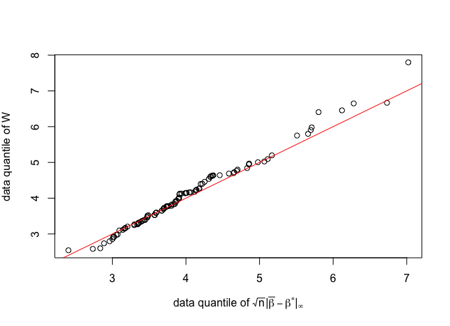
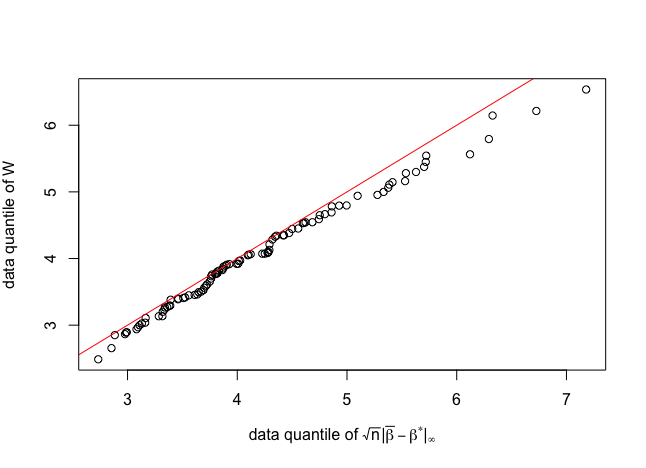
In this section, we evaluate the performance of the proposed bootstrap-assist procedure in simultaneous inference. We consider the model (2.2), where ’s are i.i.d. Student’s -distributions with or . Let . We pick and in the numerical setup. For the true transition matrix , we consider the following designs.
-
(1)
Banded: and .
-
(2)
Block diagonal: , where each has on the diagonal and on the superdiagonal with
The design in (1) is further scaled by to ensure that . Hence sparse symmetric matrices are generated in (1) and sparse asymmetric matrices are constructed in (2). We draw the qq-plots of the data quantile of versus the data quantile of defined in Theorem 2.12 from duplicates. The qq-plots are shown in figure 2 and figure 2 for banded and block diagonal designs respectively.
Appendix A Proofs of Results in Section 2
Before proceeding with the proofs, we state a helpful lemma that is repeatedly used throughout the paper and present its proof. This simply lemma is an application of the triangle inequality to the product of two matrices.
Lemma A.1.
Let and be symmetric matrices and . Suppose and . Then .
Proof of Lemma A.1.
Since and , . Hence, by triangular inequality,
∎
Proof of Theorem 2.5.
Proof of Theorem 2.7.
The next Lemma provides a high probability bound on , which will be used in the proof of Theorem 2.8.
Lemma A.2.
Suppose that for all . Then it holds that
for some constant .
Proof of Lemma A.2.
Proof of Theorem 2.8.
By Taylor expansion, we write
where the remainder
where for some lying between and . Now we analyze the above terms respectively. First we see that by assumption (A1). To analyze , denote . Then we write
Thus, by theorem 3.6 and theorem 2.7, with probability tending to 1,
by assumption (A3). Finally, by Lemma A.2 and Theorem 2.7, with probability tending to 1, it holds that
Therefore,
where
∎
Proof of Theorem 2.9.
The proof of Theorem 4.1 can be easily generalized to dimensional space, thus it still holds for . By Theorem 4.1, we have for any ,
| (A.3) |
where
| (A.4) |
Now choose in (A) for some constant . For sufficiently large , basic algebra shows that
| (A.5) |
since the order of dominates the order of . Moreover,
| (A.6) |
by a proper choice of constant . Also, by assumption (A5), and
Thus the proof is completed. ∎
Proof of Theorem 2.11.
First, we collect several useful results.
-
(i)
With probability at least , and by Theorem 2.5. Therefore, and by assumption (A2).
-
(ii)
With probability at least , Lemma 3.7 and the order comes from assumptions (A1) and (A2).
-
(iii)
Similar to the proof of Lemma 3.7, we have with probability at least ,
-
(iv)
Similar to the proof of Lemma 3.5, we have with probability at least ,
Proof of Theorem 2.12.
By theorem 2.8, we see that
where and . Define with and
Let , where the sequence is defined in theorem 2.9. From the proof of Lemma 3.2 in Chernozhukov et al., (2013), we have
| (A.7) | ||||
| (A.8) |
Therefore, by theorem 2.9, (A.7) and (A.8), we have for every ,
Furthermore, following the same spirit as the proof of Theorem 3.2 in Chernozhukov et al., (2013), we see that
Now that and from Theorem 2.8, we only need to choose , such that and . Let . Then we see that the conditions that and are satisfied by Theorem 2.11 and the scaling hypothesis. ∎
Appendix B Proofs of Results in Section 3
Proof of Lemma 3.1.
Define the filtration with , and let be a projection. Conventionally it follows that for . We can write
where . By the Markov inequality, for , we have
| (B.1) |
for some to be determined later. We shall bound the right-hand side of (B) with a suitable choice of . Observing that is a sequence of martingale differences with respect to , we then seek an upper bound on . It follows that
| (B.2) |
where is an i.i.d. copy of and
Denote . Note that is a positive integer. For , we have
For , we also have
Basic algebra shows that
| (B.3) |
where (1) comes from the independence of and . To analyze (B), we further compute
| (B.4) |
Plugging (B) into (B) yields, for some constant , that
| (B.5) |
where (1) uses the inequality that for and (2) uses Stirling formula and the fact that . Let and . Then we obtain
| (B.6) |
Furthermore,
| (B.7) |
Take and by (B) we have
| (B.8) |
Similarly, for , since ,
By the same argument, we immediate have
| (B.9) |
where and . By (B.8), (B.9) and symmetrization argument, we complete the proof. ∎
Proof of Corollary 3.3.
It follows from the proof of lemma 3.1 without any extra technical difficulty. ∎
Proof of Theorem 3.5.
Define be defined as for , and hence . Let . Observe that
By lemma 3.1, take
A union bound yields
where . ∎
Proof of Theorem 3.6.
Proof of Lemma 3.7.
The strategy is to consider each component of and take a union bound. Observe that
Since is bounded, by the mean value theorem, we have that for some between and ,
So it can be verified that satisfies the conditions in Corollary 2.5 of Liu and Zhang, (2021). By Corollary 2.5 of Liu and Zhang, (2021), it holds that
with probability at least for some positive constant . Moreover,
where the last inequality comes from the fact that has bounded second moment. ∎
Appendix C Proofs of Result in Section 4
Before proving Theorem 4.1, we will first state and prove the corresponding lemmas in the outline listed at the end of section 4.
Lemma C.1.
Suppose for all and the odd function satisfies that and , then we have
for some constants .
Proof of Lemma C.1.
Let . For any , by Markov inequality we have
| (C.1) |
Notice that the martingale difference satisfies
Thus,
By Burkholder inequality (Burkholder, (1973)), we have
| (C.2) |
Hence, by (C.1),
Finally, symmetrization and a union bound give the desired result. ∎
Lemma C.2.
Under the assumptions in Lemma C.1, it holds that
Proof of Lemma C.2.
By the property of and the mean value theorem, we have . Consider the first coordinate of . We can write , where . Observe that is a martingale difference adapted to the filtration and that . We shall establish a Bernstein-type inequality for the sum of martingale differences :
| (C.3) |
We now bound from above. By the tower property,
| (C.4) |
Now, consider
| (C.5) |
where the inequality (1) makes use of the fact that . Plug (C) into (C) and we obtain
| (C.6) |
Iterating this procedure yields
| (C.7) |
Choose and by (C.3) we have
The symmetrization argument and a union bound deliver the desired result. ∎
Lemma C.3.
Suppose the scaling condition holds that . Assume that for all . Then we have the following Gaussian Approximation result that
for some constants .
Proof of Lemma C.3.
Recall that , thus
Observe that are independent random variables. We shall apply Corollary 2.1 of Chernozhukov et al., (2013) by verifying the condition (E.1) therein. For completeness, the conditions are stated below.
-
(i)
for all .
-
(ii)
for some and all .
-
(iii)
.
To verify condition (i), we see that
where is the -th row of and is the -th diagonal entry of . Now we check condition (ii). By Theorem 3.2 of Burkholder, (1973), we have for ,
Therefore, take for sufficiently large and we have
Moreover, for a suitable choice of ,
Hence, condition (ii) is satisfied. Condition (iii) is guaranteed by the scaling assumption. ∎
Now, we are ready to give the proof of Theorem 4.1.
Proof of Theorem 4.1.
References
- Basu and Michailidis, (2015) Basu, S. and Michailidis, G. (2015). Regularized estimation in sparse high-dimensional time series models. The Annals of Statistics, 43(4):1535–1567.
- Bernstein, (1946) Bernstein, S. (1946). The theory of probabilities.
- Bickel, (1975) Bickel, P. J. (1975). One-step huber estimates in the linear model. Journal of the American Statistical Association, 70(350):428–434.
- Bühlmann and Van De Geer, (2011) Bühlmann, P. and Van De Geer, S. (2011). Statistics for high-dimensional data: methods, theory and applications. Springer Science & Business Media.
- Burkholder, (1973) Burkholder, D. L. (1973). Distribution function inequalities for martingales. the Annals of Probability, pages 19–42.
- Cai et al., (2011) Cai, T., Liu, W., and Luo, X. (2011). A constrained minimization approach to sparse precision matrix estimation. Journal of the American Statistical Association, 106(494):594–607.
- Candes and Tao, (2007) Candes, E. and Tao, T. (2007). The dantzig selector: Statistical estimation when p is much larger than n. The annals of Statistics, 35(6):2313–2351.
- Chernozhukov et al., (2015) Chernozhukov, V., Chetverikov, D., and Kato, K. (2015). Comparison and anti-concentration bounds for maxima of gaussian random vectors. Probability Theory and Related Fields, 162(1):47–70.
- Chernozhukov et al., (2013) Chernozhukov, V., Chetverikov, D., Kato, K., et al. (2013). Gaussian approximations and multiplier bootstrap for maxima of sums of high-dimensional random vectors. The Annals of Statistics, 41(6):2786–2819.
- Fan et al., (2017) Fan, J., Li, Q., and Wang, Y. (2017). Estimation of high dimensional mean regression in the absence of symmetry and light tail assumptions. Journal of the Royal Statistical Society. Series B, Statistical methodology, 79(1):247.
- Friedman et al., (2008) Friedman, J., Hastie, T., and Tibshirani, R. (2008). Sparse inverse covariance estimation with the graphical lasso. Biostatistics, 9(3):432–441.
- Han et al., (2015) Han, F., Lu, H., and Liu, H. (2015). A direct estimation of high dimensional stationary vector autoregressions. Journal of Machine Learning Research.
- Hsu et al., (2008) Hsu, N.-J., Hung, H.-L., and Chang, Y.-M. (2008). Subset selection for vector autoregressive processes using lasso. Computational Statistics & Data Analysis, 52(7):3645–3657.
- Javanmard and Montanari, (2014) Javanmard, A. and Montanari, A. (2014). Confidence intervals and hypothesis testing for high-dimensional regression. The Journal of Machine Learning Research, 15(1):2869–2909.
- Juselius, (2006) Juselius, K. (2006). The cointegrated VAR model: methodology and applications. Oxford university press.
- Li and Zhu, (2008) Li, Y. and Zhu, J. (2008). L 1-norm quantile regression. Journal of Computational and Graphical Statistics, 17(1):163–185.
- Liu and Zhang, (2021) Liu, L. and Zhang, D. (2021). Robust estimation of high-dimensional vector autoregressive models. arXiv preprint arXiv:2109.10354.
- Loh, (2017) Loh, P.-L. (2017). Statistical consistency and asymptotic normality for high-dimensional robust -estimators. The Annals of Statistics, 45(2):866–896.
- Loh, (2018) Loh, P.-L. (2018). Scale calibration for high-dimensional robust regression. arXiv preprint arXiv:1811.02096.
- Loh and Wainwright, (2012) Loh, P.-L. and Wainwright, M. J. (2012). High-dimensional regression with noisy and missing data: Provable guarantees with nonconvexity. The Annals of Statistics, pages 1637–1664.
- Loh and Wainwright, (2017) Loh, P.-L. and Wainwright, M. J. (2017). Support recovery without incoherence: A case for nonconvex regularization. The Annals of Statistics, 45(6):2455–2482.
- Massart, (2007) Massart, P. (2007). Concentration inequalities and model selection, volume 6. Springer.
- Meinshausen and Bühlmann, (2006) Meinshausen, N. and Bühlmann, P. (2006). High-dimensional graphs and variable selection with the lasso. The annals of statistics, 34(3):1436–1462.
- Merlevède et al., (2009) Merlevède, F., Peligrad, M., Rio, E., et al. (2009). Bernstein inequality and moderate deviations under strong mixing conditions. In High dimensional probability V: the Luminy volume, pages 273–292. Institute of Mathematical Statistics.
- Nardi and Rinaldo, (2011) Nardi, Y. and Rinaldo, A. (2011). Autoregressive process modeling via the lasso procedure. Journal of Multivariate Analysis, 102(3):528–549.
- Negahban and Wainwright, (2011) Negahban, S. and Wainwright, M. J. (2011). Estimation of (near) low-rank matrices with noise and high-dimensional scaling. The Annals of Statistics, pages 1069–1097.
- Negahban et al., (2012) Negahban, S. N., Ravikumar, P., Wainwright, M. J., and Yu, B. (2012). A unified framework for high-dimensional analysis of -estimators with decomposable regularizers. Statistical science, 27(4):538–557.
- Pan et al., (2021) Pan, X., Sun, Q., and Zhou, W.-X. (2021). Iteratively reweighted 1-penalized robust regression. Electronic Journal of Statistics, 15(1):3287–3348.
- Shan, (2005) Shan, J. (2005). Does financial development ’lead’ economic growth? a vector auto-regression appraisal. Applied Economics, 37(12):1353–1367.
- Tibshirani, (1996) Tibshirani, R. (1996). Regression shrinkage and selection via the lasso. Journal of the Royal Statistical Society: Series B (Methodological), 58(1):267–288.
- Van de Geer et al., (2014) Van de Geer, S., Bühlmann, P., Ritov, Y., and Dezeure, R. (2014). On asymptotically optimal confidence regions and tests for high-dimensional models. The Annals of Statistics, 42(3):1166–1202.
- Wainwright, (2019) Wainwright, M. J. (2019). High-dimensional statistics: A non-asymptotic viewpoint, volume 48. Cambridge University Press.
- Wu, (2005) Wu, W. B. (2005). Nonlinear system theory: Another look at dependence. Proceedings of the National Academy of Sciences, 102(40):14150–14154.
- Wu and Liu, (2009) Wu, Y. and Liu, Y. (2009). Variable selection in quantile regression. Statistica Sinica, pages 801–817.
- Wu and Zhou, (2010) Wu, Y. and Zhou, X. (2010). Var models: Estimation, inferences, and applications. In Handbook of Quantitative Finance and Risk Management, pages 1391–1398. Springer.
- Yuan and Lin, (2007) Yuan, M. and Lin, Y. (2007). Model selection and estimation in the gaussian graphical model. Biometrika, 94(1):19–35.
- Zhang and Zhang, (2014) Zhang, C.-H. and Zhang, S. S. (2014). Confidence intervals for low dimensional parameters in high dimensional linear models. Journal of the Royal Statistical Society: Series B (Statistical Methodology), 76(1):217–242.
- Zhang, (2019) Zhang, D. (2019). Robust estimation of the mean and covariance matrix for high dimensional time series. Statistica Sinica, to appear.
- Zhang and Wu, (2017) Zhang, D. and Wu, W. B. (2017). Gaussian approximation for high dimensional time series. The Annals of Statistics, 45(5):1895–1919.
- Zhang and Cheng, (2017) Zhang, X. and Cheng, G. (2017). Simultaneous inference for high-dimensional linear models. Journal of the American Statistical Association, 112(518):757–768.
- Zou, (2006) Zou, H. (2006). The adaptive lasso and its oracle properties. Journal of the American statistical association, 101(476):1418–1429.