High-dimensional single-index models:
link estimation and marginal inference
Abstract.
This study proposes a novel method for estimation and hypothesis testing in high-dimensional single-index models. We address a common scenario where the sample size and the dimension of regression coefficients are large and comparable. Unlike traditional approaches, which often overlook the estimation of the unknown link function, we introduce a new method for link function estimation. Leveraging the information from the estimated link function, we propose more efficient estimators that are better aligned with the underlying model. Furthermore, we rigorously establish the asymptotic normality of each coordinate of the estimator. This provides a valid construction of confidence intervals and -values for any finite collection of coordinates. Numerical experiments validate our theoretical results.
1. Introduction
We consider i.i.d. observations with a -dimensional Gaussian feature vector , and each scalar response belongs to a set (e.g., ), following the single-index model:
| (1) |
where is an unknown deterministic coefficient vector, and is an unknown deterministic function, referred to as the link function, with being the index. To identify the scale of , we assume . The model includes common scenarios such as:
-
•
Linear regression: with by setting .
-
•
Poisson regression: by setting .
-
•
Binary choice models: with . This includes logistic regression for and the probit model by setting as the cumulative distribution function of the standard Gaussian distribution.
We are interested in a high-dimensional setting, where both the sample size and the coefficient dimension are large and comparable. Specifically, this study examines the proportionally high-dimensional regime defined by:
| (2) |
where is a positive constant.
The single-index model (1) possesses several practically important properties. First, it mitigates concerns about model misspecification, as it eliminates the need to specify . Second, this model bypasses the curse of dimensionality associated with function estimation since the input index is a scalar. This advantage is particularly notable in comparison with nonparametric regression models, such as , where remains unspecified. Third, the model facilitates the analysis of the contribution of each covariate, for , to the response by testing against . Owing to these advantages, single-index models have been actively researched for decades (Powell et al., 1989; Härdle and Stoker, 1989; Li and Duan, 1989; Ichimura, 1993; Klein and Spady, 1993; Hristache et al., 2001; Nishiyama and Robinson, 2005; Dalalyan et al., 2008; Alquier and Biau, 2013; Eftekhari et al., 2021; Bietti et al., 2022; Fan et al., 2023), attracting interest across a broad spectrum of fields, particularly in econometrics (Horowitz, 2009; Li and Racine, 2023).
In the proportionally high-dimensional regime as defined in (2), the single-index model and its variants have been extensively studied. For logistic regression, which is a particular instance of the single-index model, Sur et al. (2019); Salehi et al. (2019) have investigated the estimation and classification errors of the regression coefficient estimators . Furthermore, Sur and Candès (2019); Zhao et al. (2022); Yadlowsky et al. (2021) have developed methods for asymptotically valid statistical inference. In the case of generalized linear models with a known link function , Rangan (2011); Barbier et al. (2019) have characterized the asymptotic behavior of the coefficient estimator, while Sawaya et al. (2023) have derived the coordinate-wise marginal asymptotic normality of an adjusted estimator of . For the single-index model with an unknown link function , the seminal work by Bellec (2022) establishes the (non-marginal) asymptotic normality of estimators, even when there is link misspecification. However, the construction of an estimator for the link function and the marginal asymptotic normality of the coefficient estimator are issues that have not yet been fully resolved.
Inspired by these seminal works, the following questions naturally arise:
-
(i)
Can we consistently estimate the unknown link function ?
-
(ii)
Can we rigorously establish marginal statistical inference for each coordinate of ?
-
(iii)
Can we improve the estimation efficiency by utilizing the estimated link function?
This paper aims to provide affirmative answers to these questions. Specifically, we propose a novel estimation methodology comprising three steps. First, we construct an estimator for the index , based on the distributional characteristics of a pilot estimator for . Second, we develop an estimator for the link function by utilizing the estimated index in a nonparametric regression problem that involves errors-in-variables. Third, we design a new convex loss function that leverages the estimated link function to estimate . To conduct statistical inference, we investigate the estimation problem of inferential parameters necessary for establishing coordinate-wise asymptotic normality in high-dimensional settings.
Our contributions are summarized as follows:
-
-
Link estimation: We propose a consistent estimator for the link function , which is of practical significance as well as estimating coefficients. This aids in interpreting the model via the link function and mitigates negative impacts on coefficient estimation due to link misspecification.
-
-
Marginal inference: We establish the asymptotic normality for any finite subset of the coordinates of our estimator, facilitating coordinate-wise inference of . This approach allows us not only to test each variable’s contribution to the response but also to conduct variable selection based on importance statistics for each feature.
-
-
Efficiency improvement: By utilizing the consistently estimated link function, we anticipate that our estimator of will be more efficient than previous estimators that rely on potentially misspecified link functions. We predominantly validate this efficiency through numerical simulations.
From a technical perspective, we leverage the proof strategy in Zhao et al. (2022) to demonstrate the marginal asymptotic normality of our estimator for . Specifically, we extend the arguments to a broader class of unregularized M-estimators, whereas Zhao et al. (2022) originally considered the maximum likelihood estimator (MLE) for logistic regression.
1.1. Marginal Inference in High Dimensions
We review key technical aspects of statistical inference for each coordinate in the proportionally high-dimensional regime (2). We maintain of constant order by considering the setting . We define as the precision matrix for the distribution of and set . An unbiased estimator of can be constructed using nodewise regression (cf. Section 5.1 in Zhao et al. (2022)). For simplicity, we assume is known, following prior studies.
In the high-dimensional regime (2), statistical inference must address two components: the asymptotic distribution and the inferential parameters of an estimator. We review the asymptotic distribution of the MLE for logistic regression. According to Zhao et al. (2022), for all such that as , the estimator achieves the following asymptotic normality:
| (3) |
Here, we define and as the asymptotic bias and variance, respectively, ensuring the convergence (3). It is crucial to note that both the estimator and the target scale as here.
To perform statistical inference based on (3), it is necessary to estimate the inferential parameters and . Several studies including El Karoui et al. (2013); Thrampoulidis et al. (2018); Sur and Candès (2019); Loureiro et al. (2021) theoretically characterize these parameters as solutions to a system of nonlinear equations that depend on the data-generating process and the loss function. Additionally, various approaches have been developed to practically solve the equations by determining their hyperparameter under different conditions. Specifically, Sur and Candès (2019) introduces ProbeFrontier for estimating based on the asymptotic existence/non-existence boundary of the maximum likelihood estimator (MLE) in logistic regression. SLOE, proposed by Yadlowsky et al. (2021), enhances this estimation using a leave-one-out technique. Moreover, Sawaya et al. (2023) takes a different approach to estimate for generalized linear models.
For single-index models, Bellec (2022) introduces observable adjustments that estimate the inferential parameters directly under the identification condition irrespective of link misspecification, bypassing the system of equations. In our study, we develop an estimator for the single-index model satisfying the asymptotic normality (3), with corresponding estimators for the inferential parameters using observable adjustments.
1.2. Related Works
Research into the asymptotic behavior of statistical models in high-dimensional settings, where both and diverge proportionally, has gained momentum in recent years. Notable areas of exploration include (regularized) linear regression models (Donoho et al., 2009; Bayati and Montanari, 2011b; Krzakala et al., 2012; Bayati et al., 2013; Thrampoulidis et al., 2018; Mousavi et al., 2018; Takahashi and Kabashima, 2018; Miolane and Montanari, 2021; Guo and Cheng, 2022; Hastie et al., 2022; Li and Sur, 2023), robust estimation (El Karoui et al., 2013; Donoho and Montanari, 2016), generalized linear models (Rangan, 2011; Sur et al., 2019; Sur and Candès, 2019; Salehi et al., 2019; Barbier et al., 2019; Zhao et al., 2022; Tan and Bellec, 2023; Sawaya et al., 2023), low-rank matrix estimation (Deshpande et al., 2017; Macris et al., 2020; Montanari and Venkataramanan, 2021), and various other models (Montanari et al., 2019; Loureiro et al., 2021; Yang and Hu, 2021; Mei and Montanari, 2022). These investigations focus primarily on the convergence limits of estimation and prediction errors. Theoretical analyses have shown that classical statistical estimation often fails to accurately estimate standard errors and may lack key desirable properties such as asymptotic unbiasedness and asymptotic normality.
In such analyses, the following theoretical tools have been employed: (i) the replica method (Mézard et al., 1987; Charbonneau et al., 2023), (ii) approximate message passing algorithms (Donoho et al., 2009; Bolthausen, 2014; Bayati and Montanari, 2011a; Feng et al., 2022), (iii) the leave-one-out technique (El Karoui et al., 2013; El Karoui, 2018), (iv) the convex Gaussian min-max theorem (Thrampoulidis et al., 2018), (v) second-order Poincaré inequalities (Chatterjee, 2009; Lei et al., 2018), and (vi) second-order Stein’s formulae (Bellec and Zhang, 2021; Bellec and Shen, 2022). Although these tools were initially proposed for analyzing linear models with Gaussian design, they have been extensively adapted to a diverse range of models. In this study, we apply observable adjustments based on second-order Stein’s formulae (Bellec, 2022) to directly estimate the asymptotic bias and variance of coefficient estimators. Furthermore, we provide a comprehensive proof of marginal asymptotic normality, extending the work of Zhao et al. (2022) to a wider array of estimators.
1.3. Notation
Define for . For a vector , we write . For a collection of indices , we define a sub-vector as a slice of . For a matrix , we define its minimum and maximum eigenvalues by and , respectively. For a function , we say the derivative of and the th-order derivative. For a function and a vector , denotes a vector by elementwise operations.
1.4. Organization
We organize the remainder of the paper as follows: Section 2 presents our estimation procedure. Section 3 describes the asymptotic properties of the proposed estimator and develops a statistical inference method. Section 4 provides several experiments to validate our estimation theory. Section 5 outlines the proofs of our theoretical results. Section 6 discusses alternative designs for estimators. Finally, Section 7 concludes with a discussion of our findings. The Appendix contains additional discussions and the complete proofs.
2. Statistical Estimation Procedure
In this section, we introduce a novel statistical estimation method for single-index models as defined in (1). Our estimator is constructed through the following steps:
-
(i)
Construct an index estimator for using the ridge regression estimator , referred to as a pilot estimator. This estimator is reasonable regardless of the misspecification of the link function.
-
(ii)
Develop a function estimator for the link function , based on the distributional characteristics of the index estimator .
-
(iii)
Construct our estimator for the coefficients , using the estimated link function.
Furthermore, statistical inference additionally involves a fourth step:
-
(iv)
Estimate the inferential parameters and , conditional on the estimated link function .
In our estimation procedure, we divide the dataset into two disjoint subsets and , where are index sets such that and . Additionally, for , let and denote the design matrix and response vector of subset , respectively. We utilize the first subset to estimate the link function (Steps (i) and (ii)), and the second subset to estimate the regression coefficients (Step (iii)) and inference parameters (Step (iv)). From a theoretical perspective, this division helps to manage the complicated dependency structure caused by data reuse. Nonetheless, for practical applications, we recommend employing all observations in each step to maximize the utilization of the data’s inherent signal strength. Here, and are the sample sizes for each partition, satisfying . We define and .
2.1. Index Estimation
In this step, we use the first subset . We define the pilot estimator as the ridge estimator, where is the regularization parameter. Further, we consider inferential parameters of , which satisfy for such that . Using these parameters, we develop an estimator for the index as follows:
| (4) |
for each . Here, and are estimators of and , defined as
| (5) |
where and . These estimators are obtained by the observable adjustment technique described in Bellec (2022).
This index estimator is approximately unbiased for the index , yielding the following asymptotic result:
| (6) |
We will provide its rigorous statement in Proposition 1 in Section 5.1.
There are other options for the pilot estimator besides the ridge estimator . If holds, the least squares estimator can be an alternative. If is a binary or non-negative integer, the MLE of logistic or Poisson regression can be a natural candidate, respectively, although the ridge estimator is valid regardless of the form that takes. In each case, the estimated inferential parameters should be updated accordingly. Details are presented in Section 6.
2.2. Link Estimation
We develop an estimator of the link function using in (4). If we could observe the true index with the unknown coefficient , it would be possible to estimate by applying standard nonparametric methods to the pairs of responses and true indices . However, as the true index is unobservable, we must estimate using given pairs of responses and contaminated indices , where . The type of error involving the regressor leads to an attenuation bias in the estimation of , known as the errors-in-variables problem. To address this issue, we utilize a deconvolution technique (Stefanski and Carroll, 1990) to remove the bias stemming from error-in-variables asymptotically. Further details of the deconvolution are provided in Section C.
We define an estimator of . In preparation, we specify a kernel function , and define a deconvolution kernel as follows:
| (7) |
where is a bandwidth, is an imaginary unit, is a ratio of the inferential parameters, and and are the Fourier transform of and the density function of , respectively. We then define our estimator of as
| (8) |
where is a monotonization operator, specified later, which maps any measurable function to a monotonic function, and is a Nadaraya-Watson estimator obtained by the deconvolution kernel. We will prove the consistency of this estimator in Theorem 1 in Section 3.
The monotonization operation on is justifiable because the true link function is assumed to be monotonic. One simple choice for , applicable to any measurable function , is
| (9) |
This definition holds for all . Another effective alternative is the rearrangement operator (Chernozhukov et al., 2009). This operator monotonizes a measurable function within a compact interval :
| (10) |
This operator, which sorts the values of in increasing order, is robust against local fluctuations such as function bumps. Thus, it effectively addresses bumps in arising from kernel-based methods.
2.3. Coefficient Estimation
We next propose our estimator of using obtained in (8). In this step, we consider the link estimator from as given, and estimate using . To facilitate this, we introduce the surrogate loss function for , with , , and any measurable function :
| (11) |
where is a function such that . This function can be viewed as a natural extension of the matching loss (Auer et al., 1995) used in generalized linear models. If is strictly increasing, then the loss is strictly convex in . Moreover, the surrogate loss is justified by the characteristics of the true parameter as follows (Agarwal et al., 2014):
| (12) |
provided that is integrable. The surrogate loss aligns with the negative log-likelihood when is known and serves as a canonical link function, thereby making the surrogate loss minimizer a generalization of the MLEs in generalized linear models.
Using the second dataset with any given function , we define our estimator of as
| (13) |
where is a convex regularization function. Finally, we substitute the link estimator into (13) to obtain our estimator . The use of a nonzero regularization term, , is beneficial in cases where the minimizer (13) is not unique or does not exist; see, for example, Candès and Sur (2020) for the logistic regression case.
2.4. Inferential Parameter Estimation
We finally study estimators for the inferential parameters of our estimator , which are essential for statistical inference as discussed in Section 1.1. As established in (3), it is necessary to estimate the asymptotic bias and variance that satisfy the following relationship:
| (14) |
conditional on and consequently on .
We develop estimators for these inferential parameters using observable adjustments as suggested by Bellec (2022), in accordance with the estimator (13). For any measurable function , we define and for . When incorporating into (13) with , we propose the following estimators:
| (15) |
In the case where holds, we define
| (16) |
A theoretical justification for the asymptotic normality with these estimators and their application in inference is provided in Section 3.3.
3. Main Theoretical Results of Proposed Estimators
This section presents theoretical results for our estimation framework. Specifically, we prove the consistency of the estimator for the link function , and the asymptotic normality of the estimator for the coefficient vector . Outlines of the proofs for each assertion will be provided in Section 5.
3.1. Assumptions
As a preparation, we present some assumptions.
Assumption 1 (Data-splitting in high dimensions).
There exist constants with independent of such that holds.
Assumption 1 requires that the split subsamples, as described at the beginning of Section 2, have the same order of sample size.
Assumption 2 (Gaussian covariates and identification).
Each row of the matrix independently follows with obeying and with a constant .
It is common to assume Gaussianity of covariates in the proportionally high-dimensional regime, as mentioned in Section 1.2. The condition is necessary to identify the scale of , which ensures the uniqueness of the estimator in the single-index model with an unknown link function . For example, without this condition, it would be impossible to distinguish between and , where , for any . Furthermore, the assumption of upper and lower bounds on the eigenvalues of implies that .
Assumption 3 (Monotone and smooth link function).
There exists a constant such that holds for any . Also, there exist constants and such that , exists for , and holds for every for some .
Assumption 3 restricts the class of link functions to those that are monotonic. This class has been extensively reviewed in the literature, with Balabdaoui et al. (2019) providing a comprehensive discussion. It encompasses a wide range of applications, including utility functions, growth curves, and dose-response models (Matzkin, 1991; Wan et al., 2017; Foster et al., 2013). Furthermore, under a monotonically increasing link function, the sign of is identified, so that we can identify only by the scale condition .
Assumption 4 (Moment conditions of ).
holds. Further, is continuous in for defined in Assumption 3.
The continuity of is maintained in many commonly used models, particularly when is continuous. For instance, the Poisson regression model defines , and binary choice models specify .
3.2. Consistency of Link Estimation
We demonstrate the uniform consistency of the link estimator in (8) over closed intervals. We consider the -order kernel that satisfies
| (17) |
for . We then obtain the following:
Theorem 1.
Here, according to Fan and Truong (1993), the logarithmic rate reaches a lower bound, indicating that this rate cannot be improved.
3.3. Marginal Asymptotic Normality of Coefficient Estimators
This section demonstrates the marginal asymptotic normality of our estimator for , facilitated by the estimators of the inferential parameters, and . These results are directly applicable to hypothesis testing and the construction of confidence intervals for any finite subset of the ’s.
3.3.1. Unit Covariance () and Case
As previously noted, the inferential parameters vary depending on the estimator considered. In this section, we focus on the ridge regularized estimator with unit covariance . We will also present additional results for generalized covariance matrices and the ridgeless scenario later.
Theorem 2.
We consider the coefficient estimator with , and the inferential estimators , associated with the link estimator . Suppose that and Assumptions 1-3 hold. Then, a conditional distribution of with a fixed event on satisfies the following: for any coordinate satisfying , we have
| (19) |
as with the regime (2). Moreover, for any finite set of coordinates satisfying , we have, as ,
| (20) |
This result also implies that is an asymptotically unbiased estimator of . Note that the convergence of the conditional distribution is ensured by the non-degeneracy property of the conditional event, as defined by ; see Goggin (1994) for details.
We highlight two key contributions of Theorem 2. First, it remains valid even when the ratio exceeds one, a notable distinction compared to a similar result by Bellec (2022), which holds only when is less than one. Second, the statistic is independent of any unknown parameters, contrasting with, for example, the marginal asymptotic normality in logistic regression by Zhao et al. (2022), which relies on unknown inferential parameters.
Application to Statistical Inference: From Theorem 2, we construct a confidence interval for each with a confidence level as follows:
| (21) |
where and is the -quantile of the standard normal distribution. This construction ensures the coverage probability adheres to the specified confidence level asymptotically.
Corollary 1.
Hence, for testing the hypothesis against at level , we can use the corrected -statistics in (19). The test that rejects the null hypothesis if
| (23) |
controls the asymptotic size of the test at the level . Additionally, it is feasible to develop a variable selection procedure that identifies variables related to the response. Specifically, the -value associated with and the statistic can serve as importance statistics for the th covariate. This approach facilitates variable selection procedures that control the false discovery rate, as detailed in sources such as Benjamini and Hochberg (1995); Candes et al. (2018); Xing et al. (2023); Dai et al. (2023).
3.3.2. General Covariance and Case
We extend Theorem 2 to scenarios with a general covariance matrix in unregularized settings. To this end, we utilize the estimators , which are defined for inferential parameters in Section 2.4. Recall that the precision matrix is defined as .
Theorem 3.
We consider the coefficient estimator with , and the inferential estimators , associated with the link estimator . Suppose that Assumptions 1-3 hold. Then, a conditional distribution of with a fixed event on satisfies the following: for any coordinate satisfying , we have
| (24) |
as with the regime (2). Moreover, for a finite set of coordinates , we have
| (25) |
where the submatrix consists of for .
4. Experiments
This section provides numerical validations of our estimation framework as outlined in Section 2. The efficiency of our proposed estimator is subsequently compared with that of other estimators.
We examine two high-dimensional scenarios: and . For the scenario where , we assume the true coefficient vector follows a uniform distribution on the sphere: . In the case of , we set and . We generate response variables for Gaussian predictors with an identity covariance matrix , under the following four scenarios:
-
(i)
Cloglog: with ;
-
(ii)
xSqrt: with ;
-
(iii)
Cubic: cubic regression with and ;
-
(iv)
Piecewise: piecewise regression with and .
4.1. Index Estimator
We validate the normal approximation of the index estimator as shown in (6). For cases where , we set for the Cloglog model and for the other models. For cases where , we set and apply the ridge regularized estimator to all models. We assign the maximum likelihood estimator (MLE) of logistic regression to the pilot estimator for (i) Cloglog, the MLE of Poisson regression for (ii) xSqrt, and the least squares estimator for both (iii) Cubic and (iv) Piecewise models. We calculate using replications for each setup.
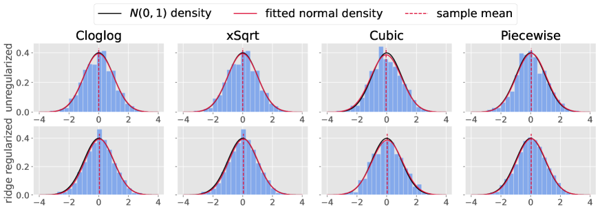
Figure 1 displays the results. In all settings, the difference between the index estimator and the index follows a Gaussian distribution, as expected.
4.2. Link Function Estimator
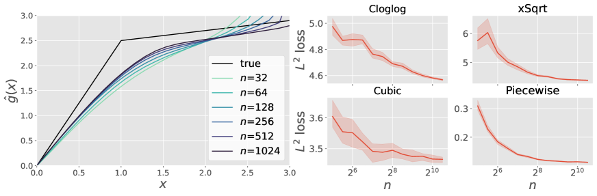
Next, we evaluate the numerical performance of the link estimator , constructed from , using a fixed bandwidth for each . Figure 2 (left panel) shows that the estimation error of for (iv) Piecewise uniformly approaches zero as the sample size increases. The right four panels in Figure 2 display the squared losses of evaluated over the interval , which all decrease as increases.
4.3. Our Coefficient Estimator
We examine the asymptotic normality of each coordinate of the estimator for the true coefficients. As in Section 4.2, we construct the estimator using a fixed bandwidth and apply the rearrangement operator as defined in (10) over the interval to obtain . We then compute according to (13) using when and when . Figure 3 shows the marginal normal approximation of the estimators under these conditions. All histograms closely resemble the standard normal density, corroborating the asymptotic normality stated in Theorems 2 and 3.
4.4. Efficiency Comparison
Finally, we compare the estimation efficiency of the proposed estimator with several pilot estimators. We use the effective asymptotic variance as an efficiency measure, which is the inverse of the effective signal-to-noise ratio as described in Feng et al. (2022). We estimate this variance using the statistic for an estimator . This statistic is a reasonable approximation of the asymptotic variance of the debiased version of and converges almost surely to the effective asymptotic variance under certain conditions (see Section 5 for details).
From a practical perspective, we analyze the scatter plot of and manually specify a functional form for to conduct parametric regression. We estimate parameters in different forms: for case (i), for case (ii), for case (iii), and for case (iv). We then use these estimates to construct the link function. Additionally, we introduce new data-generating processes: Logit, where ; Poisson, where ; Cubic+, where , with ; and Piecewise+, where , with .
Table 1 displays the efficiency measures for our proposed estimator and others across 100 replications. We find that our proposed estimator is generally more efficient in most settings, except when the estimators are specifically tailored to the models. This highlights the broad applicability of our estimator.
| LeastSquares | LogitMLE | PoisMLE | Proposed | |
|---|---|---|---|---|
| Logit | .525.157 | – | ||
| Cloglog | – | .271.068 | ||
| Poisson | – | .630.124 | .630.124 | |
| xSqrt | – | 1.12.290 | 1.12.290 | |
| Cubic | 1.15.258 | – | – | |
| Cubic+ | – | – | 1.74.439 | |
| Piecewise | – | – | .391.157 | |
| Piecewise+ | – | – | .330.184 |
4.5. Real Data Applications
We utilize two datasets from the UCI Machine Learning Repository (Dua and Graff, 2017) to illustrate the performance of the proposed estimator. The DARWIN dataset (Cilia et al., 2018) comprises handwriting data from 174 participants, including both Alzheimer’s disease patients and healthy individuals. The second dataset (Sakar and Sakar, 2018) features 753 attributes derived from the sustained phonation of the vowel sounds of patients, both with and without Alzheimer’s disease. We employ a leave-one-out strategy for splitting each dataset. For each subset, we compute the regularized MLE of logistic regression alongside the proposed estimate derived from it. We then estimate the effective asymptotic variance, , for each estimator. The results, presented in Tables 2–3, indicate that the proposed estimator consistently provides a more accurate estimation of the true coefficient vector compared to conventional logistic regression.
| Logit | 1.870.06 | 0.460.01 | 0.300.00 |
|---|---|---|---|
| proposed | 0.610.01 | 0.250.00 | 0.180.00 |
| Logit | 2.220.03 | 0.300.00 | 0.160.00 |
|---|---|---|---|
| proposed | 0.150.00 | 0.060.00 | 0.050.00 |
5. Proof Outline
We outline the proofs for each theorem in Section 3.
5.1. Consistency of Link Estimation (Theorem 1)
We provide an overview of the proof for Theorem 1, which comprises two primary steps: (i) the asymptotic characteristics of the index estimator discussed in Section 2.1, and (ii) demonstrating the consistency of the estimator in Section 2.2, related to .
5.1.1. Error of Index Estimator
We consider the distributional approximation (6) for the index estimator , established through observable adjustments by Bellec (2022). Theorems 4.3 and 4.4 in Bellec (2022) support the following proposition:
The proposition asserts that each for is approximately equal to the sum of the biased true index , a Gaussian error, and an additive bias term. Since has the form , its approximation error is asymptotically represented by the Gaussian term as shown in Equation (6).
5.1.2. Error of Link Estimator
Next, we prove the consistency of the link estimator using the index estimator . Suppose were exactly equivalent to . In this case, we could apply the classical result of nonparametric error-in-variables regression (Fan and Truong, 1993) to demonstrate the uniform consistency of . However, this equivalence is only asymptotic as shown in (26). Therefore, we establish that the error due to this asymptotic equivalence is negligibly small in the estimation of to complete the proof.
Specifically, we take the following steps. First, we decompose the error of into two terms. In preparation, we define as a deconvolution estimator using a deconvolution kernel using the true inferential parameters as (its precise definition is given in Section C). This estimator corresponds to the estimator for the error-in-variable setup developed by Fan and Truong (1993). Then, from the effect of the monotonization operator, we obtain the following decomposition:
| (27) |
The second term in (27) is the estimation error by the deconvolution estimator , which is proven to be according to the result of Fan and Truong (1993).
On the other hand, the first term in (27) represents how our pre-monotonized estimator in (8) approximates the estimator . Rigorously, we obtain
| (28) | |||
| (29) |
where is an inequality up to some universal constant. The first term describes the error by the index estimator . We develop an upper bound on by using the result of Proposition 1. The second term represents the discrepancy between the convolution kernels and . Note that depends on the estimator of the inferential parameter, and depends on the true value of the inferential parameter . We derive its upper bound by evaluating the error of the estimators .
By integrating these results into (27), we prove that the estimation error of is .
5.2. Marginal Asymptotic Normality (Theorem 3)
This section provides a proof sketch of Theorem 3. We specifically present a general theorem that characterizes the asymptotic normality of each coordinate of the unregularized estimator in high-dimensional settings. This discussion extends the proof provided by Zhao et al. (2022) for logistic regression.
Consider the single-index model given by (1) and an arbitrary loss function . We define an M-estimator , based on the loss function , as follows:
| (30) |
With this general setup, we establish the following statement:
Theorem 4.
This theorem establishes the marginal asymptotic normality for a broad class of estimators defined by the minimization of convex loss functions. Additionally, it demonstrates that the limiting distributional behavior of is characterized by and in the high-dimensional setting (2). Intuitively, is a scaled inner product of and , and denotes the magnitude of the orthogonal component of to .
The rigorous proof in Section D.1 is conducted in the following steps:
-
(i)
Since we have , we achieve the replacements to , to , and to . From the Cholesky factorization of , we have
(33) -
(ii)
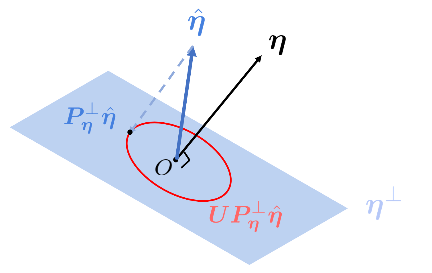
Considering the rotation around (i.e., and ), several calculations give, for ,
(34) This means that is uniformly distributed on the unit sphere in (See Figure 4).
-
(iii)
Drawing on the analogy to the asymptotic equivalence between the -dimensional standard normal distribution and , we obtain the asymptotic normality of .
6. Other Design of Pilot Estimator
We can consider alternative estimators as the pilot estimator discussed in Section 2.1. Depending on the context, choosing an appropriate pilot estimator can enhance the asymptotic efficiency of the overall estimation process. Below, we list the various estimator options and their associated values necessary for estimating their inferential parameters.
6.1. Least Squares Estimators
In the case of , we can use the least squares estimator
| (35) |
In this case, there exist corresponding inferential parameters of .
We obtain the following marginal asymptotic normality of the least-squares estimator. We recall the definition of inferential parameters in (31) and consider the corresponding parameter and by substituting . Then, we obtain the following result by a straightforward application of Theorem 4.
Corollary 2.
6.2. Maximum Likelihood Estimators
When takes discrete values, a more appropriate pilot estimator can be proposed. For binary outcomes such as in classification problems where , we can employ MLE for logistic regression:
| (38) |
In the case with , we can consider the MLE for the Poisson regression
| (39) |
Its asymptotic normality is obtained by applying Theorem 4.
Corollary 3.
In these cases, we can define values for estimating their inferential parameters. Define for logistic regression and for Poisson regression. Then, we define the values as and
| (41) |
with and . Based on this definition, we can develop a corresponding index estimator by replacing in (6) by and .
7. Conclusion and Discussion
This study establishes a novel statistical inference procedure for high-dimensional single-index models. Specifically, we develop a consistent estimation method for the link function. Furthermore, using the estimated link function, we formulate an efficient estimator and confirm its marginal asymptotic normality. This verification allows for the accurate construction of confidence intervals and -values for any finite collection of coordinates.
We identify several avenues for future research: (a) extending these results to cases where the covariate distribution is non-Gaussian, (b) generalizing our findings to multi-index models, and (c) confirming the marginal asymptotic normality of our proposed estimators under any form of regularization and covariance. These prospects offer intriguing possibilities for further exploration.
Appendix A Effect of Link Estimation on Inferential Parameters
The following theorem reveals that the estimation error of the link function is asymptotically negligible with respect to the observable adjustments.
Specifically, we consider a slightly modified version of the inferential estimator. In preparation, we define a censoring operator on a interval as . Then, for any , we define a truncation version of as , and . Further, in the case of , we define the modified estimator as
| (42) | ||||
| (43) |
Using the modified definition, we obtain the following result.
Theorem 5.
This result indicates that, since the link estimator is consistent, we can estimate the inferential parameters under the true link .
The difficulty in this proof arises from the dependence between the elements of the estimator, which cannot be handled by the triangle inequality or Hölder’s inequality, To overcome the difficulty, we utilize the Azuma-Hoeffding inequality for martingale difference sequences.
Appendix B Theoretical Efficiency Comparison
We compare the efficiency of our estimator with that of the ridge estimator as the pilot. As shown in Bellec (2022), the ridge estimator is a valid estimator for the single-index model in the high-dimensional scheme (2) even without estimating the link function .
To the aim, we define the effective asymptotic variance based on inferential parameters, which is a ratio of the asymptotic bias and the asymptotic variance. That is, our estimator has its effective asymptotic variance , and the ridge estimator has . The effective asymptotic variance corresponds to the asymptotic variance of each coordinate of the estimators with bias correction.
We give the following result for necessary and sufficient conditions for the proposed estimator to be more efficient than the least squares estimator and the ridge estimator.
Proposition 2.
This necessary and sufficient condition suggests that our estimator may have an advantage by exploiting the nonlinearity of the link function . The first reason is that, when has nonlinearity in , the residual of the proposed method is expected to be asymptotically smaller than . The second reason is that approximates the gradient mean , so this element increases when has a large gradient. Using these facsts, the proposed method incorporates the nonlinearity of and helps improve efficiency.
Proposition 3.
If , , and are fulfilled, then if and only if
| (46) |
Appendix C Nonparametric Regression with Deconvolution
In this section, we review the concept of nonparametric regression with deconvolution to address the errors-in-variable problem. To begin with, we redefine the notation only for this section. For a pair of random variables , suppose that the model is
| (47) |
and that we can only observe iid realizations of and . Here, is a random variable called measurement error or error in variables. For the identification, we assume that the distribution of is known. Let the joint distribution of be . By the definition of the conditional expectations, with
| (48) |
for the continuous random variables. The goal of the problem is to estimate the function .
If we could observe , a popular estimator of is Nadaraya-Watson estimator with
| (49) |
where is a kernel function and is the bandwidth. Since is unobservable, we alternatively construct the deconvolution estimator (Stefanski and Carroll, 1990). Let the characteristic function of , and be , and , respectively. Since the density of is the convolution of that of and , and the convolution in the frequency domain is just a multiplication, we have . Thus, the inverse Fourier transform of gives the density of . Since we know the distribution of and we can approximate by the characteristic function of the kernel density estimator of , we can construct an estimator of as
| (50) |
where we use the fact that the Fourier transform of is , which approximates . Here, is the empirical characteristic function:
| (51) |
We can rewrite (50) in a kernel form
| (52) |
with
| (53) |
Using this, Fan and Truong (1993) proposes a kernel regression estimator involving errors in variables with
| (54) |
To establish the theoretical guarantee, we impose the following assumptions:
-
(N1)
(Super-smoothness of the distribution of ) There exists constants and satisfying, as ,
(55) -
(N2)
The characteristic function of the error distribution does not vanish.
-
(N3)
Let . The marginal density of the unobserved is bounded away from zero on the interval , and has a bounded -th derivative.
-
(N4)
The true regression function has a continuous -th derivative on .
-
(N5)
The conditional second moment is continuous on , and .
-
(N6)
The kernel is a -th order kernel. Namely,
(56)
(N1) includes Gaussian distributions for and Cauchy distributions for . For a positive constant , define a set of function
| (57) |
In this setting, we have the uniform consistency of and its rate of convergence.
Lemma 1 (Theorem 2 in Fan and Truong (1993)).
Assume (N1)-(N6) and that has a bounded support on . Then, for bandwidth with ,
| (58) |
holds for any .
Furthermore, we can show the uniform convergence of the derivative of .
Lemma 2.
Under the condition of Lemma 1, we have, for any ,
| (59) |
To prove this, we use the following two lemmas.
Lemma 3.
We have, for any ,
| (60) |
and
| (61) |
Proof of Lemma 3.
We decompose the term on the left-hand side in the first statement by Euler’s formula as
| (62) | ||||
| (63) | ||||
| (64) | ||||
| (65) | ||||
| (66) |
Similarly, we obtain
| (67) | ||||
| (68) |
This completes the proof. ∎
Lemma 4.
Under the setting of Lemma 1, for bandwidth with , we have
| (69) |
Proof of Lemma 4.
At first, (N1) implies that there exists a constant such that
| (70) |
for . By the fact that and that the support of is bounded by , we have
| (71) | ||||
| (72) | ||||
| (73) | ||||
| (74) |
Here, we use the fact that . Since we choose with , we obtain the conclusion. ∎
Proof of Lemma 2.
Let . To begin with, by the triangle inequality, we have
| (75) | ||||
| (76) | ||||
| (77) | ||||
| (78) | ||||
| (79) |
where the last inequality uses the assumption . We consider showing the convergence in probability by showing the convergence. Using the triangle inequality and the Cauchy-Schwarz inequality, we have
| (80) | |||
| (81) | |||
| (82) | |||
| (83) | |||
| (84) |
Thus, to bound the right-hand side of (79), we need to show that and are bounded by constants and that , , and converge to zero.
Bound for . By triangle inequality and the fact that for , we have
| (85) |
For the first term of the left-hand side of (85), the Cauchy-Schwarz inequality gives
| (86) | ||||
| (87) |
Lemma 3 and the proof of Lemma 4 imply that this converges to zero as . Next, we consider the second term in (85). We obtain
| (88) | ||||
| (89) | ||||
| (90) | ||||
| (91) |
Thus, a classical result for the kernel density estimation gives as .
Bound for . By triangle inequality and the fact that ,
| (92) |
For the first term of the left-hand side of (92), Cauchy-Schwarz inequality gives
| (93) | ||||
| (94) |
where we use the proof of Lemma 4 for the last inequality. Lemma 3 implies that this term converges to zero as . Next, we consider the second term in (92). We have
| (95) |
Thus we have .
Bound for . By triangle inequality and the fact that for , we have
| (96) |
For the first term of the left-hand side of (96), since and ,
| (97) | ||||
| (98) |
Thus, this converges to zero in the same way as (85). For the second term in (96), by the integration by parts,
| (99) | ||||
| (100) |
Here, the second term is zero and the first term converges to uniformly.
Bound for . By triangle inequality and the fact that for , we have
| (101) |
For the first term of the left-hand side of (101), since , we have
| (102) | |||
| (103) | |||
| (104) |
Thus, this converges to zero in the same way as (92). For the second term in (101), by the integration by parts,
| (105) | ||||
| (106) |
Here, the second term is zero and the first term converges to uniformly.
Bound for and . By triangle inequality and the fact that ,
| (107) |
We have already shown , is asymptotically bounded by a constant. Similarly, we can show that is asymptotically bounded by a constant. Combining these results together, we conclude that the first term of (79) is .
Next, we consider the second term of (79). Since is asymptotically bounded uniformly on by the results above, we have only to show that . This holds since
| (108) |
This concludes that as . ∎
Appendix D Proofs of the Results
For a convex function and a constant , define the proximal operator as
| (109) |
D.1. Proof of Master Theorem
First, we define the notation used in the proof. We consider an invertible matrix that satisfies . Define, for each ,
| (110) |
Proof of Theorem 4.
We consider the following three steps.
Step 1: Reduction to standard Gaussian features. Note that the single-index model is equivalent to . Since , we have . Hence, is the estimator corresponding to the true parameter and features .
We can choose to be a Cholesky factorization so that and with by (110). This follows from the fact that since , where denotes the vector without th coordinate. Since we can generalize this to any coordinate by permutation, we obtain
| (111) |
for each and any pair .
Step 2: Reduction to uniform distribution on sphere. Define an orthogonal projection matrix onto , and an orthogonal projection matrix onto the orthogonal complement of . Let be any orthogonal matrix obeying , namely, any rotation operator about . Then, since , we have
| (112) |
Using this, we obtain
| (113) |
where the first identity follows from the fact that since is the estimator with a true coefficient and features drawn iid from , by and . (113) reveals that is rotationally invariant about , lies in , and has a unit norm. This means is uniformly distributed on the unit sphere lying in .
Step 3: Deriving asymptotic normality. The result of the previous step gives us
| (114) |
where . Triangle inequalities yield that
| (115) |
Since and , we obtain . Therefore, this fact and (114) imply that
| (116) |
where . Here we use the fact that the covariance matrix of is . Assumptions and complete the proof. ∎
D.2. Proof of Theorem 1
Let be the ratio , where and are true inferential parameters of the pilot estimator .
Proof of Proposition 1.
First, define . We also define
| (117) |
Let be the mean squared error . Since is a ridge estimator, Theorem 4.3 in Bellec (2022) implies,
| (118) |
with . Since ridge regression satisfies with a constant depending on the regularization parameter by the KKT condition, we have . Hence,
| (119) |
as for each . By using the fact that for , , and by the definition of the proximal operator, we obtain
| (120) |
as . Next, we consider to replace with observable adjustments . Theorem 4.4 in Bellec (2022) gives their consistency:
| (121) | |||
| (122) |
where we define and are positive constants. Proposition 3.1 in Bellec (2022) implies that for a constant . Also, Theorem 4.4 in Bellec (2022) implies that . By using these results, we have , , and as since the sign of is specified by an assumption. Then, triangle inequality implies
| (123) | |||
| (124) | |||
| (125) |
which converges in probability to zero. ∎
Lemma 5.
For , define with and . We also define
| (126) |
Then, under the setting of Theorem 1, we have, as ,
| (127) |
Proof of Lemma 5.
Denote We rewrite the kernel function for deconvolution in (8) as
| (128) |
and also introduce an approximated version of the kernel function as
| (129) |
The difference here is that the parameter is replaced by . We also define .
At first, we have
| (130) | ||||
| (131) | ||||
| (132) | ||||
| (133) | ||||
| (134) | ||||
| (135) | ||||
| (136) |
where , , and . Here, and converge to positive constants by the consistency of the deconvoluted kernel density estimator. We proceed to bound each term on the right-hand side. First, we bound (136). -Lipschitz continuity of with respect to yields
| (137) | |||
| (138) | |||
| (139) |
Theorem 4.4 in Bellec (2022) implies that since
| (140) |
Hence, as we choose such that for some , we obtain
| (141) |
Next, we bound (135). For any , we have
| (142) |
where the last inequality follows from 1-Lipschitz continuity of and . Since is supported on , we have
| (143) | |||
| (144) | |||
| (145) |
Here, we can use the fact that, by the triangle inequality,
| (146) |
where the equality follows from (140) and (118). Thus, since we choose such that for some , we have
| (147) | ||||
| (148) |
This concludes the convergence of (135). Repeating the arguments above for (133)-(134) completes the proof. ∎
Proof of Theorem 1.
Since by Assumption 2, Lemma 1 implies that, for defined in (126),
| (149) |
Thus, we obtain
| (150) |
The last equality follows Lemma 5 and (149). Also, the first inequality follows the triangle inequality and a property of each choice of the monotonization operator . If we select the naive , we obtain the following for :
| (151) |
by the monotonicity of . If we select the rearrangement operator , Proposition 1 in Chernozhukov et al. (2009) yields the same result for . Thus, whichever monotonization is chosen, we obtain the statement. ∎
D.3. Proof of Theorem 2
Proof of Lemma 6.
Theorem 4.4 in Bellec (2022) implies that as , we have
| (154) |
with and . Recall that and are defined in Section 2.4. Thus, it is sufficient to show that , and are asymptotically lower bounded away from zero. First,the fact that holds by Assumption 3 and Proposition 3.1 in Bellec (2022) imply that there exists a constant such that holds. Next, since ridge penalized regression estimators satisfy with a constant depending on the regularization parameter , we have . Also, Theorem 4.4 in Bellec (2022) implies that . Thus, we have and as since the sign of is specified by an assumption. ∎
Proof of Theorem 2.
We use the notations defined in (152). First, we can apply Theorem 4 and obtain
| (155) |
This is because we can skip Step 1 in the proof of Theorem 4 by and repeat Steps 2–3 since for any orthogonal matrices . Hence, we have
| (156) |
where the convergence follows from the facts that and by Lemma 6. This concludes the proof of (19).
Next, we consider an orthogonal matrix with the first row . Since is the estimator given by (13) with covariates and the true coefficient vector , applying (24) to this with yields that, for any sequence of non-random vectors such that and ,
| (157) |
where . Finally, (25) follows from (157) and the Cramér-Wold device. ∎
D.4. Proof of Theorem 3
First, we define the notations used in the proof. We consider an invertible matrix satisfying . Define, for each ,
| (158) |
Lemma 7.
Proof of Lemma 7.
Theorem 4.4 in Bellec (2022) implies that as , we have
| (161) |
with and . Recall that is obtain by the definition of in Section 2.4 and setting . Thus, it is sufficient to show that , and are asymptotically lower bounded away from zero. First, by Assumption 3 and Proposition 3.1 in Bellec (2022) imply that there exists a constant such that . Next, we assume that with probability approaching one, we have . Also, Theorem 4.4 in Bellec (2022) implies that . Thus, we have and as since the sign of is specified by an assumption. ∎
Proof of Theorem 3.
At first, the first step of the proof of Theorem 4 implies that, for any coordinate ,
| (162) |
where . Here, and are defined in (158). Thus, we consider instead of . We have
| (163) |
Thus, the facts that and by Lemma 7 conclude the proof of (24). The rest of the proof follows from repeating the arguments in the proof of Theorem 2. ∎
D.5. Proof of Theorem 5
Lemma 8.
Let hold. Consider censoring of and for all in . Under the setting of Lemma 1 with , we have
| (164) |
Proof of Lemma 8.
We can assume for each without loss of generality by the first step of the proof of Theorem 4. In this proof, we omit on for simplicity of the notation. To begin with, we write the KKT condition of the estimation:
| (165) |
where we define . We write for . Since with , by the mean value theorem, there exists a constant such that satisfies
| (166) |
Define . We have
| (167) | |||
| (168) | |||
| (169) | |||
| (170) |
where the second equality follows from the first-order conditions. In sequel, for simplicity, we consider the leave-one-out estimator and constructed by the observations without the -th sample. Define
| (171) |
where , and . We obtain
| (172) | ||||
| (173) |
Here, define a filtration with an initialization . Define a random variable . Then, is a martingale difference sequence since and This follows from the fact that
| (174) | ||||
| (175) | ||||
| (176) |
The last inequality follows from the Cauchy-Schwartz inequality. Since is the standard Gaussian, holds. Also, we have , where follows the inverse gamma distribution with parameters and the bounded fourth moment .
Let . Note that, since by Lemma 1, for any , there exists such that we have . Also, note that censoring does not affect this fact since is given independent of . Hence, we obtain, for and any satisfying ,
| (177) | |||
| (178) | |||
| (179) | |||
| (180) |
with some depending on , where the last inequality follows from the union bound and Bernstein’s inequality. Here, is the sub-exponential norm of . Since we have , it holds that
| (181) |
where . Using the bounds, Azuma-Hoeffding’s inequality yields, for any and satisfying ,
| (182) | |||
| (183) | |||
| (184) | |||
| (185) | |||
| (186) | |||
| (187) |
where the last inequality follows from (180) and (181). Thus, one can choose, for instance, , , and so that we have and . ∎
Proof of Theorem 5.
In this proof, we omit the superscript on and for simplicity of the notation. We firstly rewrite the inferential parameters defined in Section A as
| (188) |
where . Since we have
| (189) | |||
| (190) | |||
| (191) |
It is sufficient to show the following properties:
| (192) | |||
| (193) | |||
| (194) |
For (192), immediately we have
| (195) | |||
| (196) |
Since as by Lemma 8, this term converges in probability to zero.
Next, for (193), since we have
| (197) | |||
| (198) |
we should bound . Indeed, using the triangle inequality reveals
| (199) | |||
| (200) |
The first term on the right-hand side is by the Lipschitz continuity of and Lemma 8. Also, the second term is upper bounded by , and is by Lemma 1.
To achieve (194), we first have
| (201) | |||
| (202) | |||
| (203) |
For the first term, we have
| (204) | |||
| (205) | |||
| (206) |
by Lemma 2 and Lemma 8. For the second term, the triangle inequality yields
| (207) | |||
| (208) | |||
| (209) | |||
| (210) |
Using the Cauchy-Schwartz inequality, (208) is bounded by
| (211) |
Here, we have
| (212) | |||
| (213) | |||
| (214) | |||
| (215) | |||
| (216) |
by Lemma 2 and Lemma 8. Also, we have
| (217) | |||
| (218) | |||
| (219) | |||
| (220) | |||
| (221) |
Since and are constants by an assumption of , we conclude that (208) is . (210) is also shown to be in a similar manner. Since for two invertible matrices and , (209) can be rewritten as
| (222) |
and a similar technique used above provides the upper bound,
| (223) | |||
| (224) | |||
| (225) |
Here, is a constant by an assumption, and also is asymptotically bounded by the uniform consistency of for by Lemma 2. Finally, we have
| (226) | |||
| (227) | |||
| (228) | |||
| (229) |
by Lemma 2 and Lemma 8. Thus, (209) is . Combining these results concludes the proof. ∎
D.6. Proof of Proposition 2
Proof of Proposition 2.
Let for simplicity of the notation. Recall that when ,
| (230) | ||||
| (231) |
Since we have
| (232) |
is equivalent to
| (233) |
Next, when , recall that
| (234) | ||||
| (235) |
Thus, in a similar way as when , we conclude the proof. ∎
References
- Agarwal et al. (2014) Agarwal, A., Kakade, S., Karampatziakis, N., Song, L. and Valiant, G. (2014) Least squares revisited: Scalable approaches for multi-class prediction, in International Conference on Machine Learning, PMLR, pp. 541–549.
- Alquier and Biau (2013) Alquier, P. and Biau, G. (2013) Sparse single-index model, Journal of Machine Learning Research, 14, 243–280.
- Auer et al. (1995) Auer, P., Herbster, M. and Warmuth, M. K. (1995) Exponentially many local minima for single neurons, Advances in neural information processing systems, 8.
- Balabdaoui et al. (2019) Balabdaoui, F., Durot, C. and Jankowski, H. (2019) Least squares estimation in the monotone single index model, Bernoulli, 25, 3276–3310.
- Barbier et al. (2019) Barbier, J., Krzakala, F., Macris, N., Miolane, L. and Zdeborová, L. (2019) Optimal errors and phase transitions in high-dimensional generalized linear models, Proceedings of the National Academy of Sciences, 116, 5451–5460.
- Bayati et al. (2013) Bayati, M., Erdogdu, M. A. and Montanari, A. (2013) Estimating lasso risk and noise level, Advances in Neural Information Processing Systems, 26.
- Bayati and Montanari (2011a) Bayati, M. and Montanari, A. (2011a) The dynamics of message passing on dense graphs, with applications to compressed sensing, IEEE Transactions on Information Theory, 57, 764–785.
- Bayati and Montanari (2011b) Bayati, M. and Montanari, A. (2011b) The lasso risk for gaussian matrices, IEEE Transactions on Information Theory, 58, 1997–2017.
- Bellec (2022) Bellec, P. C. (2022) Observable adjustments in single-index models for regularized m-estimators, arXiv preprint arXiv:2204.06990.
- Bellec and Shen (2022) Bellec, P. C. and Shen, Y. (2022) Derivatives and residual distribution of regularized m-estimators with application to adaptive tuning, in Conference on Learning Theory, PMLR, pp. 1912–1947.
- Bellec and Zhang (2021) Bellec, P. C. and Zhang, C.-H. (2021) Second-order stein: Sure for sure and other applications in high-dimensional inference, The Annals of Statistics, 49, 1864–1903.
- Benjamini and Hochberg (1995) Benjamini, Y. and Hochberg, Y. (1995) Controlling the false discovery rate: a practical and powerful approach to multiple testing, Journal of the Royal statistical society: series B (Methodological), 57, 289–300.
- Bietti et al. (2022) Bietti, A., Bruna, J., Sanford, C. and Song, M. J. (2022) Learning single-index models with shallow neural networks, Advances in Neural Information Processing Systems, 35, 9768–9783.
- Bolthausen (2014) Bolthausen, E. (2014) An iterative construction of solutions of the tap equations for the sherrington–kirkpatrick model, Communications in Mathematical Physics, 325, 333–366.
- Candes et al. (2018) Candes, E., Fan, Y., Janson, L. and Lv, J. (2018) Panning for gold:‘model-x’knockoffs for high dimensional controlled variable selection, Journal of the Royal Statistical Society Series B: Statistical Methodology, 80, 551–577.
- Candès and Sur (2020) Candès, E. J. and Sur, P. (2020) The phase transition for the existence of the maximum likelihood estimate in high-dimensional logistic regression, The Annals of Statistics, 48, 27–42.
- Charbonneau et al. (2023) Charbonneau, P., Marinari, E., Parisi, G., Ricci-tersenghi, F., Sicuro, G., Zamponi, F. and Mezard, M. (2023) Spin Glass Theory and Far Beyond: Replica Symmetry Breaking after 40 Years, World Scientific.
- Chatterjee (2009) Chatterjee, S. (2009) Fluctuations of eigenvalues and second order poincaré inequalities, Probability Theory and Related Fields, 143, 1–40.
- Chernozhukov et al. (2009) Chernozhukov, V., Fernandez-Val, I. and Galichon, A. (2009) Improving point and interval estimators of monotone functions by rearrangement, Biometrika, 96, 559–575.
- Cilia et al. (2018) Cilia, N. D., De Stefano, C., Fontanella, F. and Di Freca, A. S. (2018) An experimental protocol to support cognitive impairment diagnosis by using handwriting analysis, Procedia Computer Science, 141, 466–471.
- Dai et al. (2023) Dai, C., Lin, B., Xing, X. and Liu, J. S. (2023) False discovery rate control via data splitting, Journal of the American Statistical Association, 118, 2503–2520.
- Dalalyan et al. (2008) Dalalyan, A. S., Juditsky, A. and Spokoiny, V. (2008) A new algorithm for estimating the effective dimension-reduction subspace, The Journal of Machine Learning Research, 9, 1647–1678.
- Deshpande et al. (2017) Deshpande, Y., Abbe, E. and Montanari, A. (2017) Asymptotic mutual information for the balanced binary stochastic block model, Information and Inference: A Journal of the IMA, 6, 125–170.
- Donoho and Montanari (2016) Donoho, D. and Montanari, A. (2016) High dimensional robust m-estimation: Asymptotic variance via approximate message passing, Probability Theory and Related Fields, 166, 935–969.
- Donoho et al. (2009) Donoho, D. L., Maleki, A. and Montanari, A. (2009) Message-passing algorithms for compressed sensing, Proceedings of the National Academy of Sciences, 106, 18914–18919.
- Dua and Graff (2017) Dua, D. and Graff, C. (2017) UCI machine learning repository.
- Eftekhari et al. (2021) Eftekhari, H., Banerjee, M. and Ritov, Y. (2021) Inference in high-dimensional single-index models under symmetric designs, The Journal of Machine Learning Research, 22, 1247–1309.
- El Karoui (2018) El Karoui, N. (2018) On the impact of predictor geometry on the performance on high-dimensional ridge-regularized generalized robust regression estimators, Probability Theory and Related Fields, 170, 95–175.
- El Karoui et al. (2013) El Karoui, N., Bean, D., Bickel, P. J., Lim, C. and Yu, B. (2013) On robust regression with high-dimensional predictors, Proceedings of the National Academy of Sciences, 110, 14557–14562.
- Fan and Truong (1993) Fan, J. and Truong, Y. K. (1993) Nonparametric regression with errors in variables, The Annals of Statistics, pp. 1900–1925.
- Fan et al. (2023) Fan, J., Yang, Z. and Yu, M. (2023) Understanding implicit regularization in over-parameterized single index model, Journal of the American Statistical Association, 118, 2315–2328.
- Feng et al. (2022) Feng, O. Y., Venkataramanan, R., Rush, C. and Samworth, R. J. (2022) A unifying tutorial on approximate message passing, Foundations and Trends® in Machine Learning, 15, 335–536.
- Foster et al. (2013) Foster, J. C., Taylor, J. M. and Nan, B. (2013) Variable selection in monotone single-index models via the adaptive lasso, Statistics in medicine, 32, 3944–3954.
- Goggin (1994) Goggin, E. M. (1994) Convergence in distribution of conditional expectations, The Annals of Probability, pp. 1097–1114.
- Guo and Cheng (2022) Guo, X. and Cheng, G. (2022) Moderate-dimensional inferences on quadratic functionals in ordinary least squares, Journal of the American Statistical Association, 117, 1931–1950.
- Härdle and Stoker (1989) Härdle, W. and Stoker, T. M. (1989) Investigating smooth multiple regression by the method of average derivatives, Journal of the American statistical Association, 84, 986–995.
- Hastie et al. (2022) Hastie, T., Montanari, A., Rosset, S. and Tibshirani, R. J. (2022) Surprises in high-dimensional ridgeless least squares interpolation, The Annals of Statistics, 50, 949–986.
- Horowitz (2009) Horowitz, J. L. (2009) Semiparametric and nonparametric methods in econometrics, vol. 12, Springer.
- Hristache et al. (2001) Hristache, M., Juditsky, A. and Spokoiny, V. (2001) Direct estimation of the index coefficient in a single-index model, Annals of Statistics, pp. 595–623.
- Ichimura (1993) Ichimura, H. (1993) Semiparametric least squares (sls) and weighted sls estimation of single-index models, Journal of econometrics, 58, 71–120.
- Klein and Spady (1993) Klein, R. W. and Spady, R. H. (1993) An efficient semiparametric estimator for binary response models, Econometrica: Journal of the Econometric Society, pp. 387–421.
- Krzakala et al. (2012) Krzakala, F., Mézard, M., Sausset, F., Sun, Y. and Zdeborová, L. (2012) Probabilistic reconstruction in compressed sensing: algorithms, phase diagrams, and threshold achieving matrices, Journal of Statistical Mechanics: Theory and Experiment, 2012, P08009.
- Lei et al. (2018) Lei, L., Bickel, P. J. and El Karoui, N. (2018) Asymptotics for high dimensional regression m-estimates: fixed design results, Probability Theory and Related Fields, 172, 983–1079.
- Li and Duan (1989) Li, K.-C. and Duan, N. (1989) Regression analysis under link violation, The Annals of Statistics, 17, 1009–1052.
- Li and Racine (2023) Li, Q. and Racine, J. S. (2023) Nonparametric econometrics: theory and practice, Princeton University Press.
- Li and Sur (2023) Li, Y. and Sur, P. (2023) Spectrum-aware adjustment: A new debiasing framework with applications to principal components regression, arXiv preprint arXiv:2309.07810.
- Loureiro et al. (2021) Loureiro, B., Gerbelot, C., Cui, H., Goldt, S., Krzakala, F., Mezard, M. and Zdeborová, L. (2021) Learning curves of generic features maps for realistic datasets with a teacher-student model, Advances in Neural Information Processing Systems, 34, 18137–18151.
- Macris et al. (2020) Macris, N., Rush, C. et al. (2020) All-or-nothing statistical and computational phase transitions in sparse spiked matrix estimation, Advances in Neural Information Processing Systems, 33, 14915–14926.
- Matzkin (1991) Matzkin, R. L. (1991) Semiparametric estimation of monotone and concave utility functions for polychotomous choice models, Econometrica: Journal of the Econometric Society, pp. 1315–1327.
- Mei and Montanari (2022) Mei, S. and Montanari, A. (2022) The generalization error of random features regression: Precise asymptotics and the double descent curve, Communications on Pure and Applied Mathematics, 75, 667–766.
- Mézard et al. (1987) Mézard, M., Parisi, G. and Virasoro, M. A. (1987) Spin glass theory and beyond: An Introduction to the Replica Method and Its Applications, vol. 9, World Scientific Publishing Company.
- Miolane and Montanari (2021) Miolane, L. and Montanari, A. (2021) The distribution of the lasso: Uniform control over sparse balls and adaptive parameter tuning, The Annals of Statistics, 49, 2313–2335.
- Montanari et al. (2019) Montanari, A., Ruan, F., Sohn, Y. and Yan, J. (2019) The generalization error of max-margin linear classifiers: High-dimensional asymptotics in the overparametrized regime, arXiv preprint arXiv:1911.01544.
- Montanari and Venkataramanan (2021) Montanari, A. and Venkataramanan, R. (2021) Estimation of low-rank matrices via approximate message passing, The Annals of Statistics, 49, 321–345.
- Mousavi et al. (2018) Mousavi, A., Maleki, A. and Baraniuk, R. G. (2018) Consistent parameter estimation for LASSO and approximate message passing, The Annals of Statistics, 46, 119 – 148.
- Nishiyama and Robinson (2005) Nishiyama, Y. and Robinson, P. M. (2005) The bootstrap and the edgeworth correction for semiparametric averaged derivatives, Econometrica, 73, 903–948.
- Powell et al. (1989) Powell, J. L., Stock, J. H. and Stoker, T. M. (1989) Semiparametric estimation of index coefficients, Econometrica: Journal of the Econometric Society, pp. 1403–1430.
- Rangan (2011) Rangan, S. (2011) Generalized approximate message passing for estimation with random linear mixing, in 2011 IEEE International Symposium on Information Theory Proceedings, IEEE, pp. 2168–2172.
- Sakar and Sakar (2018) Sakar, S. G. G. A. N. H., C. and Sakar, B. (2018) Parkinson’s Disease Classification, UCI Machine Learning Repository.
- Salehi et al. (2019) Salehi, F., Abbasi, E. and Hassibi, B. (2019) The impact of regularization on high-dimensional logistic regression, Advances in Neural Information Processing Systems, 32.
- Sawaya et al. (2023) Sawaya, K., Uematsu, Y. and Imaizumi, M. (2023) Feasible adjustments of statistical inference in high-dimensional generalized linear models, arXiv preprint arXiv:2305.17731.
- Stefanski and Carroll (1990) Stefanski, L. A. and Carroll, R. J. (1990) Deconvolving kernel density estimators, Statistics, 21, 169–184.
- Sur and Candès (2019) Sur, P. and Candès, E. J. (2019) A modern maximum-likelihood theory for high-dimensional logistic regression, Proceedings of the National Academy of Sciences, 116, 14516–14525.
- Sur et al. (2019) Sur, P., Chen, Y. and Candès, E. J. (2019) The likelihood ratio test in high-dimensional logistic regression is asymptotically a rescaled chi-square, Probability theory and related fields, 175, 487–558.
- Takahashi and Kabashima (2018) Takahashi, T. and Kabashima, Y. (2018) A statistical mechanics approach to de-biasing and uncertainty estimation in lasso for random measurements, Journal of Statistical Mechanics: Theory and Experiment, 2018, 073405.
- Tan and Bellec (2023) Tan, K. and Bellec, P. C. (2023) Multinomial logistic regression: Asymptotic normality on null covariates in high-dimensions, arXiv preprint arXiv:2305.17825.
- Thrampoulidis et al. (2018) Thrampoulidis, C., Abbasi, E. and Hassibi, B. (2018) Precise error analysis of regularized -estimators in high dimensions, IEEE Transactions on Information Theory, 64, 5592–5628.
- Wan et al. (2017) Wan, Y., Datta, S., Lee, J. J. and Kong, M. (2017) Monotonic single-index models to assess drug interactions, Statistics in medicine, 36, 655–670.
- Xing et al. (2023) Xing, X., Zhao, Z. and Liu, J. S. (2023) Controlling false discovery rate using gaussian mirrors, Journal of the American Statistical Association, 118, 222–241.
- Yadlowsky et al. (2021) Yadlowsky, S., Yun, T., McLean, C. Y. and D’Amour, A. (2021) Sloe: A faster method for statistical inference in high-dimensional logistic regression, Advances in Neural Information Processing Systems, 34, 29517–29528.
- Yang and Hu (2021) Yang, G. and Hu, E. J. (2021) Tensor programs iv: Feature learning in infinite-width neural networks, in International Conference on Machine Learning, PMLR, pp. 11727–11737.
- Zhao et al. (2022) Zhao, Q., Sur, P. and Candes, E. J. (2022) The asymptotic distribution of the mle in high-dimensional logistic models: Arbitrary covariance, Bernoulli, 28, 1835–1861.