High-dimensional variable selection for Cox’s proportional hazards model
Abstract
Variable selection in high dimensional space has challenged many contemporary statistical problems from many frontiers of scientific disciplines. Recent technological advances have made it possible to collect a huge amount of covariate information such as microarray, proteomic and SNP data via bioimaging technology while observing survival information on patients in clinical studies. Thus, the same challenge applies in survival analysis in order to understand the association between genomics information and clinical information about the survival time. In this work, we extend the sure screening procedure (Fan and Lv, 2008) to Cox’s proportional hazards model with an iterative version available. Numerical simulation studies have shown encouraging performance of the proposed method in comparison with other techniques such as LASSO. This demonstrates the utility and versatility of the iterative sure independence screening scheme.
keywords:
[class=AMS]keywords:
Volume Title \arxivmath.PR/0000000 \startlocaldefs \endlocaldefs
, and
t2Jianqing Fan’s research is partially supported by the NSF grants DMS-0704337, DMS-0714554 and NIH grant R01-GM072611.
t3Yichao Wu’s research is partially supported by the NSF grant DMS-0905561 and the NIH/NCI grant R01-CA149569.
Fan, J.Princeton University \contributorFeng, Y.Princeton University \contributorWu, Y.North Carolina State University
1 Introduction
Survival analysis is a commonly-used method for the analysis of failure time such as biological death, mechanical failure, or credit default. Within this context, death or failure is also referred to as an “event”. Survival analysis tries to model time-to-event data, which is usually subject to censoring due to the termination of study. The main goal is to study the dependence of the survival time on covariate variables , where denotes the dimensionality of the covariate space. One common way of achieving this goal is hazard regression, which studies how the conditional hazard function of depends on the covariate , which is defined as
According to the definition, the conditional hazard function is nothing but the instantaneous rate of failure at time given a particular value x for the covariate X. The proportional hazards model is very popular, partially due to its simplicity and its convenience in dealing with censoring. The model assumes that
in which is the baseline hazard function and is the covariate effect. Note that this model is not uniquely determined in that and give the same model for any . Thus one identifiability condition needs to be specified. When the identifiability condition is enforced, the function , the conditional hazard function of given , is called the baseline hazard function.
By taking the reparametrization , Cox (1972, 1975) introduced the proportional hazards model
See Klein and Moeschberger (2005) and references therein for more detailed literature on Cox’s proportional hazards model.
Here the baseline hazard function is typically completely unspecified and needs to be estimated nonparametrically. A linear model assumption, , may be made, as is done in this paper. Here is the regression parameter vector. While conducting survival analysis, we not only need to estimate but also have to estimate the baseline hazard function nonparametrically. Interested readers may consult Klein and Moeschberger (2005) for more details.
Recent technological advances have made it possible to collect a huge amount of covariate information such as microarray, proteomic and SNP data via bioimaging technology while observing survival information on patients in clinical studies. However it is quite likely that not all available covariates are associated with the clinical outcome such as the survival time. In fact, typically a small fraction of covaraites are associated with the clinical time. This is the notion of sparsity and consequently calls for the identification of important risk factors and at the same time quantifying their risk contributions when we analyze time-to-event data with many predictors. Mathematically, it means that we need to identify which s are nonzero and also estimate these nonzero s.
Most classical model selection techniques have been extended from linear regression to survival analysis. They include the best-subset selection, stepwise selection, bootstrap procedures (Sauerbrei and Schumacher, 1992), Bayesian variable selection (Faraggi and Simon, 1998; Ibrahim et al., 1999). Please see references therein. Similarly, other more modern penalization approaches have been extended as well. Tibshirani (1997) applied the LASSO penalty to survival analysis. Fan and Li (2002) considered survival analysis with the SCAD and other folded concave penalties. Zhang and Lu (2007) proposed the adaptive LASSO penalty while studying time-to-event data. Among many other considerations is Li and Dicker (2009). Available theory and empirical results show that these penalization approaches work well with a moderate number of covariates.
Recently we have seen a surge of interest in variable selection with an ultra-high dimensionality. By ultra-high, Fan and Lv (2008) meant that the dimensionality grows exponentially in the sample size, i.e., for some . For ultra-high dimensional linear regression, Fan and Lv (2008) proposed sure independence screening (SIS) based on marginal correlation ranking. Asymptotic theory is proved to show that, with high probability, SIS keeps all important predictor variables with vanishing false selection rate. An important extension, iterative SIS (ISIS), was also proposed to handle difficult cases such as when some important predictors are marginally uncorrelated with the response. In order to deal with more complex real data, Fan, Samworth and Wu (2009) extended SIS and ISIS to more general loss based models such as generalized linear models, robust regression, and classification and improved some important steps of the original ISIS. In particular, they proposed the concept of conditional marginal regression and a new variant of the method based on splitting samples. A non-asymptotic theoretical result shows that the splitting based new variant can reduce false discovery rate. Although the extension of Fan, Samworth and Wu (2009) covers a wide range of statistical models, it has not been explored whether the iterative sure independence screening method can be extended to hazard regression with censoring event time. In this work, we will focus on Cox’s proportional hazards model and extend SIS and ISIS accordingly. Other extensions of SIS include Fan and Song (2010) and Fan, Feng and Song (2010) to generalized linear models and nonparametric additive models, in which new insights are provided via elegant mathematical results and carefully designed simulation studies.
The rest of the article is organized as follows. Section 2 details the Cox’s proportional hazards model. An overview of variable selection via penalized approach is given in Section 3 for Cox’s proportional hazards model. We extend the SIS and ISIS procedures to Cox’s model in Section 4. Simulation results in Section 5 and real data analysis in Section 6 demonstrate the effectiveness of the proposed SIS and ISIS methods.
2 Cox’s proportional hazards models
Let , , and X denote the survival time, the censoring time, and their associated covariates, respectively. Correspondingly, denote by the observed time and the censoring indicator. For simplicity we assume that and are conditionally independent given X and that the censoring mechanism is noninformative. Our observed data set is an independently and identically distributed random sample from a certain population . Define and to be the censored and uncensored index sets, respectively. Then the complete likelihood of the observed data set is given by
where , , and are the conditional density function, the conditional survival function, and the conditional hazard function of given , respectively.
Let be the ordered distinct observed failure times. Let index its associate covariates and be the risk set right before the time : . Consider the proportional hazards model,
| (2.1) |
where is the baseline hazard function. In this model, both and are unknown and have to be estimated. Under model (2.1), the likelihood becomes
where is the corresponding cumulative baseline hazard function.
Following Breslow’s idea, consider the “least informative” nonparametric modeling for , in which has a possible jump at the observed failure time , namely, . Then
| (2.2) |
Consequently the log-likelihood becomes
Maximizer is given by
| (2.3) |
Putting this maximizer back to the log-likelihood, we get
which is equivalent to
| (2.4) |
by using the censoring indicator . This is the partial likelihood due to Cox (1975).
3 Variable selection for Cox’s proportional hazards model via penalization
In the estimation scheme presented in the previous section, none of the estimated regression coefficients is exactly zero, leaving all covariates in the final model. Consequently it is incapable of selecting important variables and handling the case with . To achieve variable selection, classical techniques such as the best-subset selection, stepwise selection, and bootstrap procedures have been extended accordingly to handle Cox’s proportional hazards model.
In this section, we will focus on some more advanced techniques for variable selection via penalization. Variable selection via penalization has received lots of attention recently. Basically it uses some variable selection-capable penalty function to regularize the objective function while performing optimization. Many variable selection-capable penalty functions have been proposed. A well known example is the penalty , which is also known as the LASSO penalty (Tibshirani, 1996). Among many others are the SCAD penalty (Fan and Li, 2001), elastic-net penalty (Zou and Hastie, 2005), adaptive (Zou, 2006; Zhang and Lu, 2007), and minimax concave penalty (Zhang, 2009).
Denote a general penalty function by , where is a regularization parameter. From derivations in the last section, penalized likelihood is equivalent to penalized partial likelihood: While maximizing in (2.4), one may regularize it using . Equivalently we solve
by including a negative sign in front of . In the literature, Tibshirani (1997), Fan and Li (2002), and Zhang and Lu (2007) considered the , SCAD, and adaptive penalties while studying time-to-event data, respectively, among many others.
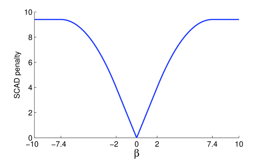
In this paper, we will use the SCAD penalty for our extensions of SIS and ISIS whenever necessary. The SCAD function is a quadratic spline and symmetric around the origin. It can be defined in terms of its first order derivative
for some and . Here is a parameter and Fan and Li (2001) recommend to use based on a Bayesian argument. The SCAD penalty is plotted in Figure 1 for and . The SCAD penalty is non-convex, leading to non-convex optimization. For the non-convex SCAD penalized optimization, Fan and Li (2001) proposed the local quadratic approximation; Zou and Li (2008) proposed the local linear approximation; Wu and Liu (2009) presented the difference convex algorithm. In this work, whenever necessary we use the local linear approximation algorithm to solve the SCAD penalized optimization.
4 SIS and ISIS for Cox’s proportional hazard model
The penalty based variable selection techniques work great with a moderate number of covariates. However their usefulness is limited while dealing with an ultra-high dimensionality as shown in Fan and Lv (2008). In the linear regression case, Fan and Lv (2008) proposed to rank covariates according to the absolute value of their marginal correlation with the response variable and select the top ranked covariates. They provided theoretical result to guarantee that this simple correlation ranking retains all important covariates with high probability. Thus they named their method sure independence screening (SIS). In order to handle difficult problems such as the one with some important covariates being marginally uncorrelated with the response, they proposed iterative SIS (ISIS). ISIS begins with SIS, then it regresses the response on covariates selected by SIS and uses the regression residual as a “working” response to recruit more covariates with SIS. This process can be repeated until some convergence criterion has been met. Empirical improvement over SIS has been observed for ISIS. In order to increase the power of the sure independence screening technique, Fan, Samworth and Wu (2009) has extended SIS and ISIS to more general models such as generalized linear models, robust regression, and classification and made several important improvements. We now extend the key idea of SIS and ISIS to handle Cox’s proportional hazards model.
Let be the index set of the true underlying sparse model, namely, , where s are the true regression coefficients in the Cox’s proportional hazards model (2.1).
4.1 Ranking by marginal utility
First let us review the definition of sure screening property.
Definition 1 (Sure Screening Property).
We say a model selection procedure satisfies sure screening property if the selected model with model size includes the true model with probability tending to one.
For each covariate (), define its marginal utility as the maximum of the partial likelihood of the single covariate:
Here is the -th element of , namely . Intuitively speaking, the larger the marginal utility is, the more information the corresponding covariate contains the information about the survival outcome. Once we have obtained all marginal utilities for , we rank all covariates according to their corresponding marginal utilities from the largest to the smallest and select the top ranked covariates. Denote by the index set of these covariates that have been selected.
The index set is expected to cover the true index set with a high probability, especially when we use a relative large . This is formally shown by Fan and Lv (2008) for the linear model with Gaussian noise and Gaussian covariates and significantly expanded by Fan and Song (2010) to generalized linear models with non-Gaussian covariates. The parameter is usually chosen large enough to ensure the sure screening property. However the estimated index set may also include a lot of unimportant covariates. To improve performance, the penalization based variable selection approach can be applied to the selected subset of the variables to further delete unimportant variables. Mathematically, we then solve the following penalized partial likelihood problem:
where denotes a sub-vector of with indices in and similarly for . It will lead to sparse regression parameter estimate . Denote the index set of nonzero components of by , which will serve as our final estimate of .
4.2 Conditional feature ranking and iterative feature selection
Fan and Lv (2008) pointed out that SIS can fail badly for some challenging scenarios such as the case that there exist jointly related but marginally unrelated covariates or jointly uncorrelated covariates having higher marginal correlation with the response than some important predictors. To deal with such difficult scenarios, iterative SIS (ISIS) has been proposed. Comparing to SIS which is based on marginal information only, ISIS tries to make more use of joint covariates’ information.
The iterative SIS begins with using SIS to select an index set , upon which a penalization based variable selection step is applied to get regression parameter estimate . A refined estimate of the true index set is obtained and denoted by , the index set corresponding to nonzero elements of .
As in Fan, Samworth and Wu (2009), we next define the conditional utility of each covariate that is not in as follows:
This conditional utility measures the additional contribution of the th covariate given that all covariates with indices in have been included in the model.
Once the conditional utilities have been defined for each covariate that is not in , we rank them from the largest to the smallest and select these covariates with top rankings. Denote the index set of these selected covariates by . With having been identified, we minimize
| (4.1) | |||
with respect to to get sparse estimate . Denote the index set corresponding to nonzero components of to be , which is our updated estimate of the true index set . Note that this step can delete some variables that were previously selected. This idea was proposed in Fan et al. (2009) and is an improvement of the idea in Fan and Lv (2008).
The above iteration can be repeated until some convergence criterion is reached. We adopt the criterion of either having identified covariates or for some .
4.3 New variants of SIS and ISIS for reducing FSR
Fan, Samworth and Wu (2009) noted that the idea of sample spliting can also be used to reduce the false selection rate. Without loss of generality, we assume that the sample size is even. We randomly split the sample into two halves. Then apply SIS or ISIS separately to the data in each partition to obtain two estimates and of the true index set . Both these two estimates could have high FSRs because they are based on a simple and crude screening method. Yet each of them should include all important covariates with high probabilities. Namely, important covariates should appear in both sets with probability tending to one asymptotically. Define a new estimate by intersection . The new estimate should include all important covaraites with high probability as well due to properties of each individual estimate. However by construction, the number of unimportant covariates in the new estimate is much smaller. The reason is that, in order for an unimportant covariate to appear in , it has to be included in both and randomly.
For the new variant method based on random splitting, Fan, Samworth and Wu (2009) obtained some non-asymptotic probability bound for the event that unimportant covaraites are included in the intersection for any natural number under some exchangeability condition on all unimportant covariates. The probability bound is decreasing in the dimensionality, showing a “blessing of dimensionality”. Please consult Fan, Samworth and Wu (2009) for more details. We want to remark that their theoretical bound is applicable to our setting as well while studying time-to-event data because theoretical bound is based on splitting the sample into two halves and only requires the independence between these two halves.
While defining new variants, we may use the same as used in the original SIS and ISIS. However it will lead to a very aggressive screening. We call the corresponding variant the first variant of (I)SIS. Alternatively, in each step we may choose larger and to ensure that their intersection has covariates, which is called the second variant. The second variant ensures that there are at least covariates included before applying penalization in each step and is thus much less aggressive. Numerical examples will be used to explore their performance and prefer to the first variant.
5 Simulation
5.1 Design of simulations
In this section, we conduct simulation studies to show the power of the (I)SIS and its variants by comparing them with LASSO (Tibshirani, 1997) in the Cox’s proportional hazards model. Here the regularization parameter for LASSO is tuned via five fold cross validation. Most of the settings are adapted from Fan and Lv (2008) and Fan, Samworth and Wu (2009). Four different configurations are considered with and . And two of them are revisited with a different pair of sample size and dimensionality . Covariates in different settings are generated as follows.
-
Case
1: are independent and identically distributed random variables.
-
Case
2: are multivariate Gaussian, marginally , and with serial correlation if . Here we take .
-
Case
3: are multivariate Gaussian, marginally , and with correlation structure for all and if and are distinct elements of .
-
Case
4: are multivariate Gaussian, marginally , and with correlation structure for all , for all , and if and are distinct elements of .
-
Case
5: Same as Case 2 except and .
-
Case
6: Same as Case 4 except and .
Here, Case 1 with independent predictors is the most straightforward for variable selection. In Cases 2-6, however, we have serial correlation such that does not decay as increases. We will see later that for Cases 3, 4 and 6, the true coefficients are specially chosen such that the response is marginally independent but jointly dependent of . We therefore expect variable selection in these situations to be much more challenging, especially for the non-iterated versions of SIS. Notice that in the asymptotic theory of SIS in Fan and Lv (2008), this type of dependence is ruled out by their Condition (4).
In our implementation, we choose for both the vanilla version of SIS (Van-SIS) and the second variant (Var2-SIS). For the first variant (Var1-SIS), however, we use (note that since the selected variables for the first variant are in the intersection of two sets of size , we typically end up with far fewer than variables selected by this method). For any type of SIS or ISIS, we apply SCAD with these selected predictors to get a final estimate of the regression coefficients at the end of the screening step. Whenever necessary, the BIC is used to select the best tuning parameter in the regularization framework.
In all setting, the censoring time is generated from exponential distribution with mean . This corresponds to choosing the baseline hazard function for . The true regression coefficients and censoring rate in each of the six cases are as follows:
-
Case
1: , and for . The corresponding censoring rate is 33%.
-
Case
2: The coefficients are the same as Case 1. The corresponding censoring rate is 27%.
-
Case
3: , and for . The corresponding censoring rate is 30%.
-
Case
4: and for . The corresponding censoring rate is 31%.
-
Case
5: , and for . The corresponding censoring rate is 23%.
-
Case
6: The coefficients are the same as Case 4. The corresponding censoring rate is 36%.
In Cases 1, 2 and 5 the coefficients were chosen randomly, and were generated as with and with probability 0.5 and -1 with probability 0.5, independent of . For Cases 3, 4, and 6, the choices ensure that even though , we have that and are marginally independent. The fact that is marginally independent of the response is designed to make it difficult for the common independent learning to select this variable. In Cases 4 and 6, we add another important variable with a small coefficient to make it even more difficult.
5.2 Results of simulations
We report our simulation results based on 100 Monte Carlo repetitions for each setting in Tables 1-7. To present our simulation results, we use several different performance measures. In the rows labeled and , we report the median and squared estimation errors and , respectively, where the median is over the 100 repetitions. In the row with label , we report the proportion of the 100 repetitions that the (I)SIS procedure under consideration includes all of the important variables in the model, while the row with label reports the corresponding proportion of times that the final variables selected, after further application of the SCAD penalty, include all of the important ones. We also report the median model size (MMS) of the final model among 100 repetitions in the row labeled MMS.
| Case 1: independent covariates | |||||||
| Van-SIS | Van-ISIS | Var1-SIS | Var1-ISIS | Var2-SIS | Var2-ISIS | LASSO | |
| 0.79 | 0.57 | 0.73 | 0.61 | 0.76 | 0.62 | 4.23 | |
| 0.13 | 0.09 | 0.15 | 0.1 | 0.15 | 0.1 | 0.98 | |
| 1 | 1 | 0.99 | 1 | 0.99 | 1 | – | |
| 1 | 1 | 0.99 | 1 | 0.99 | 1 | 1 | |
| MMS | 7 | 6 | 6 | 6 | 6 | 6 | 68.5 |
| Case 2: Equi-correlated covariates with | |||||||
| Van-SIS | Van-ISIS | Var1-SIS | Var1-ISIS | Var2-SIS | Var2-ISIS | LASSO | |
| 2.2 | 0.64 | 4.22 | 0.8 | 3.95 | 0.78 | 4.38 | |
| 1.74 | 0.11 | 4.71 | 0.29 | 4.07 | 0.28 | 0.98 | |
| 0.71 | 1 | 0.42 | 0.99 | 0.46 | 0.99 | – | |
| 0.71 | 1 | 0.42 | 0.99 | 0.46 | 0.99 | 1 | |
| MMS | 7 | 6 | 6 | 6 | 7 | 6 | 57 |
We report results of Cases 1 and 2 in Table 1. Recall that the covariates in Case 1 are all independent. In this case, the Van-SIS performs reasonably well. Yet, it does not perform well for the dependent case, Case 2. Note the only difference between Case 1 and Case 2 is the covariance structure of the covariates. For both cases, vanilla-ISIS and its second variant perform very well. It is worth noticing that the ISIS improves significantly over SIS, when covariates are dependent, in terms of both the probability of including all the true variables and in reducing the estimation
error. This comparison indicates that the ISIS performs much better when there is serious correlation among covariates.
While implementing the LASSO penalized Cox’s proportional hazards model, we adapted the Fortran source code in the R package “glmpath.” Recall that the objective function in the LASSO penalized Cox’s proportional hazards model is convex and nonlinear. What the Fortran code does is to call a MINOS subroutine to solve the corresponding nonlinear convex optimization problem. Here MINOS is an optimization software developed by Systems Optimization Laboratory at Stanford University. This nonlinear convex optimization problem is much more complicated than a general quadratic programming problem. Thus generally it takes much longer time to solve, especially so when the dimensionality is high as confirmed by Table 3. However the algorithm we used does converge as the objective function is strictly convex.
Table 1 shows that LASSO has the sure screening property as the ISIS, however, the median model size is ten times as large as that of ISIS. As a consequence, it also has larger estimation errors in terms of and . The fact that the median absolute deviation error is much larger than the median square error indicates that the LASSO selects many small nonzero coefficients for those unimportant variables. This is also verified by the fact that LASSO has a very large median model size. The explanation is the bias issue noted by Fan and Li (2001). In order for LASSO to have a small bias for nonzero coefficients, a smaller should be chosen. Yet, a small recruits many small coefficients for unimportant variables. For Case 2, the LASSO has a similar performance as in Case 1 in that it includes all the important variables but has a much larger model size.
| Case 3: An important predictor that is independent of survival time | |||||||
| Van-SIS | Van-ISIS | Var1-SIS | Var1-ISIS | Var2-SIS | Var2-ISIS | LASSO | |
| 20.1 | 1.03 | 20.01 | 0.99 | 20.09 | 1.08 | 20.53 | |
| 94.72 | 0.49 | 100.42 | 0.47 | 94.77 | 0.55 | 76.31 | |
| 0 | 1 | 0 | 1 | 0 | 1 | – | |
| 0 | 1 | 0 | 1 | 0 | 1 | 0.06 | |
| MMS | 13 | 4 | 8 | 4 | 13 | 4 | 118.5 |
| Case 4: Two very hard variables to be selected. | |||||||
| Van-SIS | Van-ISIS | Var1-SIS | Var1-ISIS | Var2-SIS | Var2-ISIS | LASSO | |
| 20.87 | 1.15 | 20.95 | 1.4 | 20.96 | 1.41 | 21.04 | |
| 96.46 | 0.51 | 102.14 | 1.77 | 97.15 | 1.78 | 77.03 | |
| 0 | 1 | 0 | 0.99 | 0 | 0.99 | – | |
| 0 | 1 | 0 | 0.99 | 0 | 0.99 | 0.02 | |
| MMS | 13 | 5 | 9 | 5 | 13 | 5 | 118 |
Results of Cases 3 and 4 are reported in Table 2. Note that, in both cases, the design ensures that is marginally independent of but jointly dependent on . This special design disables the SIS to include in the corresponding identified model as confirmed by our numerical results. However, by using ISIS, we are able to select for each repetition. Surprisingly, LASSO rarely includes even if it is not a marginal screening based method. Case 5 is even more challenging. In addition to the same challenge as case 4, the coefficient is 3 times smaller than the first four variables. Through the correlation with the first 4 variables, unimportant variables have a larger marginal utility with than . Nevertheless, the ISIS works very well and demonstrates once more that it uses adequately the joint covariate information.
| Case 1 | Case 2 | Case 3 | Case 4 | |
|---|---|---|---|---|
| Van-ISIS | 379.29 | 213.44 | 402.94 | 231.68 |
| LASSO | 37730.82 | 26348.12 | 46847 | 28157.71 |
We also compare the computational cost of van-ISIS and LASSO in Table 3 for Cases 1-4. Table 3 shows that it takes LASSO several hours for each repetition, while van-ISIS can finish it in just several minutes. This is a huge improvement. For this reason, for Cases 5 and 6 where , we only report the results for ISIS since it takes LASSO over several days to complete a single repetition. Results of Cases 5 and 6 are reported in Table 4. The table demonstrates similar performance as Cases 2 and 4 even with more covariates.
| Case 5: The same as case 2 with and | ||||||
| Van-SIS | Van-ISIS | Var1-SIS | Var1-ISIS | Var2-SIS | Var2-ISIS | |
| 1.53 | 0.52 | 3.55 | 0.55 | 2.95 | 0.51 | |
| 0.9 | 0.07 | 3.48 | 0.08 | 2.5 | 0.07 | |
| 0.82 | 1 | 0.39 | 1 | 0.5 | 1 | |
| 0.82 | 1 | 0.39 | 1 | 0.5 | 1 | |
| MMS | 8 | 6 | 6 | 6 | 7 | 6 |
| Case 6: The same as case 4 with and . | ||||||
| Van-SIS | Van-ISIS | Var1-SIS | Var1-ISIS | Var2-SIS | Var2-ISIS | |
| 20.88 | 0.99 | 20.94 | 1.1 | 20.94 | 1.29 | |
| 93.53 | 0.39 | 104.76 | 0.44 | 94.02 | 1.35 | |
| 0 | 1 | 0 | 1 | 0 | 0.99 | |
| 0 | 1 | 0 | 1 | 0 | 0.99 | |
| MMS | 16 | 5 | 8 | 5 | 16 | 5 |
To conclude the simulation section, we demonstrate the difficulty of our simulated models by showing the distribution, among 100 simulations, of the minimum -statistic for the estimates of the true nonzero regression coefficients in the oracle model with only true important predictors included. More explicitly, during each repetition of each simulation setting, we pretend to know the index set the true underlying sparse model, fit the Cox’s proportional hazards model using only predictors with indices in by calling function “coxph” of R package “survival”, and report the smallest absolute value of the -statistic for the regression estimates. For example, for case 1, the model size is only 6 and the minimum -statistic is computed based on these 6 estimates for each simulation. This shows the difficulty to recover all significant variables even in the oracle model with the minimum model size. The corresponding boxplot for each case is shown in Figure 2. To demonstrate the effect of including unimportant variables, the minimum -statistic for the estimates of the true nonzero regression coefficients is recalculated and shown by the boxplots in Figure 3 for the model with the true important variables and 20 unimportant variables.


As expected, cases 1 and 2 are relatively easy cases, whereas cases 3 and 4 are relatively harder in the oracle model. When we are not in the oracle model with 20 noisy variables are added, the difficulty increases as shown in Figure 3. It has more impact on cases 3, 4 and 6.
6 Real data
In this section, we use one real data set to demonstrate the power of the proposed method. The Neuroblastoma data set is due to Oberthuer et al. (2006). It was used in Fan, Samworth and Wu (2009) for classification studies. Neuroblastoma is an extracranial solid cancer. It is most common in childhood and even in infancy. The annual number of incidences is about several hundreds in the United States. Neuroblastoma is a malignant pediatric tumor originating from neural crest elements of the sympathetic nervous system.
The study includes 251 patients of the German Neuroblastoma Trials NB90-NB2004, who were diagnosed between 1989 and 2004. The patients’ ages range from 0 to 296 months at diagnosis with a median age of 15 months. Neuroblastoma specimens of these 251 patients were analyzed using a customized oligonucleotide microarray. The goal is to study the association of gene expression with variable clinical information such as survival time and 3-year event free survival, among others.

We obtained the neuroblastoma data from the MicroArray Quality Control phase-II (MAQC-II) project conducted by the Food Drug Administration (FDA). The complete data set includes gene expression at 10,707 probe sites. It also includes the survival information of each patient. In this example, we focus on the overall survival. There are five outlier arrays. After removing outlier arrays from our consideration, there are 246 patients. The (overall) survival information is available all of these 246 patients. The censoring rate is 205/246, which is very heavy. The survival times of those 246 patients are summarized in Figure 4.
As real data are always complex, there may be some genes that are marginally unimportant but work jointly with other genes. Thus it is more appropriate to apply iterative SIS instead of SIS, since the former is more powerful. We standardize each predictor to have mean zero and standard deviation 1 and apply van-ISIS to the standardized data with . ISIS followed with SCAD penalized Cox regression selects 8 genes with probe site names: A_23_P31816, A_23_P31816, A_23_P31816, A_32_P424973, A_32_P159651, Hs61272.2, Hs13208.1, and Hs150167.1.
| Probe ID | estimated coefficient | standard error | p-value |
|---|---|---|---|
| A_23_P31816 | 0.864 | 0.203 | 2.1e-05 |
| A_23_P31816 | -0.940 | 0.314 | 2.8e-03 |
| A_23_P31816 | -0.815 | 1.704 | 6.3e-01 |
| A_32_P424973 | -1.957 | 0.396 | 7.8e-07 |
| A_32_P159651 | -1.295 | 0.185 | 2.6e-12 |
| Hs61272.2 | 1.664 | 0.249 | 2.3e-11 |
| Hs13208.1 | -0.789 | 0.149 | 1.1e-07 |
| Hs150167.1 | 1.708 | 1.687 | 3.1e-01 |

Now we try to provide some understanding to the significance of these selected genes in predicting the survival information in comparison to other genes that are not selected. We first fitted the Cox’s proportional hazard model with all these eight genes. Estimated coefficients are given in Table 5, estimated baseline survival function is plotted in Figure 5, and the corresponding log-(partial)likelihood (2.4) is -129.3517. The log-likelihood corresponding to the null model without any predictor is -215.4561. A test shows the obvious significance of the model with the eight selected genes. Table 5 shows that there are two estimated coefficients that are statistically insignificant at ..
Next for each one of these eight genes, we remove it, fit Cox’s proportional hazard model with the other seven genes, and get the corresponding log-likelihood. The eight log-likelihoods are -137.5785, -135.1846, -129.4621, -142.4066, -156.4644, -158.3799, -141.0432, and -129.8390. Their average is -141.2948, a decrease of log-likelihood by 11.9431, which is very significant with reduction one gene (the reduction of the degree of freedom by 1). In comparison to the model with the eight selected genes, tests shows significance for all selected genes except A_23_P31816 and Hs150167.1. This matches the p-values reported in Table 5.
Finally we randomly select 2 genes out of the genes that are not selected, fit the Cox’s proportional hazard model with the above eight genes plus these two randomly selected genes, and record the corresponding log-likelihood. We repeat this process 20 times. We find that the average of these 20 new log-likelihoods is -128.3933, an increase of the log-likelihood merely by 0.9584 with two extra variables included. Comparing to the model with the eight selected genes, test shows no significance for the model corresponding to any of the 20 repetitions.
The above experiments show that the selected 8 genes are very important. Deleting one reduces a lot of log-likelihood, while adding two random genes do not increase very much the log-likelihood.
7 Conclusion
We have developed a variable selection technique for the survival analysis with the dimensionality that can be much larger than sample size. The focus is on the iterative sure independence screening, which iteratively applies a large-scale screening that filters unimportant variables by using the conditional marginal utility, and a moderate-scale selection by using penalized partial likelihood method, which selects further the unfiltered variables. The methodological power of the vanilla ISIS has been demonstrated via carefully designed simulation studies. It has sure independence screening with very small false selection. Comparing with the version of LASSO we used, it is much more computationally efficient and far more specific in selection important variables. As a result, it has much smaller absolute deviation error and mean square error.
References
- Cox (1972) Cox, D. R. (1972). Regression models and life-tables (with discussion). Journal of the Royal Statistical Society Series B, 34 187–220.
- Cox (1975) Cox, D. R. (1975). Partial likelihood. Biometrika, 62 269–76.
- Fan et al. (2010) Fan, J., Feng, Y. and Song, R. (2010). Nonparametric independence screening in sparse ultra-high dimensional additive models. Submitted.
- Fan and Li (2001) Fan, J. and Li, R. (2001). Variable selection via nonconcave penalized likelihood and its oracle properties. Journal of the American Statistical Association, 96 1348–1360.
- Fan and Li (2002) Fan, J. and Li, R. (2002). Variable selection for cox’s proportional hazards model and frailty model. Annals of Statistics, 30 74–99.
- Fan and Lv (2008) Fan, J. and Lv, J. (2008). Sure independence screening for ultrahigh dimensional feature space (with discussion). Journal of the Royal Statistical Society Series B, 70 849–911.
- Fan et al. (2009) Fan, J., Samworth, R. and Wu, Y. (2009). Ultrahigh dimensional variable selection: beyond the lienar model. Journal of Machine Learning Research. To appear.
- Fan and Song (2010) Fan, J. and Song, R. (2010). Sure independence screening in generalized linear models with np-dimensionality. The Annals of Statistics, to appear.
- Faraggi and Simon (1998) Faraggi, D. and Simon, R. (1998). Bayesian variable selection method for censored survival data. Biometrics, 54 1475–5.
- Ibrahim et al. (1999) Ibrahim, J. G., Chen, M.-H. and Maceachern, S. N. (1999). Bayesian variable selection for proportional hazards models. Canandian Journal of Statistics, 27 701–17.
- Klein and Moeschberger (2005) Klein, J. P. and Moeschberger, M. L. (2005). Survival analysis. 2nd ed. Springer.
- Li and Dicker (2009) Li, Y. and Dicker, L. (2009). Dantzig selector for censored linear regression. Technical report, Harvard University Biostatistics.
- Oberthuer et al. (2006) Oberthuer, A., Berthold, F., Warnat, P., Hero, B., Kahlert, Y., Spitz, R., Ernestus, K., König, R., Haas, S., Eils, R., Schwab, M., Brors, B., Westermann, F. and Fischer, M. (2006). Customized oligonucleotide microarray gene expressionbased classification of neuroblastoma patients outperforms current clinical risk stratification. Journal of Clinical Oncology, 24 5070–5078.
- Sauerbrei and Schumacher (1992) Sauerbrei, W. and Schumacher, M. (1992). A bootstrap resampling procedure for model building: Application to the cox regression model. Statistics in Medicine, 11 2093–2109.
- Tibshirani (1997) Tibshirani, R. (1997). The lasso method for variable selection in the cox model. Statistics in Medicine, 16 385–95.
- Tibshirani (1996) Tibshirani, R. J. (1996). Regression shrinkage and selection via the lasso. Journal of the Royal Statistical Society, Series B, 58 267–288.
- Wu and Liu (2009) Wu, Y. and Liu, Y. (2009). Variable selection in quantile regression. Statistica Sinica, 19 801–817.
- Zhang (2009) Zhang, C.-H. (2009). Penalized linear unbiased selection. Ann. Statist. To appear.
- Zhang and Lu (2007) Zhang, H. H. and Lu, W. (2007). Adaptive lasso for cox’s proportional hazards model. Biometrika, 94 691–703.
- Zou (2006) Zou, H. (2006). The adaptive lasso and its oracle properties. Journal of the American Statistical Association, 101 1418–1429.
- Zou and Li (2008) Zou, H. and Li, R. (2008). One-step sparse estimates in nonconcave penalized likelihood models (with discussion). Annals of Statistics, 36 1509–1566.
- Zou and Hastie (2005) Zou, H. and Hastie, T. (2005). Regularization and variable selection via the elastic net. Journal of the Royal Statistical Society, Series B, 67 301–320.