High-harmonic generation in diatomic molecules: a quantum-orbit analysis of the interference patterns

In general, the strong-field approximation (SFA) consists in neglecting the influence of the laser field when the electron is bound, the atomic or molecular binding potential when the electron is in the continuum and the internal structure of the system in question, i.e., contributions from its excited bound states. The SFA transition amplitude for high-order harmonic generation reads, in the specific formulation of Ref. hhgsfa and in atomic units,

with the action

and the prefactors $d_{\mathrm{rec}}(\mathbf{\tilde{p}}(t))=\left\langle\mathbf{\tilde{p}}(t)\right|\mathcal{O}_{\mathrm{dip}}.\mathbf{e}_{x}\left|\psi_{0}\right\rangle$ and $d_{\mathrm{ion}}(\mathbf{\tilde{p}}(t^{\prime}))=\left\langle\mathbf{\tilde{p}}(t^{\prime})\right|H_{\mathrm{int}}\mathbf{(}t^{\prime}\mathbf{)}\left|\psi_{0}\right\rangle.$ In the above equations, $\mathcal{O}_{\mathrm{dip}}$, $\mathbf{e}_{x}$, $H_{\mathrm{int}}\mathbf{(}t^{\prime}\mathbf{),}$ $I_{p},$ and $\Omega$ denote the dipole operator, the laser-polarization vector, the interaction with the field, the ionization potential, and the harmonic frequency, respectively. The explicit expressions for $\mathbf{\tilde{p}}(t)$ are gauge dependent, and will be given below. The above-stated equation describes a physical process in which an electron, initially in a field-free bound-state $\left|\psi_{0}\right\rangle$, is coupled to a Volkov state $\left|\mathbf{\tilde{p}}(t^{\prime})\right\rangle$ by the interaction $H_{\mathrm{int}}\mathbf{(}t^{\prime}\mathbf{)}$ of the system with the field. Subsequently, it propagates in the continuum and is driven back towards its parent ion, with which it recombines at a time $t$, emitting high-harmonic radiation of frequency $\Omega.$ In Eq. (1), additionally to the above-mentioned assumptions, the further approximation of considering only transitions from a bound state to a Volkov state in the dipole moment has been made. In the single atom case, this has been justified by the fact that the remaining contributions, from the so-called “continuum-to-continuum” transitions, were very small. For a discussion of the various formulations of the SFA see, e.g., BLM94 ; hhgsfa ; atisfa and in particular BeckLew97 .

Due to the fact that it can be carried out almost entirely analytically, the SFA is a very powerful approach. It possesses, however, the main drawback of being gauge-dependent (for general discussions see, e.g., Ref. FKS96 , and for the specific case of molecules, Ref. PRACL2006 ). Apart from the obvious fact that the interaction Hamiltonians $H_{\mathrm{int}}(t^{\prime})$, which are present in $d_{\mathrm{ion}}(\mathbf{\tilde{p}}(t^{\prime}))$, are different in the length and velocity gauges footngauge , in most computations where the SFA is employed, field-free bound states are taken, which are not gauge equivalent. Indeed, a field-free bound state $\left|\psi_{0}^{(L)}\right\rangle$ in the length gauge would be gauge equivalent to the field-dressed state $\left|\psi_{0}^{(V)}\right\rangle=\chi_{v\leftarrow l}\left|\psi_{0}^{(L)}\right\rangle$ in the velocity gauge, with $\chi_{v\leftarrow l}=\exp[i\mathbf{A}(t)\cdot\mathbf{r}].$ Such a phase shift causes a translation $\mathbf{p\rightarrow p-A}(t)$ on a momentum eigenstate $\left|\mathbf{p}\right\rangle.$ Hence, for field-free bound states in both gauges it leads to different dipole matrix elements $d_{\mathrm{rec}}(\mathbf{\tilde{p}}(t))$ and $d_{\mathrm{ion}}(\mathbf{\tilde{p}}(t))$. Explicitly, in the length gauge $\mathbf{\tilde{p}}(t)=\mathbf{p}+\mathbf{A}(t)$, while in the velocity gauge $\mathbf{\tilde{p}}(t)=\mathbf{p}.$

For computations involving a single atom, the latter artifact can be avoided by placing the system at the origin of the coordinate system. For systems composed of several centers, such as molecules, however, this ambiguity will always be present. Indeed, in the literature, different results have been reported for molecular SFA computations in the velocity and in the length gauge PRACL2006 ; DM2006 ; Madsen ; Usachenko . In recent, modified versions of the length-gauge SFA, this problem has been eliminated for ATI by considering the initial bound state $\left|\tilde{\psi}_{0}^{(L)}\right\rangle=\exp[-i\mathbf{A}(t^{\prime})\cdot\mathbf{r}]\left|\psi_{0}^{(L)}\right\rangle.$ Such a state is gauge-equivalent to a field-free bound state in the velocity gauge, and, physically, may be interpreted as a field-dressed state, in which the laser-field polarization is included dressedSFA ; DM2006 . For HHG, one may proceed in a similar way, with the main difference that the dressing should also be included in the final state, with which the electron recombines. In the dressed modified SFA, $\mathbf{\tilde{p}}(t)=\mathbf{p}$.

We will now apply the SFA to a diatomic molecule. For this purpose, we will consider the simplest scenario, namely a one-electron system and frozen nuclei. Furthermore, we will assume that the molecular orbital from which the electron is released and with which it may recombine is a linear combination of atomic orbitals (LCAO approximation). Explicitly, the molecular bound-state wave function reads

where $\epsilon=\pm 1,\mathbf{r}_{1}=\mathbf{r}-\mathbf{R}/2,$ and $\mathbf{r}_{2}=\mathbf{r}+\mathbf{R}/2$ denote the positions of the centers $C_{1}$ and $C_{2},$ respectively, and $C_{\psi}$ is a normalization constant.  For homonuclear molecules, which we will consider here, $\psi_{0}^{(1)}=\psi_{0}^{(2)}=\varphi_{0}$. The positive and negative signs for $\epsilon$ correspond to bonding and antibonding orbitals, respectively. Within this context, there exist two main approaches for computing high-order harmonic spectra, which will be discussed next.

We will commence by considering the single-center action (2) and the prefactors discussed in the previous section. In Fig. 1, we depict high-harmonic spectra computed for a wide range of internuclear distances, employing the prefactor (15) or the modified expression (20), for which the linear term in $R_{x}$ is absent [upper and lower panel, respectively]. The figure illustrates how the linear term masks the interference patterns. In fact, for a.u. $1\leq R\leq 3$ a.u., it counterbalances the influence of the purely trigonometric term, and no clear minima and maxima are observed. As the internuclear distance increases, this term starts to play a dominant role, displacing the maxima and minima away from the double-slit condition (17). Furthermore, it seems that the patterns become more distinct with increasing harmonic order.

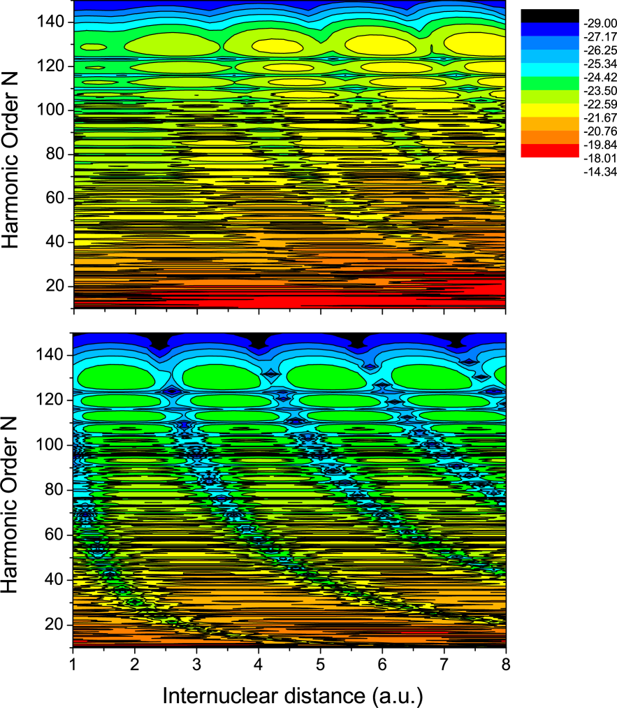
A rough estimate of the influence of each term in (15) on the spectra agrees with Fig. 1. Since the trigonometric functions in (15) are bounded, the ratio between the maxima caused by each term will be  $\varsigma=R|\cos\theta\phi(\mathbf{\tilde{p}})/(2\partial_{p_{x}}\phi(\mathbf{\tilde{p}}))|$, where $\theta$ is the alignment angle and $\phi(\mathbf{\tilde{p}})$ is given by Eq. (14). If $\varsigma\simeq 1$, the maxima will possess the same order of magnitude and there will be no noticeable modulation, while if $\varsigma<1$ the double-slit physical picture may still be reproduced. For $\varsigma>1,$ however, one expects that the linear term in $R$ will prevail. Hence, the critical value for the internuclear distance is $R_{c}=2|\sec\theta\partial_{p_{x}}\phi(\mathbf{\tilde{p}})/\phi(\mathbf{\tilde{p}})|$. This expression depends on the bound states with which the electron recombines, and also on the harmonic energy. For instance, specifically for $1s$ states, $R_{c}\sim 4{\tilde{p}_{x}}\sec\theta/(\mathbf{\tilde{p}}^{2}+2I_{p}).$ Above the ionization threshold, according to Eq. (6), $R_{c}\sim 2\tilde{p}_{x}\sec\theta/\Omega$. Hence, one expects the linear term to be more prominent as the harmonic energy increases, leading to clearer, though incorrect, patterns. In order to avoid such problems, we will employ the prefactor (20) throughout.

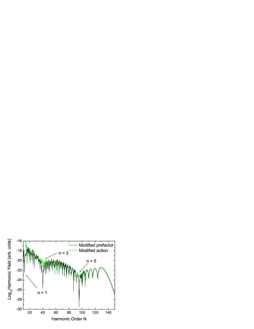
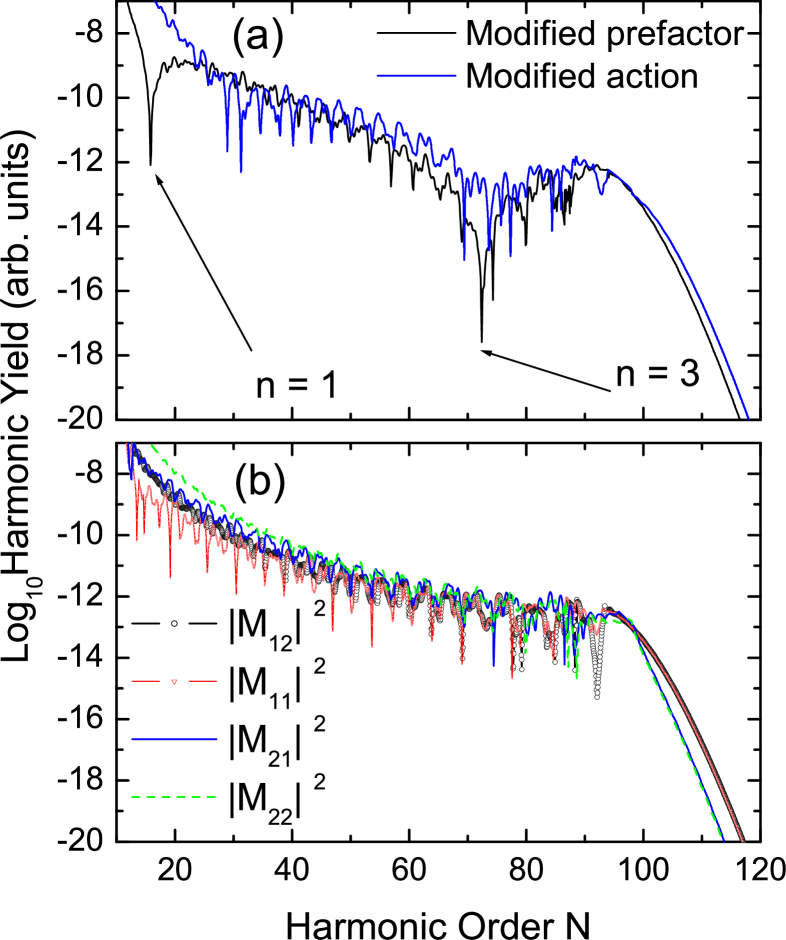
In Fig. 2, we compare spectra computed using either the pre-factor (20) or modified saddle-point equations. Both spectra are very similar, with maxima and minima at harmonic frequencies $\Omega=I_{p}+n^{2}\pi^{2}/(2R_{x}^{2})$, as expected from the double-slit condition. This similarity holds not only for the gross features, but, additionally, for the substructure caused by other types of quantum interference. Close to the minima, however, the yield from the latter case is larger. Nevertheless, the very good overall agreement shows that, in fact, the patterns obtained can also be interpreted as the result of the quantum interference between different types of electron orbits.

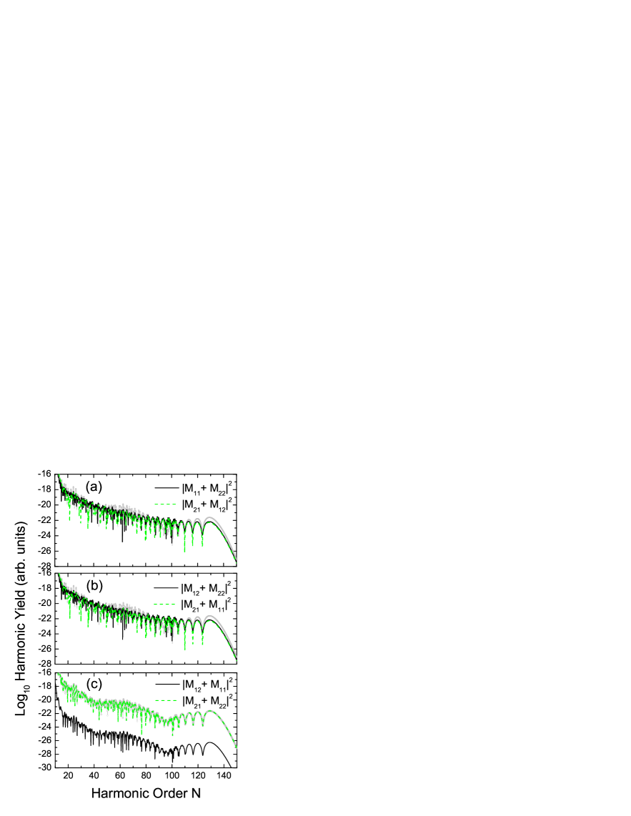
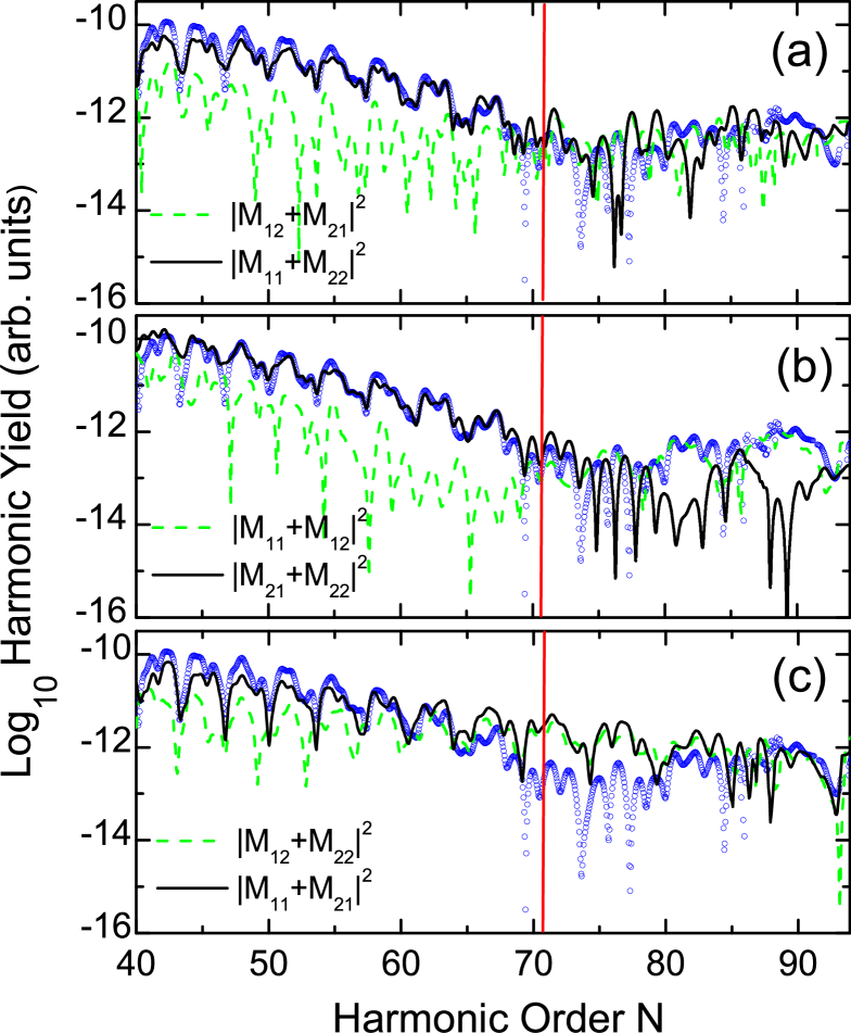
In order, however, to identify which sets of orbits cause the dips and the maxima, we will analyze the interference between their individual contributions. Such results are shown in Fig. 3. In the upper panels, we present the spectra computed from topologically similar sets of orbits, i.e., from processes involving only one, or two centers [panel 3.(a)]. In this case, the main interference patterns are absent. This strongly suggests that they are due to the quantum interference of topologically different sets of orbits: the orbits along which an electron leaves and returns to the same center, and those along which it reaches the continuum at one center and recombines with the other. Physically, this could be attributed to the fact that, in this case, there would be an appreciable phase difference between the two sets of orbits, since the latter are much longer than the former. This phase difference would cause the overall modulation.

Hence, there are two remaining possibilities. Concretely, the modulation can be due to the quantum interference either between processes in which the electron leaves from different centers and recombines with the same center (i.e., between the orbits which start at $C_{j}$ and end at $C_{\nu}$, with $\nu\neq j,$ and those starting and ending at $C_{\nu}$, and $j=1,2$), or between those in which an electron starts at the same center and recombines with different centers (i.e., the electron is ejected at $C_{j}$ and recombines at $C_{\nu}$, $\nu\neq j,$ or it is freed and recombines at $C_{j}$, with $j=1,2$). In panel 3.(b), we consider the former processes, whereas in panel 3.(c) we depict the latter. Interestingly, only in case the electron leaves from the same center, the interference patterns are present. Furthermore, there is a difference in roughly four orders of magnitude between the two types of contributions. Such a difference is absent in the other cases. Additionally, the full contributions to the yield are practically indistinguishable from the transition probability $|M_{21}+M_{22}|^{2},$ from the orbits starting at $C_{2}.$

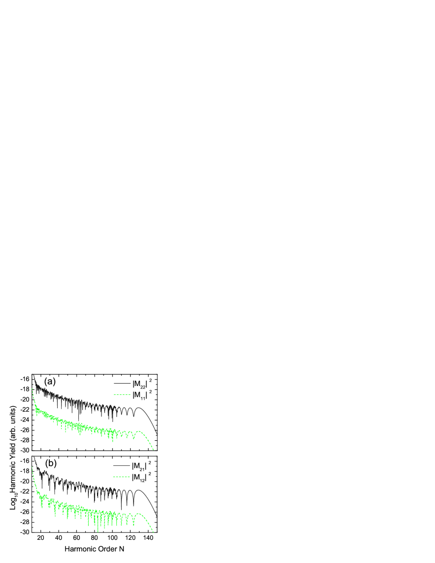
In order to understand this better, one must have a closer look at the individual contributions from different sets of orbits, and, in particular their orders of magnitude. Such contributions, depicted in Panels (a) and (b) of Fig. 4, show that the transition probabilities $|M_{22}|^{2}$ and $|M_{21}|^{2},$ which correspond to the orbits starting from the center $C_{2},$ are roughly four orders of magnitude larger than $|M_{12}|^{2}$ and $|M_{11}|^{2}$, i.e., than those from the orbits starting at $C_{1}$. Therefore, it is not surprising that the yield is dominated by $|M_{21}+M_{22}|^{2}$ in the previous figure. Furthermore, these results exhibit no maxima and minima. Hence, they support the assumption that such features are due to the interference of different types of orbits. Finally, the contributions from orbits starting at the same center possess the same order of magnitude. This suggests that tunneling ionization is the main mechanism determining the relevance of a particular type of orbits to the spectra, and that are local differences in the barrier through which the electron must tunnel, depending on the center it starts from.

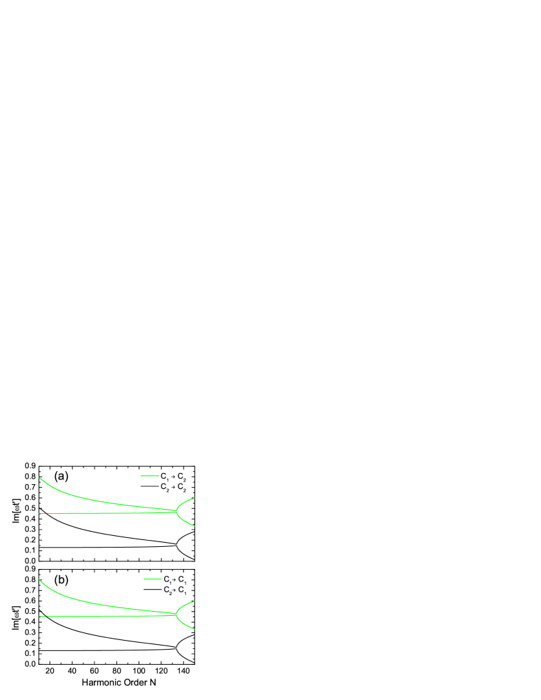
An inspection of the imaginary parts $\mathrm{Im}[t^{\prime}]$ of the start times provides additional insight into this problem. Due to the fact that tunneling ionization is a process which has no classical counterpart, this quantity is always non-vanishing, even if the energy range in question is lower than the maximal harmonic energy. The larger $\mathrm{Im}[t^{\prime}]$ is, the less probable it will be that tunneling ionization takes place. Such an interpretation has been successfully employed in FLSL2004 in order to determine the dominant pairs of orbits, in the context of nonsequential double ionization with few-cycle laser pulses, and will be also considered in this work. For that purpose, we will take the shortest pairs of orbits utilized in the computation of the transition probabilities in Fig. 4 and, for each case, display $\mathrm{Im}[t^{\prime}]$. These are the dominant pairs of orbits. The longer pairs have a less significant influence on the spectra, due to the spreading of the electronic wave packet spreading .

Such results are depicted in Fig. 5. Clearly, $\mathrm{Im}[t^{\prime}]$ is around four times larger for the orbits starting from the center $C_{1}$, as compared to those starting from $C_{2}.$ This means that, in order to reach the continuum, the electron must overcome a larger barrier if it comes from $C_{1}$. Since, roughly speaking, the ionization probability per unit time decreases exponentially with $\mathrm{Im}[t^{\prime}]$, one expects the contributions from the orbits starting from $C_{1}$ to be around four orders of magnitude smaller than those from the orbits starting at $C_{2}$. An inspection of Fig. 4 shows that this is indeed the case.

The above-stated effect could, however, be an artifact of the strong-field approximation in the length gauge. Indeed, the terms $\pm\mathbf{E}(t^{\prime})\cdot\mathbf{R}$ in the saddle-point equations (25) and (27) can be interpreted as potential energy shifts, due to the fact that the electron is displaced from the origin PRACL2006 ; DM2006 . Such terms increase or sink the potential barrier for $C_{1}$ or $C_{2},$ respectively, and, consequently, change the orders of magnitude in the contributions starting from different centers. Even though, as a whole, the results match those obtained by other means, their physical interpretation is controversial.

One may, however, avoid this problem by providing an additional pathway for the electron to reach the continuum. For that purpose, we shall superpose a time-delayed attosecond pulse train to the strong laser field, employing the model discussed in Sec. II.2.3 and in our previous work FSVL2006 ; FS2006 . The maximal harmonic energies for this specific model are strongly dependent on the time delay $t_{d}$ between the attosecond-pulse train the infra-red field, extending from the ionization potential, for $\phi=0.75\pi$ to $I_{p}+1.8U_{p}$, for $\phi=n\pi$. Furthermore, there exist many intermediate delays, for which a double plateau is present. This substructure may be detrimental to the identification and physical interpretation of the interference patterns. In order to avoid such problems, we will consider here vanishing time delay, i.e., $\phi=0.$

In Fig. 6, we depict the spectra obtained for a diatomic molecule subjected to such a field, assuming either a two-center prefactor and the single-center saddle-point equation (35), or the modified saddle point equations (36) [Fig. 6.(a)]. Both computations exhibit a minimum near the harmonic frequency $\Omega=71\omega$, in agreement with Eq. (17). If only the contributions $|M_{j\nu}|^{2}$ from the individual scattering scenarios are taken, such a minimum is absent [Fig. 6.(b)]. Therefore, it is due to interference effects between different sets of orbits. One should note that, in contrast to the purely monochromatic case, all contributions exhibit the same order of magnitude. This is due to the fact that, if the attosecond pulses are present, the electron is being ejected in the continuum with roughly the same probability, regardless of the center it left from.

The precise role of the various recombination scenarios is illustrated in Fig. 7. For clarity, we concentrate on the plateau region around the interference minimum. The main difference observed, with regard to the purely monochromatic case, is that the overall shape of the spectrum, and consequently its minimum, is due to the collective interference of several types of orbits. This is in contrast to the previous results, for which they were caused by the processes starting at a center $C_{j}$ and ending at different centers, i.e., $|M_{jv}+M_{jj}|^{2}$, with $\nu\neq j$ and $\nu,j$ $=(1,2)$. Indeed, a modulation is even present for the probability $|M_{11}+M_{22}|^{2}$ involving only one-center scenarios. This is shown in Fig. 7.(a), and contradicts the previously made assumption that such features are due to the interference between topologically different sets of orbits. In fact, it seems that the absence of overall maxima and minima for the one-center contributions, in the purely monochromatic case [Fig. 3.(a)], is due to the different orders of magnitude for $M_{11}$ and $M_{22}$ [c.f. Fig. 4.(a)].

Furthermore, one needs several different processes in order to obtain the correct position of the minimum. For instance, in Fig. 7.(a), the overall spectrum closely follows $|M_{11}+M_{22}|^{2}$ in the low-energy region. In the vicinity of the minimum and for higher energies, however, it follows neither such contrbutions nor $|M_{12}+M_{21}|^{2},$ from two-center processes. In Fig. 7.(b), where we display the contributions $|M_{jj}+M_{j\nu}|^{2}$, with $\nu\neq j$ and $\nu,j$ $=(1,2),$ from the orbits starting from the same center, the spectrum closely follows $|M_{21}+M_{22}|^{2}$ before the minimum, and $|M_{11}+M_{12}|^{2}$ after the minimum.

The remaining panel [Fig. 7.(c)] depicts the contributions from $|M_{\nu\nu}+M_{j\nu}|^{2}$ , with $\nu\neq j$ and $\nu,j$ $=(1,2)$, which give the orbits finishing at the same center. In this case, the interference minimum is absent. This is a strong evidence that the relevant condition for the presence of such features is that the orbits taken into account end at different centers, instead of being topologically different (which is the case for both Fig. 7.(b) and Fig. 7.(c)). Therefore, these results agree with the double-slit picture, which has been put across in doubleslit .

The additional attosecond pulses have the advantage of not introducing changes in the standard length-gauge SFA formulation. They modify, however, the physics of the problem, since they provide a different mechanism for the electron to reach the continuum. Clearly, there is also the possibility of eliminating the spurious potential energy shifts, by considering a different version of the SFA, such as the field-dressed length-gauge formulation proposed in DM2006 , or the velocity-gauge formulation.

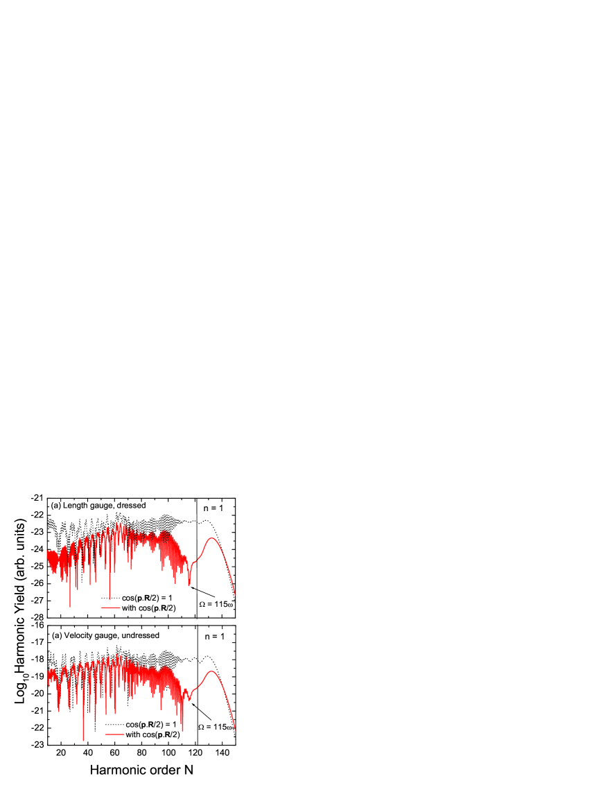
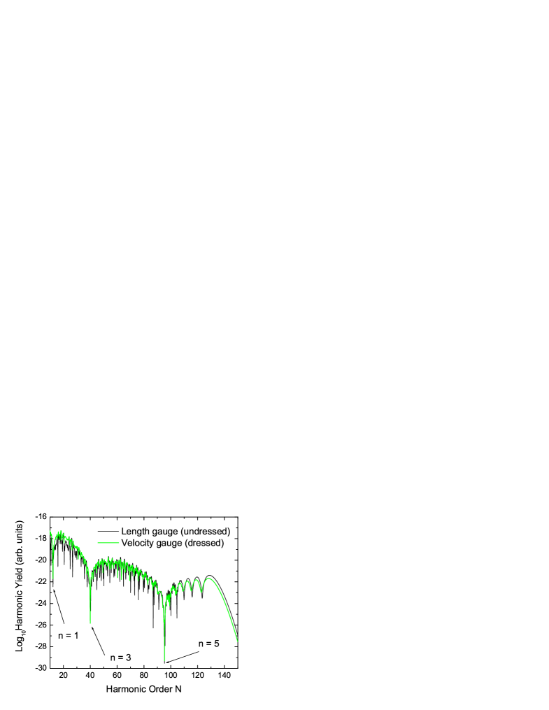
In Fig. 8, we display high-order harmonic spectra for the field-dressed SFA in the length gauge, and for the field-undressed SFA in the velocity gauge [panels (a) and (b), respectively]. For simplicity, we exhibit the results obtained with the modified prefactor (20), instead of a modified action. We also provide curves for which only the cosine term has been set to one, in order to facilitate the identification of interference effects. As an overall feature, we do not observe the interference patterns exhibited in the previous figures. Indeed, the curves with and without the cosine term are very similar. There is, however, a minimum near $\Omega=115\omega$ for the former case.

For the dressed length-gauge SFA, the above-stated features can be attributed to the fact that the condition for maxima and minima is now given by (17), with $\mathbf{p}$ instead of $\mathbf{\tilde{p}}=\mathbf{p}+\mathbf{A}(t).$ The harmonic frequencies for which they occur can be easily obtained from condition (6), and are given by

An upper bound for $\Omega$ can be estimated as follows. At the electron return times, the vector potential is roughly $A(t)\lesssim 2\sqrt{U_{p}}.$ This yields, for the parameters in Fig. 8, $\Omega\sim 121\omega$, which is slightly larger than the minimum encountered.

A breakdown of the interference patterns also occurs in the velocity gauge, for the very same reasons. Indeed, the interference condition for the SFA in the velocity gauge and for the field-dressed SFA in the length gauge are identical. This is a direct consequence of the fact that field-free initial and final electron states in the velocity gauge are gauge-equivalent to the field-dressed states considered in this paper. This gauge equivalence will lead to identical recombination form factors $d_{\mathrm{rec}}(\mathbf{p})=\left\langle\mathbf{p}\right|\mathcal{O}_{\mathrm{dip}}.\mathbf{e}_{x}\left|\psi_{0}\right\rangle$. Since the interference conditions (17) are mainly determined by $d_{\mathrm{rec}}(\mathbf{p})$, they will be the same. Hence, the harmonic orders for which the maxima and minima occur are given by Eq. (38), and therefore are unrealistically high. The discrepancies between both yields stem from the form factors $d_{\mathrm{ion}}(\mathbf{p})=\left\langle\mathbf{p}\right|H_{\mathrm{int}}\mathbf{(}t^{\prime}\mathbf{)}\left|\psi_{0}\right\rangle$, which are gauge-dependent.

One may, however, consider field-dressed states in the velocity gauge, which are gauge-equivalent to field-free states in the length gauge. This is achieved by applying the transformation $\chi_{v\leftarrow l}=\exp[i\mathbf{A}(t)\cdot\mathbf{r}]$ in the initial and final length-gauge electronic bound states. This leads to a shift $\mathbf{p\rightarrow p+A}(t)$ on a momentum eigenstate $\left|\mathbf{p}\right\rangle$, which is exactly the opposite shift induced in the field-dressed length-gauge SFA. This shift has the main consequence that the interference condition (17) now holds for $\mathbf{\tilde{p}}=\mathbf{p}+\mathbf{A}(t)$, even in the velocity gauge. The results obtained employing such dressed states in the velocity-gauge SFA, depicted in Fig. 9, are indeed very similar to those obtained using its field undressed, length gauge formulation. In fact, we have observed mainly quantitative differences, due to different prefactors $d_{\mathrm{ion}}(\mathbf{\tilde{p}})$ footndion2 .

One should note, however, that the transformation $\chi_{v\leftarrow l}$ introduces the same additional potential energy shifts in the modified action as in the undressed length-gauge case. Thus, the price one pays for recovering the correct interference conditions is the loss of a direct connection to simple classical models.