High-Order Algorithms for Compressible Reacting Flow with Complex Chemistry
Abstract
In this paper we describe a numerical algorithm for integrating the multicomponent,
reacting, compressible Navier-Stokes equations, targeted for direct numerical
simulation of combustion phenomena. The algorithm addresses two shortcomings
of previous methods. First, it incorporates an eighth-order
narrow stencil approximation of diffusive terms that reduces the communication compared
to existing methods and removes the need to use a filtering algorithm to remove
Nyquist frequency oscillations that are not damped with traditional approaches. The
methodology also incorporates a multirate temporal integration strategy that provides
an efficient mechanism for treating chemical mechanisms that are stiff relative to fluid
dynamical time scales. The overall methodology is eighth order in space with options for fourth order to eighth order in time.
The implementation uses a hybrid programming model designed for effective utilization of
many-core architectures.
We present numerical results demonstrating the convergence properties of the algorithm
with realistic chemical kinetics
and illustrating its performance characteristics.
We also present a validation example showing that the algorithm matches detailed results
obtained with an established low Mach number solver.
keywords:
DNS; spectral deferred corrections; finite difference; high-order methods; flame simulations1 Introduction
The simulation of a turbulent reacting flow without the use of either turbulence models or closure models for turbulence chemistry interaction is referred to as a direct numerical simulation, or DNS. One of the standard computational tools used in DNS studies of combustion is the numerical integration of the multicomponent, reacting compressible Navier-Stokes equations. DNS approaches have been in active use in the combustion community for more than twenty-five years; a comprehensive review of the literature is outside the scope of this article. Examples of early work in the field can be found in [3, 15, 28, 38, 17, 8]. With the advent of massively parallel, high performance computer architectures, it is now feasible to perform fully compressible DNS simulations for turbulent flows with detailed kinetics. See, for example, [35, 31, 40, 21].
Compressible DNS approaches place a premium on high order of accuracy. Spatial discretizations are typically based on defining high-order spatial derivative operators, , and . Common choices are central difference approximations [19] or compact differences based on Pade approximations [23]. Two codes that have seen significant application in combustion, SENGA [17, 7] and S3D [32, 40, 21], use tenth and eighth order central differences, respectively. Second-order derivative terms are approximated using repeated application of the first-order derivative operators, namely
This treatment of second-order derivatives does not provide adequate damping for Nyquist-frequency oscillations. Consequently some type of higher-order filter is employed periodically to damp high-frequency components of the system. Alternatively, the chain rule can be applied to second-order derivative terms. However, the chain rule approach is known to have stability issues (see e.g., [18]). Discretization of the spatial operators results in a system of ordinary differential equations (ODEs), which are typically integrated using high-order explicit Runge Kutta schemes such as those discussed by Kennedy et al. [20].
Although these types of compressible DNS codes have been highly successful, they suffer from two basic weaknesses. First, the use of explicit integration techniques limits the time step to the minimum of acoustic and chemical time scales. (Diffusive time scales are typically less restrictive than acoustic time scales for DNS.) This can be particularly restrictive for detailed chemical kinetics that can be stiff on acoustic time scales. The time step restriction can be relaxed by using an implicit / explicit temporal integration scheme such as IMEX but at the expense of solving linear systems to implicitly advance the kinetics at acoustic time scales.
The other issue with traditional compressible DNS methodology is the evaluation of second-order derivative terms by repeated application of the high-order first derivative operators. This approach is efficient in terms of floating point work but requires either multiple communication steps or much wider layers of ghost cells for each evaluation of the spatial operators. Although this type of design has been effective, as we move toward new many-core architectures that place a premium on reduced communication, the algorithm becomes communication bound and computational efficiency is reduced.
In this paper, we introduce two new algorithmic features that address the weaknesses discussed above. For the spatial discretization, we introduce an extension of the sixth-order narrow stencil finite difference algorithm of Kamakoti and Pantano [18] that provides a single discretization of to eighth-order accuracy. This approach requires significantly more floating point work than the standard approach but allows the spatial discretization to be computed with less communication. Furthermore, it eliminates the need for a filter to damp Nyquist-frequency oscillations. We also introduce a multirate time stepping strategy based on spectral deferred corrections (SDC) that enables the chemistry to be advanced on a different time scale than the fluid dynamics. This allows the fluid dynamics to be evaluated less frequently than in a fully coupled code resulting in shorter run times. These algorithms are implemented in a hybrid OpenMP/MPI parallel code named SMC.
In §2 we introduce the spatial discretization used by SMC and the eighth-order narrow stencil discretization of variable coefficient diffusion operators. In §3 we discuss the temporal discretization used by SMC and the multirate spectral deferred correction algorithm. In §4 we discuss some of the issues associated with a hybrid parallel implementation of SMC. In particular, we discuss a spatial blocking strategy that provides effective use of OpenMP threads. In §5 we present numerical results illustrating the convergence properties and parallel performance of SMC, and show its application to dimethyl ether-air combustion. Finally, the main results of the paper are summarized in §6.
2 Spatial Discretization
2.1 Navier-Stokes Equations
The multicomponent reacting compressible Navier-Stokes equations are given by
| (1a) | ||||
| (1b) | ||||
| (1c) | ||||
| (1d) | ||||
where is the density, is the velocity, is the pressure, is the specific energy density (kinetic energy plus internal energy), is the temperature, is the viscous stress tensor, and is the thermal conductivity. For each of the chemical species , is the mass fraction, is the diffusive flux, is the specific enthalpy, and is the production rate. The system is closed by an equation of state that specifies as a function of , and . For the examples presented here, we assume an ideal gas mixture.
The viscous stress tensor is given by
| (2) |
where is the shear viscosity and is the bulk viscosity.
A mixture model for species diffusion is employed in SMC. We define an initial approximation to the species diffusion flux given by
| (3) |
where is the mole fraction, and is the diffusion coefficient of species . For species transport to be consistent with conservation of mass we require
| (4) |
In general, the fluxes defined by (3) do not satisfy this requirement and some type of correction is required. When there is a good choice for a reference species that has a high molar concentration throughout the entire domain, one can use (3) to define the species diffusion flux (i.e., ) for all species except the reference, and then use (4) to define the flux of the reference species. This strategy is often used in combustion using as the reference species. An alternative approach [30] is to define a correction velocity given by
| (5) |
and then to set
| (6) |
The SMC code supports both of these operating modes. We will discuss these approaches further in §2.4.
2.2 Eighth-Order and Sixth-Order Discretization
The SMC code discretizes the governing Navier-Stokes equations (1) in space using high-order centered finite-difference methods. For first order derivatives a standard order stencil is employed. For second order derivatives with variable coefficients of the form
| (7) |
a novel order narrow stencil is employed. This stencil is an extension of those developed by Kamakoti and Pantano [18]. The derivatives in (7) on a uniform grid are approximated by
| (8) |
where
| (9) |
, and is an matrix (in general, for a discretization of order , is a matrix). This discretization is conservative because (8) is in flux form. Note, however, that is not a high-order approximation of the flux at even though the flux difference (8) approximates the derivative of the flux to order . This type of stencil is narrow because the width of the stencil is only for both and . In contrast, the width of a wide stencil in which the first-order derivative operator is applied twice is for and for .
Following the strategy in [18], a family of order narrow stencils for the second order derivative in (7) has been derived. The resulting order stencil matrix is given by
| (10) |
where
and and are two free parameters. Note that the well-posedness requirement established in [18] is satisfied by the stencil matrix above independent of the two free parameters. In SMC the default values of the free parameters were set to and to minimize an upper bound on truncation error that is calculated by summing the absolute value of each term in the truncation error. Additional analysis of truncation errors and numerical experiments on the order narrow stencil using various choices of the two parameters are presented in Appendix 7.
The SMC code uses a order stencil near physical boundaries where the conditions outside the domain are not well specified (see §2.5). The general order stencil matrix is given by
| (11) |
where
and is a free parameter. The order narrow stencil developed in [18] is a special case of the general order stencil when . Like the order stencil, the well-posedness and the order of accuracy for the order stencil is independent of the free parameter. In SMC, the free parameter is set to to minimize an upper bound on truncation error that is calculated by summing the absolute value of each term in the truncation error.
2.3 Cost Analysis of Eighth-Order Stencil
The order narrow stencil presented in § 2.2 requires significantly more floating-point operations (FLOPs) than the standard wide stencil, but has the benefit of less communication. The computational cost of a single evaluation the narrow stencil, for cells in one dimension, is FLOPs (this is the cost of operations in (9) and (8), excluding the division by ). For the order wide stencil with two steps of communication, the computational cost on cells is FLOPs. Hence, the narrow stencil costs more FLOPs than the wide stencil on cells in one dimension. As for communication, the wide stencil requires more bytes than the narrow stencil for cells with 8 ghost cells in one dimension. Here we assume that an 8-byte double-precision floating-point format is used. Ignoring latency, the difference in time for the two algorithms is then
where is the floating-point operations per second (FLOPS) and is the network bandwidth. To estimate this difference on current machines, we used the National Energy Research Scientific Computing Center’s newest supercomputer Edison as a reference. Each compute node on Edison has a peak performance of 460.8 GFLOPs (Giga-FLOPs per second), and the MPI bandwidth is about 8 GB/s 111The configuration of Edison is available at http://www.nersc.gov/users/computational-systems/edison/configuration/.. For in one dimension, the run time cost for the extra FLOPs of the narrow stencil is about , which is about 1.6 times of the extra communication cost of the wide stencil, . It should be emphasized that the estimates here are crude for several reasons. We neglected the efficiency of both floating-point and network operations for simplicity. In counting FLOPs, we did not consider a fused multiply-add instruction or memory bandwidth. In estimating communication costs, we did not consider network latency, the cost of data movement if MPI messages are aggregated to reduce latency, or communication hiding through overlapping communication and computation. Moreover, the efficiency of network operations is likely to drop when the number of nodes used increases, whereas the efficiency of FLOPs alone is independent of the number of total nodes. Nevertheless, as multicore systems continue to evolve, the ratio of FLOPS to network bandwidth is most likely to increase. Thus, we expect that the narrow stencil will cost less than the wide stencil on future systems, although any net benefit will depend on the systems configuration. As a data point, we note that both stencils are implemented in SMC, and for a test with cells using 512 MPI ranks and 12 threads on 6144 cores of Edison, a run using the narrow stencil took about the same time as using the wide stencil. Further measurements are presented in §5.2.
2.4 Correction for Species Diffusion
In §2.1, we introduced the two approaches employed in SMC to enforce the consistency of the mixture model of species diffusion with respect to mass conservation. The first approach uses a reference species and is straightforward to implement. We note that the last term in (1d) can be treated as , where is the species enthalpy for the reference species, because of (4). The second approach uses a correction velocity (5) and involves the computation of and . Although one might attempt to compute the correction velocity according to , where for species is computed using (9), this would reduce the accuracy for correction velocity to second-order since is only a second-order approximation to the flux at . To maintain order accuracy without incurring extra communication and too much extra computation, we employ the chain rule for the correction terms. For example, we compute as , and use , where is computed using the order narrow stencil for second order derivatives. The velocity correction form arises naturally in multicomponent transport theory; namely, it represents the first term in an expansion of the full multicomponent diffusion matrix. (See Giovangigli [13].) For that reason, velocity correction is the preferred option in SMC.
2.5 Physical Boundaries
The SMC code uses characteristic boundary conditions to treat physical boundaries. Previous studies in the literature have shown that characteristic boundary conditions can successfully lower acoustic reflections at open boundaries without suffering from numerical instabilities. Thompson [36, 37] applied the one-dimensional approximation of the characteristic boundary conditions to the hyperbolic Euler equations, and the one-dimensional formulation was extended by Poinsot and Lele [29] to the viscous Navier-Stokes equations. For multicomponent reacting flows, Sutherland and Kennedy [34] further improved the treatment of boundary conditions by the inclusion of reactive source terms in the formulation. In SMC, we have adopted the formulation of characteristic boundary conditions proposed in [41, 39], in which multi-dimensional effects are also included.
The order stencils used in SMC require four cells on each side of the point where the derivative is being calculated. Near the physical boundaries where the conditions outside the domain are unknown, lower order stencils are used for derivatives with respect to the normal direction. At the fourth and third cells from the boundary we use and order centered stencils respectively, for both advection and diffusion. At cells next to the boundary we reduce to centered second-order for diffusion and a biased third-order discretization for advection. Finally, for the boundary cells, a completely biased second-order stencil is used for diffusion and a completely biased third-order stencil is used for advection.
3 Temporal Discretization
3.1 Spectral Deferred Corrections
SDC methods for ODEs were first introduced in [10] and have been subsequently refined and extended in [25, 26, 16, 14, 5, 22]. SDC methods construct high-order solutions within one time step by iteratively approximating a series of correction equations at collocation nodes using low-order sub-stepping methods.
Consider the generic ODE initial value problem
| (12) |
where ; ; and . SDC methods are derived by considering the equivalent Picard integral form of (12) given by
| (13) |
A single time step is divided into a set of intermediate sub-steps by defining collocation points such that . Then, the integrals of over each of the intervals are approximated by
| (14) |
where , , and are quadrature weights. The quadrature weights that give the highest order of accuracy given the collocation points are obtained by computing exact integrals of the Lagrange interpolating polynomial over the collocation points . Note that each of the integral approximations (that represent the integral of from to ) in (14) depends on the function values at all of the collocation nodes .
To simplify notation, we define the integration matrix to be the matrix consisting of entries ; and the vectors and . With these definitions, the Picard equation (13) within the time step is approximated by
| (15) |
where . Note again that the integration matrix is dense so that each entry of depends on all other entries of (through ) and . Thus, (15) is an implicit equation for the unknowns in at all of the quadrature points. Finally, we note that the solution of (15) corresponds to the collocation or implicit Runge-Kutta solution of (12) over the nodes . Hence SDC can be considered as an iterative method for solving the spectral collocation formulation.
The SDC scheme used here begins by spreading the initial condition to each of the collocation nodes so that the provisional solution is given by . Subsequent iterations (denoted by superscripts) proceed by applying the node-to-node integration matrix to and correcting the result using a forward-Euler time-stepper between the collocation nodes. The node-to-node integration matrix is used to approximate the integrals (as opposed to the integration matrix which approximates ) and is constructed in a manner similar to the integration matrix . The update equation corresponding to the forward-Euler sub-stepping method for computing is given by
| (16) |
where is the row of . The process of computing (16) at all of the collocation nodes is referred to as an SDC sweep or an SDC iteration. The accuracy of the solution generated after SDC iterations done with such a first-order method is formally as long as the spectral integration rule (which is determined by the choice of collocation nodes ) is at least order .
Here, a method of lines discretization based on the spatial discretization presented in §2 is used to reduce the partial differential equations (PDEs) in question to a large system of ODEs.
The computational cost of the SDC scheme used here is determined by the number of nodes chosen and the number of SDC iterations taken per time step. The number of resulting function evaluations is . For example, with 3 Gauss-Lobatto () nodes, the resulting integration rule is order. To achieve this formal order of accuracy we perform SDC iterations per time step and hence we require function evaluations (note that is recycled from the previous time step, and hence the first time-step requires 9 function evaluations).
By increasing the number of SDC nodes and adjusting the number of SDC iterations taken, we can construct schemes of arbitrary order. For example, to construct a order scheme one could use a 5 point Gauss-Lobatto integration rule (which is order accurate), but only take 6 SDC iterations. For high order explicit schemes used here we have observed that the SDC iterations sometimes converge to the collocation solution in fewer iterations than is formally required. This can be detected by computing the SDC residual
| (17) |
where is the last row of , and comparing successive residuals. If is close to one, the SDC iterations have converged to the collocation solution and subsequent iterations can be skipped.
3.2 Multirate Integration
Multirate SDC (MRSDC) methods use a hierarchy of SDC schemes to integrate systems that contain processes with disparate time-scales more efficiently than fully coupled methods [5, 22]. A traditional MRSDC method integrates processes with long time-scales with fewer SDC nodes than those with short time-scales. They are similar in spirit to sub-cycling schemes in which processes with short characteristic time-scales are integrated with smaller time steps than those with long characteristic time-scales. MRSDC schemes, however, update the short time-scale components of the solutions at the long time-scale time steps during each MRSDC iteration, as opposed to only once for typical sub-cycling schemes, which results in tighter coupling between processes throughout each time-step [5, 22]. The MRSDC schemes presented here generalize the structure and coupling of the quadrature node hierarchy relative to the schemes first presented in [5, 22].
Before presenting MRSDC in detail, we note that the primary advantage of MRSDC schemes lies in how the processes are coupled. For systems in which the short time-scale process is moderately stiff, using more SDC nodes than the long time-scale process helps alleviate the stiffness of the short time-scale processes. However, extremely stiff processes are best integrated between SDC nodes with, for example, a variable order/step-size backward differentiation formula (BDF) scheme. In this case, the short time-scale processes can in fact be treated with fewer SDC nodes than long time-scale processes.
Consider the generic ODE initial value problem with two disparate time-scales
| (18) |
where we have split the generic right-hand-side in (12) into two components: and . A single time step is first divided into a set of intermediate sub-steps by defining collocation points such that . The vector of these collocation points is denoted , and these collocation points will be used to integrate the component. The time step is further divided by defining collocation points such that , where is the vector of these new collocation points. These collocation points will be used to integrate the component. That is, a hierarchy of collocation points is created with . The splitting of the right-hand-side in (18) should be informed by the numerics at hand. Traditionally, slow time-scale processes are split into and placed on the nodes, and fast time-scale processes are split into and places on the nodes. However, if the fast time-scale processes in the MRSDC update equation (20) are extremely stiff then it is more computationally effective to advance these processes using stiff integration algorithms over a longer time scale. In this case, we can swap the role of of the processes within MRSDC and treat the explicit update on the faster time scale (i.e., with the nodes). As such, we hereafter refer to the collocation points in as the “coarse nodes” and those in as the “fine nodes”.
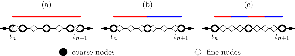
The SDC nodes for the coarse component are typically chosen to correspond to a formal quadrature rule like the Gauss-Lobatto rule. These nodes determine the overall order of accuracy of the resulting MRSDC scheme. Subsequently, there is some flexibility in how the nodes for fine components are chosen. For example, the points in can be chosen to correspond to a formal quadrature rule
-
(a)
over the entire time step ;
-
(b)
over each of the intervals defined by the points in ;
-
(c)
over several sub-intervals of the intervals defined by the points in ;
Note that in the first case, a quadrature rule that nests (or embeds) itself naturally is required (such as the Clenshaw-Curtis rule), whereas in the second and third cases the nodes in usually do not correspond to a formal quadrature rule over the entire time step . In the second and third cases we note that the basis used to construct the and integration matrices are typically piecewise polynomial – this allows us to shrink the effective time-step size of the fine process without constructing an excessively high-order polynomial interpolant. These three possibilities are depicted in Fig. 1.
Once the SDC nodes for the desired MRSDC scheme have been chosen, the node-to-node and regular integration matrices ( and , respectively) can be constructed. While single-rate SDC schemes, as presented in §3.1, require one set of and matrices, the two-component MRSDC scheme used here requires two sets of and matrices. These are denoted with subscripts so that the action of approximates the node-to-node integrals between nodes in of the component that “lives” on the nodes, and similarly for the matrices. Note that both and are of size .
With these definitions, the Picard equation (13) within the time step is approximated by
| (19) |
where is the vector of approximate solution values over the fine nodes in . The MRSDC scheme used in SMC has two operating modes:
- 1.
- 2.
In the first mode, the scheme is purely explicit whereas in the second mode the algorithm uses an implicit treatment of reactions. Which version is most appropriate for a given simulation depends on the relative stiffness of chemistry and fluid dynamics. When the chemical time scales are not significantly disparate from the fluid mechanical time scale, the fully explicit version will be the most efficient. When the chemistry is extremely stiff, the second mode is preferred.
The MRSDC update equation used in SMC for mode 1 over the nodes in is given by
| (20) | ||||
where is the row of , and the node of the fine component corresponds to the closest coarse node to the left of the fine node . That is, the coarse component is held constant, and equal to its value at the left coarse node , during the fine updating steps. The update equation for mode 2 is
| (21) | ||||
where is computed with VODE.
The computational cost of an MRSDC scheme is determined by the number of nodes chosen for each multirate component and the number of SDC iterations taken per time step. The number of resulting function evaluations per component is . For example, with 3 Gauss-Lobatto () nodes for the coarse component and 5 Gauss-Lobatto nodes for the fine component between each of the coarse nodes (so that there are 9 nodes in and hence ), the number of coarse function evaluations over iterations is , and the number of fine function evaluations is .
The reacting compressible Navier-Stokes equations (1) have two characteristic time-scales: one over which advection and diffusion processes evolve, and another over which reactions evolve. The reaction time-scale is usually shorter than the advection/diffusion time-scale. As such, the coarse and fine MRSDC nodes typically correspond to the advection/diffusion and reaction parts of (1), respectively. However, as is the case for the Dimethyl Ether Jet problem shown in §5.3, the reaction terms in (1) can become so stiff that it becomes impractical to integrate them explicitly. In these cases, SMC employs the variable-order BDF schemes in VODE [6] to integrate the reaction terms implicitly. This effectively reverses the time-step constraint of the system: the reaction terms can be integrated using VODE (which internally takes many steps) with a larger time-step than the advection-diffusion terms. As such, the roles of the coarse and fine MRSDC nodes can be reversed so that the coarse and fine MRSDC nodes correspond to the reaction and advection-diffusion terms of (1), respectively, thereby amortizing the cost of the implicit solves by using fewer SDC nodes to integrate the stiff chemistry.
4 Parallelization
SMC is implemented within the BoxLib software framework with a hybrid MPI-OpenMP approach for parallelization [1]. In BoxLib, the computational domain is divided into boxes. Each MPI process owns one or more boxes via decomposition of the spatial domain and it can spawn multiple OpenMP threads. For parallelization with OpenMP, the traditional approach is a fine-grained approach in which individual loops are threaded using OpenMP PARALLEL DO directives (with COLLAPSE clause if the number of threads is relatively large). This approach works well for tasks like computing transport coefficients and chemistry production rates because there is only one PARALLEL DO region for each box. However, this approach to fine-grained parallelism does not work well for computing diffusive and hyperbolic terms. The reason for this is that many loops are used in computing terms like . This results in many PARALLEL DO regions with serial parts in between that, in turn, can incur significant overheads and limit parallel efficiency. To overcome these issues in the fine-grained parallelism approach, a coarser-grained approach is taken for computing diffusive and hyperbolic terms. In this approach, OpenMP PARALLEL DO directives are not used. Instead, a SPMD (single program, multiple data) style is used. Each thread works on its own domain. Listing 1 shows a code snippet illustrating the coarse-grained parallelism approach. Here q, D and dUdt are four-dimensional Fortran arrays for primitive variables, transport coefficients, and rate of change of conserved variables, respectively. These shared arrays contain data for the entire box. The get_threadbox subroutine computes the bounds of sub-boxes owned by each thread and stores them in private arrays lo and hi. The original box (without ghost cells) is entirely covered by the sub-boxes without overlap. Typically, the domain decomposition among threads is performed in and -dimensions, but not in -dimension, because the -dimension of our data arrays is contiguous in memory. The diffterm subroutine is called by each thread with private lo and hi, and it has local variables (including arrays) that are automatically private to each thread. Note that there are no OpenMP statements in the diffterm subroutine. This approach reduces synchronization points and thread overhead, resulting in improved thread scaling as demonstrated in the next section.
5 Numerical Results
In this section we present numerical tests to demonstrate the theoretical rate of convergence and performance of SMC. We also compare simulation results obtained using SMC with the results from the low Mach number LMC code [9, 4, 27]. Numerical simulations presented here use EGLIB [12, 11] to compute transport coefficients.
5.1 Convergence
5.1.1 Space/time Convergence
In this section we present numerical tests to demonstrate the theoretical rate of convergence of SMC for the single-rate SDC integrator.
The convergence tests presented here are set up as follows. The simulations use a 9-species reaction mechanism [24]. The computational domain is with periodic boundaries in all three dimensions. The initial pressure, temperature and velocity of the gas are set to
| (22) | ||||
| (23) | ||||
| (24) | ||||
| (25) | ||||
| (26) |
where , , , , , and . The mole fractions of species are initially set to zero except that
| (27) | ||||
| (28) | ||||
| (29) |
To demonstrate convergence, we performed a series of runs with increasing spatial and temporal resolutions. A single-rate SDC scheme with 5 Gauss-Lobatto nodes and 8 SDC iterations is used for time stepping. The simulations are stopped at . When the spatial resolution changes by a factor of 2 from one run to another, we also change the time step by a factor of 2. Therefore, the convergence rate in this study is expected to be order. Table 5.1.1 shows the and -norm errors and convergence rates for , , , , , , , and . Because there is no analytic solution for this problem, we compute the errors by comparing the numerical solution using points with the solution using points. The -norm error is computed as
| (30) |
where is the solution at point of the point run and is the solution of the point run at the same location. The results of our simulations demonstrate the high-order convergence rate of our scheme. The and -norm convergence rates for various variables in the simulations approach order, the theoretical order of the scheme. Relatively low orders are observed at low resolution because the numerical solutions are not in the regime of asymptotic convergence yet.
Errors and convergence rates for three-dimensional simulations
of a hydrogen flame using single-rate SDC and 8th order
finite difference stencil. Density , temperature and
are in SI units.
Variable
No. of Points
Error
Rate
Error
Rate
4
2.613E-08
5.365E-09
2
3.354E-10
6.28
6.655E-11
6.33
1
2.053E-12
7.35
3.438E-13
7.60
0.5
8.817E-15
7.86
1.437E-15
7.90
4
3.328E-02
6.722E-03
2
4.184E-04
6.31
8.266E-05
6.35
1
2.515E-06
7.38
4.266E-07
7.60
0.5
1.095E-08
7.84
1.783E-09
7.90
4
6.184E+00
8.451E-01
2
7.368E-02
6.39
8.859E-03
6.58
1
4.554E-04
7.34
4.559E-05
7.60
0.5
2.011E-06
7.82
1.904E-07
7.90
4
6.677E+00
8.801E-01
2
7.218E-02
6.53
9.121E-03
6.59
1
4.784E-04
7.24
4.693E-05
7.60
0.5
2.041E-06
7.87
1.961E-07
7.90
4
6.443E+00
8.632E-01
2
7.211E-02
6.48
8.987E-03
6.59
1
4.626E-04
7.28
4.624E-05
7.60
0.5
2.034E-06
7.83
1.932E-07
7.90
4
5.507E-08
1.272E-08
2
8.619E-10
6.00
1.764E-10
6.17
1
5.802E-12
7.21
9.828E-13
7.49
0.5
2.512E-14
7.85
4.169E-15
7.88
4
1.358E-06
9.166E-08
2
1.406E-08
6.59
7.136E-10
7.00
1
7.111E-11
7.63
3.468E-12
7.68
0.5
2.982E-13
7.90
1.433E-14
7.92
4
3.858E-12
3.791E-14
2
2.740E-14
7.14
2.661E-16
7.15
1
1.288E-16
7.73
1.245E-18
7.74
0.5
5.278E-19
7.93
5.093E-21
7.93
4
7.994E-12
7.318E-14
2
5.847E-14
7.09
5.347E-16
7.10
1
2.778E-16
7.72
2.548E-18
7.71
0.5
1.141E-18
7.93
1.048E-20
7.93
4
1.328E-06
8.762E-08
2
1.383E-08
6.58
6.622E-10
7.05
1
6.999E-11
7.63
3.160E-12
7.71
0.5
2.943E-13
7.89
1.300E-14
7.92
5.1.2 Multirate Integration
In this section we present numerical tests to demonstrate the theoretical convergence rate of the MRSDC integrator in SMC.
Table 5.1.2 shows the and -norm errors and convergence rates for , , , , , , , and for the same test problem as described in §5.1, except that and . All runs were performed on a grid, so that the errors and convergence rates reported here are ODE errors. Because there is no analytic solution for this problem, a reference solution was computed using the same spatial grid, but with an -order single-rate SDC integrator and s. We note that the and -norm convergence rates for all variables and MRSDC configurations are -order, as expected since the coarse MRSDC component uses 3 Gauss-Lobatto nodes. This verifies that the MRSDC implementation in SMC operates according to its specifications regardless of how the fine nodes are chosen (see §3.2).
Errors and convergence rates for three-dimensional simulations
of a hydrogen flame using 4th order MRSDC and 8th order
finite difference stencil. Density , temperature and
are in SI units.
The MRSDC / configurations use coarse nodes and fine nodes between each pair of coarse nodes (type (b) in §3.2).
The MRSDC / configurations use coarse nodes
and fine nodes repeated times between each pair of coarse
nodes (type (c) in §3.2). All SDC nodes are
Gauss-Lobatto (GL) nodes. Density , temperature and
are in SI units.
SDC Configuration
Variable
Error
Rate
Error
Rate
GL 3 / GL 9
10
5.638e-07
3.958e-08
5
3.392e-08
4.06
2.426e-09
4.03
2.5
2.093e-09
4.02
1.509e-10
4.01
10
2.748e-04
1.577e-05
5
1.661e-05
4.05
9.504e-07
4.05
2.5
1.029e-06
4.01
5.877e-08
4.02
10
6.928e-04
2.253e-05
5
4.255e-05
4.03
1.369e-06
4.04
2.5
2.650e-06
4.01
8.496e-08
4.01
10
1.960e-09
5.051e-11
5
1.160e-10
4.08
3.059e-12
4.05
2.5
7.108e-12
4.03
1.896e-13
4.01
10
9.501e-09
3.340e-10
5
5.762e-10
4.04
2.027e-11
4.04
2.5
3.562e-11
4.02
1.255e-12
4.01
10
5.989e-17
3.531e-19
5
3.671e-18
4.03
2.183e-20
4.02
2.5
2.292e-19
4.00
1.370e-21
3.99
10
4.309e-18
6.660e-20
5
2.519e-19
4.10
3.928e-21
4.08
2.5
1.527e-20
4.04
2.394e-22
4.04
10
8.743e-09
3.191e-10
5
5.258e-10
4.06
1.938e-11
4.04
2.5
3.238e-11
4.02
1.200e-12
4.01
GL 3 / GL 5 2
10
5.638e-07
3.958e-08
5
3.392e-08
4.06
2.426e-09
4.03
2.5
2.093e-09
4.02
1.509e-10
4.01
10
2.748e-04
1.577e-05
5
1.661e-05
4.05
9.504e-07
4.05
2.5
1.029e-06
4.01
5.877e-08
4.02
10
6.928e-04
2.253e-05
5
4.255e-05
4.03
1.369e-06
4.04
2.5
2.650e-06
4.01
8.496e-08
4.01
10
1.960e-09
5.051e-11
5
1.160e-10
4.08
3.059e-12
4.05
2.5
7.108e-12
4.03
1.896e-13
4.01
10
9.501e-09
3.340e-10
5
5.762e-10
4.04
2.027e-11
4.04
2.5
3.562e-11
4.02
1.255e-12
4.01
10
5.989e-17
3.531e-19
5
3.671e-18
4.03
2.183e-20
4.02
2.5
2.292e-19
4.00
1.370e-21
3.99
10
4.309e-18
6.660e-20
5
2.519e-19
4.10
3.928e-21
4.08
2.5
1.527e-20
4.04
2.394e-22
4.04
10
8.743e-09
3.191e-10
5
5.258e-10
4.06
1.938e-11
4.04
2.5
3.238e-11
4.02
1.200e-12
4.01
5.2 Performance
5.2.1 Parallel Performance
In this section we present numerical tests to demonstrate the parallel efficiency of SMC.
Two strong scaling studies were performed: a pure OpenMP study on a 61-core Intel Xeon Phi, and a pure MPI study on the Hopper supercomputer at the National Energy Research Scientific Computing Center (NERSC).
The pure OpenMP strong scaling study was carried out on a 61-core 1.1 GHz Intel Xeon Phi coprocessor that supported up to 244 hyperthreads. We performed a series of pure OpenMP runs, each consisting of a single box of points, of the test problem in section 5.1 using various numbers of threads. The simulations are run for 10 time steps. Table 5.2.1 shows that SMC has excellent thread scaling behavior. An factor of 86 speedup over the 1 thread run is obtained on the 61-core coprocessor using 240 hyperthreads.
The pure MPI strong scaling study was carried out on the Hopper supercomputer at NERSC. Each compute node of Hopper has 4 non-uniform memory access (NUMA) nodes, with 6 cores on each NUMA node. We performed a series of pure MPI runs of the test problem in section 5.1 using various numbers of processors and integration schemes on a grid of points. The simulations are run for 10 time steps. Several observations can be made from the results listed in Table 5.2.1. First, when using a single processor the wide stencil is slightly faster than the narrow stencil regardless of the integration scheme used. This is consistent with the cost analysis of the stencils done in §2.3 which shows that the wide stencil uses fewer FLOPs per stencil evaluation than the narrow stencil. The difference in single-processor run times, however, is not significant which suggests that both stencils are operating in a regime dominated by memory access times. Second, when using multiple MPI processes, both the wall clock time per step and efficiency of the narrow stencil is consistently better than the wide stencil regardless of the integrator being used. Again, this is consistent with cost analysis done in §2.3 which shows that the communication cost associated with the narrow stencil is less than the wide stencil. The difference between the stencils when using multiple MPI processes is observable but not dramatic. Regarding parallel efficiency, we note that as more processors are used the amount of work performed grows due to the presence of ghost cells where, for example, diffusion coefficients need to be computed. As such, we cannot expect perfect parallel efficiency. In the extreme case were the problem is spread across 512 processors, each processor treats an box, which grows to a box with the addition of ghost cells. Finally, note that the parallel efficiency of the MRSDC scheme is higher than the SRSDC scheme regardless of the stencil being used since, for this test, the MRSDC scheme performs the same number of advection/diffusion evaluations (and hence stencil evaluations and extra ghost cell work) but performs significantly more evaluations of the chemistry terms – MRSDC has a higher arithmetic intensity with respect to MPI communications than SRSDC.
Strong scaling behavior of pure OpenMP runs on a 61-core Intel
Xeon Phi coprocessor. Average wall clock time per time step and speedup
are shown for runs using various number of threads. Hyperthreading
is used for the 128 and 240-thread runs.
No. of threads
Wall time per step (s)
Speedup
1
1223.58
2
626.13
2.0
4
328.97
3.7
8
159.88
7.7
16
79.73
16
32
40.12
31
60
24.55
50
128
18.19
67
240
14.28
86
Strong scaling behavior of pure MPI runs with grid points on the Hopper supercomputer at NERSC. Average wall clock time per time step, speedup, and efficiency
are shown for runs using various number of processors and schemes.
The SRSDC scheme uses single-rate SDC with 3 nodes, with narrow and wide stencils.
The MRSDC scheme uses multi-rate SDC with 3 fine nodes, and 5 fine nodes repeated 2 times between each coarse node (type (c) in §3.2). All SDC nodes are Gauss-Lobatto (GL) nodes.
Method/Stencil
No. of MPI processes
Wall time per step (s)
Speedup
Efficiency
SRSDC/Narrow
1
243.35
8
42.92
5.67
71%
64
7.91
30.84
48%
512
2.14
133.95
22%
SRSDC/Wide
1
231.60
8
43.21
5.36
67%
64
8.04
28.80
45%
512
2.27
102.09
20%
MRSDC/Narrow
1
695.57
8
101.86
6.82
85%
64
15.25
45.69
71%
512
3.15
220.55
43%
MRSDC/Wide
1
685.87
8
102.45
6.69
84%
64
15.75
43.55
68%
512
3.28
208.85
41%
We also performed a weak scaling study using the test problem in section 5.1 on the Hopper supercomputer at the NERSC. In this weak scaling study, a hybrid MPI/OpenMP approach with 6 threads per MPI process is used. Each MPI process works on two boxes. The simulations are run for 10 time steps. Table 5.2.1 shows the average wall clock time per time step for a series of runs on various numbers of cores. We use the 6-core run as baseline and define parallel efficiency for an -core run as , where and are the average wall clock time per time step for the 6 and -core runs, respectively. Excellent scaling to about 100 thousand cores is observed.
Weak scaling behavior of hybrid MPI/OpenMP runs on Hopper at NERSC. Average
wall clock time per time step and parallel efficiency are shown for
runs on various number of cores. Each MPI process spawns 6 OpenMP
threads.
No. of cores
No. of MPI processes
Wall time per step (s)
Efficiency
6
1
13.72
24
4
14.32
96%
192
32
14.46
95%
1536
256
14.47
95%
12288
2048
15.02
91%
98304
16384
15.32
90%
5.2.2 Multirate Integration
Table 5.2.2 compares run time and function evaluation counts for premixed methane flame using various configurations of SDC; MRSDC; and a six-stage, fourth-order Runge-Kutta integrator. The configuration is a cubic box (m) with periodic boundary conditions in the and directions, and inlet/outlet boundary conditions in the direction. The GRI-MECH 3.0 chemistry network (53 species, 325 reactions) [33] was used so that the reaction terms in (1) were quite stiff and an MRSDC integrator with the reaction terms on the fine nodes was appropriate. A reference solution was computed using a single-rate SDC integrator with a time step of s to a final time of s. All simulations were run on a point grid. For each integrator, the test was run using successively larger time steps until the solution no longer matched the reference solution. The largest time step that matched the reference solution (to within a relative error of less than ) is reported. All SDC integrators use 3 Gauss-Lobatto nodes for the coarse component and hence all integrators, including the Runge-Kutta integrators, are formally order accurate. We note that all of the multi-rate integrators are able to use larger time steps than the SRSDC and RK integrators due to the stiffness of the reaction terms: the multi-rate integrators use more nodes to integrate the reaction terms and hence the effective time-steps used in the update equation (20) are smaller. This means that, in all cases, the multi-rate integrators evaluate the advection/diffusion terms less frequently than the single-rate integrator. However, in all but one case, the multi-rate integrators also evaluate the reaction terms more frequently than the SRSDC and RK integrators. The trade-off between the frequency of evaluating the advection/diffusion vs reaction terms is highlighted by comparing the MRSDC 3 GL / 9 GL and MRSDC 3 GL / 13 GL runs: the run with 13 fine nodes can use a slightly larger time-step at the cost of evaluating the reaction terms more frequently, resulting in only a very slight runtime advantage over the run using 9 fine nodes and a smaller time-step. Ultimately the largest runtime advantage is realized by choosing a multi-rate configuration that allows a large time-step to be taken without requiring too many extra calls to the reaction network. For this test the MRSDC 3 / configuration achieves this goal and is able to run to completion approximately 6.0 times faster than the single-rate SDC integrator and 4.5 times faster than the RK integrator.
Comparison of runtime and function evaluation count for various configurations of SDC and MRSDC.
Function evaluation counts are reported as: no. of advection/diffusion evaluations / no. of chemistry evaluations.
All schemes use the narrow stencil, except where noted.
The SRSDC configuration uses single-rate SDC with nodes.
The RK scheme is fourth order and use six stages.
The MRSDC / configurations use MRSDC with coarse nodes and fine nodes between each pair of coarse nodes (type (b) in §3.2).
The MRSDC / configurations use MRSDC with coarse nodes and fine nodes repeated times between each pair of coarse nodes (type (c) in §3.2). All SDC nodes are Gauss-Lobatto (GL) nodes.
Scheme
(s)
Runtime (s)
Evaluations (AD/R)
SRSDC, 3 GL
6
130.6
561/561
RK, 6/4
6
96.5
420/420
RK, 6/4 wide
6
95.4
420/420
MRSDC, 3 GL / 9 GL type (b)
30
44.1
113/897
MRSDC, 3 GL / 13 GL type (b)
42
39.7
81/961
MRSDC, 3 GL / GL type (c)
60
30.8
57/897
MRSDC, 3 GL / GL type (c)
60
21.7
57/449
5.3 Dimethyl Ether Jet
We present here a two-dimensional simulation of jet using a 39-species dimethyl ether (DME) chemistry mechanism [2]. A 2D Cartesian domain, and , is used for this test. Pressure is initially set to everywhere. The initial temperature, velocity and mole fractions of species are set to
| (31) | ||||
| (32) | ||||
| (33) | ||||
| (34) |
where , , , and . The variable is given by
| (35) |
where and . The mole fractions of species for the “jet” and “air” states are set to zero except that
| (36) | ||||
| (37) | ||||
| (38) | ||||
| (39) |
An inflow boundary is used at the lower -boundary, whereas outflow boundary conditions are applied at the other three boundaries. Sinusoidal variation is added to the inflow velocity as follows,
| (40) |
where , is the length of the domain in -direction, and is the period of the variation. With these parameters, the resulting flow problem is in the low Mach number regime to facilitate cross-validation with an established low Mach number solver [9]
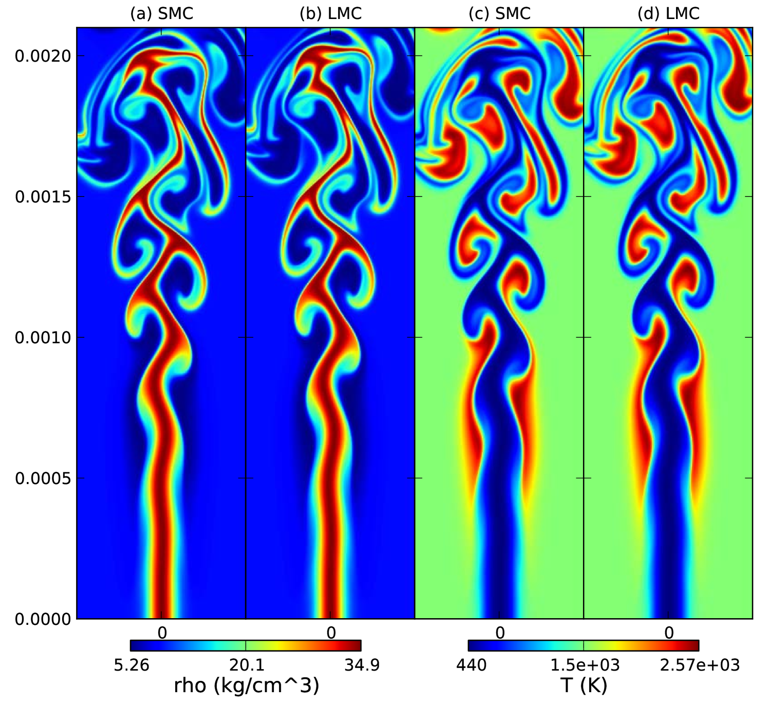
The 39-species DME mechanism used in this test is extremely stiff so that it becomes impractical to evolve the reaction system explicitly. Hence, we use the variable-order BDF scheme in VODE [6] for computing species production rates. In this test, we use MRSDC, and put the reaction terms in (1c) and advection-diffusion terms on the coarse and fine nodes, respectively. Due to the use of an implicit solver, we can evaluate the reaction terms on the coarse node with a large time step without suffering from instability. As for advection-diffusion terms, the time step is limited by the acoustic time scale. In this test, we use 5 coarse Gauss-Lobatto nodes for the reaction terms, whereas for the advection-diffusion terms we use 3 fine Gauss-Lobatto nodes repeated twice between each pair of coarse nodes. The time step is chosen to have a Courant-Friedrichs-Lewy (CFL) number of 2. The effective CFL numbers for a substep of advection-diffusion (i.e., the interval spanned by 3 fine Gauss-Lobatto nodes) are about 0.17 and 0.33. (Note that the 5 coarse Gauss-Lobatto nodes are not evenly distributed.) We perform 4 SDC iterations per time step. The simulation is run with uniform points corresponding to a cell size of up to time . The numerical results are shown in figures 2 & 3. As a validation of SMC, we have also presented the numerical results obtained using the LMC code that is based on a low-Mach number formulation [9, 4, 27] that approximates the compressible flow equation to . The results of the two codes are nearly indistinguishable in spite of the difference between the two formulations. This is because the maximum Mach number in this problem is only so the low Mach number model is applicable. We note that this simulation is essentially infeasible with a fully explicit solver because of the stiffness of the chemical mechanism.

6 Conclusions
We have described a numerical algorithm for integrating the multicomponent, reacting, compressible Navier-Stokes equations that is eight-order in space with fourth order to eighth order temporal integration. The methodology uses a narrow stencil approximation of diffusive terms that reduces the communication compared to existing methods and removes the need to use a filtering algorithm to remove Nyquist frequency oscillations that are not damped with traditional approaches. It also incorporates a multirate temporal integration strategy that provides an efficient mechanism for treating chemical mechanisms that are stiff relative to fluid dynamical time scales. The narrow stencil uses more floating point operations per stencil evaluation than the standard wide stencil but requires less communication. A strong scaling study demonstrated that the narrow stencil scales better than the wide stencil which has important ramifications for stencil performance on future multicore machines. The multirate integration approach supports two modes for operation. One treats the reactions explicitly using smaller time steps than are used for the fluid mechanics; the other treats reaction implicitly for case in which the chemical time scales are significantly faster than the fluid dynamical time scales. A performance study of the multi-rate integration scheme with realistic chemical kinetics showed that the multi-rate integrator can operate with a larger time-step compared to single-rate integrators and ultimately obtained an accurate solution in less time. The implementation uses a hybrid programming model designed for effective utilization of a large number of threads that is targeted toward next generation many-core architectures. The code scales well to approximately 100K cores and shows excellent thread performance on a 61-core Intel Xeon Phi coprocessor. We present numerical results demonstrating the convergence properties of the algorithm with realistic chemical kinetics and validating the algorithm against results obtained with an established low Mach number solver.
Acknowledgements
This work was supported by the Applied Mathematics Program and the Exascale Co-Design Program of the DOE Office of Advanced Scientific Computing Research under the U.S. Department of Energy under contract DE-AC02-05CH11231. This research used resources of the National Energy Research Scientific Computing Center, which is supported by the Office of Science of the U.S. Department of Energy under Contract No. DE-AC02-05CH11231.
References
- [1] Center for Computational Sciences and Engineering, Lawrence Berkeley National Laboratory, BoxLib, software available at https://ccse.lbl.gov/BoxLib/.
- [2] G. Bansal, A. Mascarenhas, J. H. Chen, T. Lu, and Z. Luo, Direct numerical simulations of autoignition in stratified dimethyl-ether (dme)/air turbulent mixtures, Combustion and Flame, in preparation (2013).
- [3] M. Baum, T. J. Poinsot, D. C. Haworth, and N. Darabiha, Direct numerical simulation of H2/O2/N2 flames with complex chemistry in two-dimensional turbulent flows, J. Fluid Mech., 281 (1994), pp. 1–32.
- [4] J. B. Bell, M. S. Day, A. S. Almgren, M. J. Lijewski, and C. A. Rendleman, Adaptive numerical simulation of turbulent premixed combustion, in Proceedings of the first MIT conference on computational fluid and solid mechanics, Cambridge, MA, June 2001, MIT Press.
- [5] A. Bourlioux, A. T. Layton, and M. L. Minion, High-order multi-implicit spectral deferred correction methods for problems of reactive flow, Journal of Computational Physics, 189 (2003), pp. 651–675.
- [6] P. Brown, G. Byrne, and A. Hindmarsh, Vode: A variable-coefficient ode solver, SIAM Journal on Scientific and Statistical Computing, 10 (1989), pp. 1038–1051.
- [7] N. Chakraborty and S. Cant, Unsteady effects of strain rate and curvature on turbulent premixed flames in an inflow-outflow configuration, Combustion and Flame, 137 (2004), pp. 129 – 147.
- [8] J. H. Chen and H. Im, Correlation of flame speed with stretch in turbulent premixed methane/air flames, Proc. Combust. Inst., 27 (1998), pp. 819–826.
- [9] M. S. Day and J. B. Bell, Numerical simulation of laminar reacting flows with complex chemistry, Combust. Theory Modelling, 4 (2000), pp. 535–556.
- [10] A. Dutt, L. Greengard, and V. Rokhlin, Spectral deferred correction methods for ordinary differential equations, BIT Numerical Mathematics, 40 (2000), pp. 241–266.
- [11] A. Ern, C. C. Douglas, and M. D. Smooke, Detailed chemistry modeling of laminar diffusion flames on parallel computers, Int. J. Sup. App., 9 (1995), pp. 167–186.
- [12] A. Ern and V. Giovangigli, Multicomponent Transport Algorithms, vol. m24 of Lecture Notes in Physics, Springer-Verlag, Berlin, 1994.
- [13] V. Giovangigli, Multicomponent Flow Modeling, Birkhäuser, Boston, 1999.
- [14] A. C. Hansen and J. Strain, Convergence theory for spectral deferred correction, Preprint, (2006).
- [15] D. C. Haworth and T. J. Poinsot, Numerical simulations of Lewis number effects in turbulent premixed flames, J. Fluid Mech., 244 (1992), pp. 405–436.
- [16] J. Huang, J. Jia, and M. Minion, Accelerating the convergence of spectral deferred correction methods, Journal of Computational Physics, 214 (2006), pp. 633–656.
- [17] K. Jenkins and R. Cant, Direct numerical simulation of turbulent flame kernels, in Recent Advances in DNS and LES, D. Knight and L. Sakell, eds., vol. 54 of Fluid Mechanics and its Applications, Springer Netherlands, 1999, pp. 191–202.
- [18] R. Kamakoti and C. Pantano, High-order narrow stencil finite-difference approximations of second-order derivatives involving variable coefficients, SIAM Journal on Scientific Computing, 31 (2010), pp. 4222–4243.
- [19] C. A. Kennedy and M. H. Carpenter, Several new numerical methods for compressible shear-layer simulations, Applied Numerical Mathematics, 14 (1994), pp. 397 – 433.
- [20] C. A. Kennedy, M. H. Carpenter, and R. M. Lewis, Low-storage, explicit runge-kutta schemes for the compressible navier-stokes equations, Applied Numerical Mathematics, 35 (2000), pp. 177 – 219.
- [21] H. Kolla, R. W. Grout, A. Gruber, and J. H. Chen, Mechanisms of flame stabilization and blowout in a reacting turbulent hydrogen jet in cross-flow, Combustion and Flame, 159 (2012), pp. 2755 – 2766. Special Issue on Turbulent Combustion.
- [22] A. T. Layton and M. L. Minion, Conservative multi-implicit spectral deferred correction methods for reacting gas dynamics, Journal of Computational Physics, 194 (2004), pp. 697–715.
- [23] S. K. Lele, Compact finite difference schemes with spectral-like resolution, Journal of Computational Physics, 103 (1992), pp. 16 – 42.
- [24] J. Li, Z. Zhao, A. Kazakov, and F. L. Dryer, An updated comprehensive kinetic model of hydrogen combustion, International Journal of Chemical Kinetics, 36 (2004), pp. 566–575.
- [25] M. L. Minion, Semi-implicit spectral deferred correction methods for ordinary differential equations, Communications in Mathematical Sciences, 1 (2003), pp. 471–500.
- [26] , Semi-implicit projection methods for incompressible flow based on spectral deferred corrections, Applied numerical mathematics, 48 (2004), pp. 369–387.
- [27] A. Nonaka, J. B. Bell, M. S. Day, C. Gilet, A. S. Almgren, and M. L. Minion, A deferred correction coupling strategy for low mach number flow with complex chemistry, Combustion Theory and Modelling, 16 (2012), pp. 1053–1088.
- [28] T. Poinsot, S. Candel, and A. Trouv , Applications of direct numerical simulation to premixed turbulent combustion, Progress in Energy and Combustion Science, 21 (1995), pp. 531 – 576.
- [29] T. Poinsot and S. Lelef, Boundary conditions for direct simulations of compressible viscous flows, Journal of Computational Physics, 101 (1992), pp. 104 – 129.
- [30] T. Poinsot and D. Veynante, Theoretical and Numerical Combustion, R. T. Edwards, Inc., Philadelphia, first ed., 2001.
- [31] R. Sankaran, E. R. Hawkes, J. H. Chen, T. Lu, and C. K. Law, Structure of a spatially developing turbulent lean methane-air bunsen flame, Proceedings of the Combustion Institute, 31 (2007), pp. 1291 – 1298.
- [32] R. Sankaran, E. R. Hawkes, C. Y. Yoo, J. H. Chen, T. Lu, and C. K. Law, Direct numerical simuation of stationary lean premixed methane-air flames under intense turbulence, in Proceedings of the 5th US Combustion Meeting (CD-ROM), Western States Section of the Combustion Institute, Mar. 2007. Paper B09.
- [33] G. P. Smith et al., GRI-Mech 3.0. Available at http://www.me.berkeley.edu/gri_mech.
- [34] J. C. Sutherland and C. A. Kennedy, Improved boundary conditions for viscous, reacting, compressible flows, Journal of Computational Physics, 191 (2003), pp. 502 – 524.
- [35] M. Tanahashi, M. Fujimura, and T. Miyauchi, Coherent fine scale eddies in turbulent premixed flames, Proc. Combust. Inst., 28 (2000), pp. 529–535.
- [36] K. W. Thompson, Time dependent boundary conditions for hyperbolic systems, Journal of Computational Physics, 68 (1987), pp. 1 – 24.
- [37] , Time-dependent boundary conditions for hyperbolic systems, {II}, Journal of Computational Physics, 89 (1990), pp. 439 – 461.
- [38] L. Vervisch and T. Poinsot, Direct numerical simulation of non-premixed turbulent flames, Annual Review of Fluid Mechanics, 30 (1998), pp. 655–691.
- [39] C. S. Yoo and H. G. Im, Characteristic boundary conditions for simulations of compressible reacting flows with multi-dimensional, viscous and reaction effects, Combustion Theory and Modelling, 11 (2007), pp. 259–286.
- [40] C. S. Yoo, E. S. Richardson, R. Sankaran, and J. H. Chen, A DNS study on the stabilization mechanism of a turbulent lifted ethylene jet flame in highly-heated coflow, Proceedings of the Combustion Institute, 33 (2011), pp. 1619 – 1627.
- [41] C. S. Yoo, Y. Wang, A. Trouvé, and H. G. Im, Characteristic boundary conditions for direct simulations of turbulent counterflow flames, Combustion Theory and Modelling, 9 (2005), pp. 617–646.
7 Eighth-Order Narrow Stencil: Free Parameters and Numerical Experiments
The truncation error (numerical minus exact) of the order narrow stencil discretization of (§ 2.2) is given by
| (41) |
where and all derivatives of and are evaluated at . An upper bound of the truncation error can be calculated by summing the absolute value of each term in (41). Assuming that all are of similar order, we can minimize the upper bound by setting and . We do not expect this particular choice will be the best in general.
We now present numerical results for the two test problems in [18] using the narrow stencil. The test problems solve the two-dimensional heat equation
| (42) |
on the periodic spatial domain . The initial condition of is given by
| (43) |
In the first test problem (T1), the variable coefficients and source term are given by
| (44) | ||||
| (45) |
where , and the exact solution is
| (46) |
In the second test problem (T2), the variable coefficients and source term are given by
| (47) | ||||
| (48) | ||||
| (49) |
where . There is no exact analytic solution for the second test.
We have performed a series of calculations with various resolutions. A order SDC scheme with 3 Gauss-Lobatto nodes and 4 SDC iterations is used with time step . Three sets of the two free parameters in the narrow stencil are selected in these runs: (1) and , hereafter denoted by “SMC”; (1) and , hereafter denoted by “ZERO”; and (3) and , hereafter denoted by “OPTIMAL”. The SMC stencil minimizes the upper bound of the truncation error. The OPTIMAL stencil is designed to minimize the 2-norm of truncation error for the test problems given the initial condition. Tables 7 & 7 show the and -norm errors and convergence rates for the three stencils. For the second test problem, the errors are computed by comparing the solutions to a high-resolution run using cells. Note that the designed order of convergence is observed in the numerical experiments. In particular, the convergence rate is independent of the choice of the two free parameters, as expected. The SMC stencil, which is the default stencil used in SMC, performs well in both tests. In contrast, the OPTIMAL stencil, which is optimized specifically for these two test problems, produces the smallest errors (especially for the first test problem). Finally, note that the accuracy of the stencil is essentially insensitive to the two free parameters for the second, more challenging, test problem.
Errors and convergence rates for the two-dimensional stencil test
problem 1 at . Quadruple precision is used in this test to
minimize roundoff errors in the floating-point computation.
Stencil
No. of Points
Error
Rate
Error
Rate
SMC
4.167E-08
1.984E-08
1.721E-10
7.92
8.005E-11
7.95
6.827E-13
7.98
3.152E-13
7.99
2.676E-15
8.00
1.234E-15
8.00
ZERO
2.642E-07
1.394E-07
1.223E-09
7.76
5.911E-10
7.88
4.877E-12
7.97
2.357E-12
7.97
1.915E-14
7.99
9.252E-15
7.99
OPTIMAL
1.444E-08
7.320E-09
5.757E-11
7.97
2.880E-11
7.99
2.261E-13
7.99
1.130E-13
7.99
8.842E-16
8.00
4.422E-16
8.00
Errors and convergence rates for the two-dimensional stencil test
problem 2 at .
Stencil
No. of Points
Error
Rate
Error
Rate
SMC
2.279E-04
4.270E-05
4.261E-06
5.74
6.151E-07
6.12
3.351E-08
6.99
4.021E-09
7.26
1.639E-10
7.68
1.835E-11
7.78
ZERO
2.611E-04
4.913E-05
4.744E-06
5.78
6.918E-07
6.15
3.682E-08
7.01
4.481E-09
7.27
1.797E-10
7.68
2.039E-11
7.78
OPTIMAL
2.221E-04
4.160E-05
4.174E-06
5.73
6.014E-07
6.11
3.291E-08
6.99
3.938E-09
7.25
1.610E-10
7.68
1.798E-11
7.77