High order efficient algorithm for computation of MHD flow ensembles
Abstract
In this paper, we propose, analyze, and test a new fully discrete, efficient, decoupled, stable, and practically second-order time-stepping algorithm for computing MHD ensemble flow averages under uncertainties in the initial conditions and forcing. For each viscosity and magnetic diffusivity pair, the algorithm picks the largest possible parameter to avoid the instability that arises due to the presence of some explicit viscous terms. At each time step, the algorithm shares the same system matrix with all realizations but with different right-hand-side vectors. That saves assembling time and computer memory, allows the reuse of the same preconditioner, and can take the advantage of block linear solvers. For the proposed algorithm, we prove stability and convergence rigorously. To illustrate the predicted convergence rates of our analysis, numerical experiments with manufactured solutions are given on a unit square domain. Finally, we test the scheme on a benchmark channel flow over a step problem and it performs well.
Key words. magnetohydrodynamics, uncertainty quantification, fast ensemble calculation, finite element method, elsässer variables, second order scheme
Mathematics Subject Classifications (2000): 65M12, 65M22, 65M60, 76W05
1 Introduction
Numerical simulations of realistic flows are significantly affected by input data, e.g., initial conditions, boundary conditions, forcing functions, viscosities, etc, which involve uncertainties. As a result, uncertainty quantification (UQ) plays an important role in the validation of simulation methodologies and helps in developing rigorous methods to characterize the effect of the uncertainties on the final quantities of interest. A popular approach for dealing with uncertainties in the data is the computation of an ensemble average of several realizations. In many fluid dynamics applications e.g. ensemble Kalman filter approach, weather forecasting, and sensitivity analyses of solutions [14, 39, 42, 43, 44, 53] require multiple numerical simulations of a flow subject to different input conditions (realizations), which are then used to compute means and sensitivities.
Recently, the study of MHD flows has become important due to applications in e.g. engineering, physical science, geophysics and astrophysics [6, 9, 16, 19, 28, 54], liquid metal cooling of nuclear reactors [5, 24, 57], process metallurgy [15, 55], and MHD propulsion[41, 45]. For the time dependent, viscous and incompressible magnetohydrodynamic (MHD) flow simulations, this leads to solving the following separate nonlinearly coupled systems of PDEs [8, 15, 37, 47]:
| (1) | |||||
| (2) | |||||
| (3) | |||||
| (4) | |||||
| (5) | |||||
| (6) |
Here, , , , and denote the velocity, magnetic field, pressure, and artificial magnetic pressure solutions, respectively, of the -th member of the ensemble with slightly different initial conditions and , and forcing functions and for all . The is the convex domain, is the kinematic viscosity, is the magnetic diffusivity, is the coupling number, and is the simulation time. The artificial magnetic pressure are Lagrange multipliers introduced in the induction equations to enforce divergence free constraints on the discrete induction equations but in continuous case . All the variables above are dimensionless. The magnetic diffusivity is defined by , where is the magnetic permeability of free space and is the electric conductivity of the fluid. For the sake of simplicity of our analysis, we consider homogeneous Dirichlet boundary conditions for both velocity and magnetic fields. For periodic boundary conditions or inhomogeneous Dirichlet boundary conditions, our analyses and results will still work after minor modifications.
To obtain an accurate, even classical Navier Stokes (NSE) simulation for a single member of the ensemble, the required number of degrees of freedom (dofs) is very high, which is known from Kolmogorov’s 1941 results [38]. Thus, for a single member of MHD ensemble simulation, where velocity and magnetic fields are nonlinearly coupled, is computationally very expensive with respect to time and memory. As a result, the computational cost of the above coupled system (1)-(6) will be approximately equal to (cost of one MHD simulation) and will generally be computationally infeasible. Our objective in this paper is to construct and study an efficient and accurate algorithm for solving the above ensemble systems. It has been shown in recent works [1, 26, 47, 59] that by using Elsässer variables formulation, efficient stable decoupled MHD simulation algorithms can be created. That is, at each time step, instead of solving a fully coupled linear system, two separate Oseen-type problems need to be solved.
Defining , , , , and produces the Elsässer variable formulation of the ensemble systems:
| (7) | |||
| (8) | |||
| (9) |
together with the initial and boundary conditions.
To reduce the ensemble simulation cost, a breakthrough idea was presented in [33] to find a set of solutions of the NSEs for different initial conditions and body forces. The fundamental idea is that, at each time step, each of the systems shares a common coefficient matrix, but the right-hand vectors are different. Thus, the global system matrix needs to be assembled and the preconditioner needs to be built only once per time step, and can reuse for all systems. Also, the algorithm can save storage requirements and take advantage of block linear solvers. This breakthrough idea has been implemented in heat conduction [18], Navier-Stokes simulations [30, 31, 34, 50], magnetohydrodynamics [35, 47], parameterized flow problems [23], and turbulence modeling [32]. In our earlier works in [46, 47], we adopted the idea and considered the first-order scheme with a stabilization term to compute MHD flow ensemble average subject to different initial conditions and forcing functions. In which the optimal convergence in 2D obtained under a mild criteria but in 3D the convergence was proven to be suboptimal. The objective of this paper, is to improve the temporal accuracy of the MHD ensemble scheme.
It has been shown that in Elsässer formulation simulations, the second-order approximation of certain viscous terms causes instability unless there is an unusual data restriction [40]. To overcome this issue, a practically second order scheme is proposed in [26], where a convex combination of the first and second order approximations of such a viscous term is taken. We extend this idea together with the efficient ensemble algorithm described above to propose a practically second order timestepping scheme for MHD flow ensemble simulation.
We consider a uniform timestep size and let for ., for simplicity, we suppress the spatial discretization momentarily. Then computing the solutions independently, takes the following form:
Step 1: For =1,…,,
| (10) | ||||
| (11) |
Step 2: For =1,…,,
| (12) | ||||
| (13) |
Where , and denote approximations of , and , respectively. The ensemble mean and fluctuation about the mean are denoted by , and respectively, and they are defined as follows:
| (14) |
We prove that the above method is stable for any and , provided is chosen to satisfy , . We also prove that the temporal accuracy of the scheme is of . Though, it looks like the scheme is first order accurate in time but in many practical applications the factor , e.g. in the Earth’s core the current estimates suggest , [36, 52], and is in the order of . Likewise, the Sun has . Moreover, following the discovery of high-temperature superconductor, the theory suggests that there is a possibility of discovering high-temperature liquid superconductor [17], where . Thus, in such cases, dominates over and the scheme behaves like second order accurate in time. In fact, when with a high Reynolds number flow of high electric conductive fluids, the flow becomes convective dominated. In convective dominated regimes, the contribution of the non-linear terms in the system matrix dominates over the contribution of viscous terms. Thus, the system matrix becomes highly ill-conditioned and the system becomes harder for the solver to solve. Therefore, it is critical to find a robust algorithm for high Reynolds number flow of high electric conductive fluids.
The key features to the efficiency of the above algorithm: (1) The MHD system is decoupled in a stable way into two identical Oseen problems and can be solved simultaneously if the computational resources are available. (2) At each time step, the coefficient matrices of (10)-(11) and (12)-(13) are independent of . Thus, for each sub-problem, all the members in the ensemble share the same coefficient matrix. That is, at each time step, instead of solving individual systems, we only need to solve a single linear system with different right-hand-side constant vectors. (3) It provides second-order temporal accuracy when . (4) No data restriction is needed on , and to avoid instability.
We give rigorous proofs that the decoupled scheme is conditionally stable and the ensemble average of the different computed solutions converges to the ensemble average of the different true solutions, as the timestep size and the spatial mesh width tend to zero. To the best of our knowledge, this second order timestepping scheme to the MHD flow ensemble averages is new.
This paper is organized as follows. Section 2 presents notation and mathematical preliminaries which are necessary for a smooth presentation and analysis to follow. In section 3, we present and analyze a fully discrete and decoupled algorithm corresponding to (10)-(13), and prove it’s stability and convergent theorems. Numerical tests are presented in section 4, and finally, conclusions and future directions are given in section 5.
2 Notation and preliminaries
Let be a convex polygonal or polyhedral domain in with boundary . The usual norm and inner product are denoted by and , respectively. Similarly, the norms and the Sobolev norms are and , respectively for . Sobolev space is represented by with norm . The natural function spaces for our problem are
Recall the Poincare inequality holds in : There exists depending only on satisfying for all ,
The divergence free velocity space is given by
We define the trilinear form by
and recall from [21] that if , and
| (15) |
The conforming finite element spaces are denoted by and , and we assume a regular triangulation , where is the maximum triangle diameter. We assume that satisfies the usual discrete inf-sup condition
| (16) |
where is independent of .
The space of discretely divergence free functions is defined as
For simplicity of our analysis, we will use Scott-Vogelius (SV) [56] finite element pair , which satisfies the inf-sup condition when the mesh is created as a barycenter refinement of a regular mesh, and the polynomial degree [4, 61]. Our analysis can be extended without difficulty to any inf-sup stable element choice, however, there will be additional terms that appear in the convergence analysis if non-divergence-free elements are chosen.
We will assume the mesh is sufficiently regular for the inverse inequality to hold, and with this and the LBB assumption, we have approximation properties
| (20) | ||||
| (21) |
where is the projection of into .
The following lemma for the discrete Gronwall inequality was given in [27].
Lemma 1.
Let , , , , , be non-negative numbers for such that
then for all
3 Fully discrete scheme and analysis
Now we present and analyze an efficient, fully discrete, decoupled, and practically second-order timestepping scheme for computing MHD flow ensemble. Like other BDF2 schemes, two initial conditions should be known; if the first initial conditions are known, using the linearized backward Euler scheme in [47] without the ensemble eddy viscosity terms on the first timestep, we can get the second initial condition without affecting the stability or accuracy. The scheme is defined below.
Algorithm 3.1.
Given and , choose sufficiently large so that , .
Given time step , end time , initial conditions and for . Set and for , compute:
Find satisfying, for all :
| (22) |
Find satisfying, for all :
| (23) |
3.1 Stability analysis
We now prove stability and well-posedness for the Algorithm 3.1. To simplify our calculation, we define , which allow us to choose sufficiently large so that
| (24) |
holds.
Lemma 2.
Consider the Algorithm 3.1. If the mesh is sufficiently regular so that the inverse inequality holds and the timestep is chosen to satisfy
then the method is stable and solutions to (22)-(23) satisfy
| (25) |
Remark 3.1.
The timestep restriction arises due to the use of inverse inequality, where the constant depends on the inverse inequality constant. The above stability bound is sufficient for the well-posedness of the Algorithm 3.1, since it is linear at each timestep and finite dimensional. The linearity of the scheme also provides the uniqueness of the solution, and the uniqueness implies existence. Thus the solutions to the Algorithm 3.1 exist uniquely.
Proof.
Using the following identity
| (28) |
we obtain
| (29) |
and
| (30) |
Next, using
adding equations (29) and (30), applying Cauchy-Schwarz and Young’s inequalities to the terms, and rearranging, yields
Next, we apply Young’s inequality using with the forcing and non-linear terms, noting that by the assumed choice of , and hiding terms on the left,
Rearranging
| (31) |
Now, if we choose , multiplying both sides by , summing over timesteps , and finally dropping non-negative terms from left hand side finish the proof. ∎
3.2 Error analysis
Now we consider the convergence of the proposed decoupled scheme.
Theorem 3.
Proof.
We start our proof by obtaining the error equations. Testing (7) and (8) with at the time level , the continuous variational formulations can be written as
| (33) |
and
| (34) |
Denote Subtracting (22) and (23) from equation (33) and (34) respectively, yields
| (35) |
and
| (36) |
where
and
Now we decompose the errors as
where and are the projections of and into , respectively. Note that Rewriting, we have for
| (37) |
and
| (38) |
| (39) |
and
| (40) |
We now turn our attention to finding bounds on the right hand side terms of (39). Applying Cauchy-Schwarz and Young’s inequalities on the first five turns provides
Applying Young’s inequalities with (15) on the first three nonlinear terms yields
For the fourth nonlinear term, we use Hölder’s inequality, Sobolev embedding theorems, Poincare’s and Young’s inequalities to reveal
Applying inverse and Young’s inequalities with (15) on the fifth nonlinear term yields
Using Taylor’s series, Cauchy-Schwarz, Poincare’s and Young’s inequalities the last term is evaluated as
with . Using these estimates in (39) and reducing produces
| (41) |
Apply similar techniques to (40), we get
| (42) |
with . Now adds (41) and (42), multiply by , assume
drops non-negative terms, use stability and regularity assumptions, , , and sum over the time steps to find
| (43) |
Applying the discrete Gronwall lemma, we have
| (44) |
Using the triangular inequality allows us to write
| (45) |
Now summing over and using the triangular inequality completes the proof. ∎
4 Numerical experiments
To test the proposed Algorithm 3.1 and theory, in this section we present results of numerical experiments. In order to compute the first timestep solutions , and , we use a first-order ensemble backward-Euler scheme proposed in [47] without the eddy viscosity term and together with the initial conditions and . Thus, for further time evolution, are used as the two required initial conditions for the Algorithm 3.1.
For simulations of MHD systems, it is considered important to enforce the solenoidal constraint in discrete level to the machine precision [29]. This is because the condition is induced by the induction equation for all time if the initial magnetic field is divergence free [49], which is a precise physical law. Moreover, it has been shown that for MHD flow simulations can produce large errors in the solution [12]. Thus, the SV element, which is pointwise divergence-free on a barycenter refined regular triangular mesh, will be used for the velocity-pressure and magnetic field-magnetic pressure pairs throughout this section. We ran our simulations using the free finite element software Freefem++[25] with the triangular mesh. We used direct solver UMFPACK for all the simulations.
4.1 Convergence rate verification
To verify the predicted convergence rates of our analysis in Section 3.2, we begin the experiment with a manufactured analytical solution,
on the domain . Next, we create four different true solutions from the above solution introducing a perturbation parameter as follows:
where . By construction, the averages and . Using the above perturbed solutions, we compute right-hand side forcing terms. The Dirichlet boundary conditions are used on the boundary of the unit square.
The Algorithm 3.1 computes the discrete ensemble average and , and these will be used to compare to the true ensemble average and , respectively. We notate the ensemble average error as .
For our choice of element, the theory predicts the error to be of provided . In this experiment, we consider , and and compute the largest possible , subject to the condition in (24). In this case, dominates over , and thus the error behaves like . We consider three different choices for the perturbation parameter.
To observe the temporal convergence, we choose a fixed mesh width , end time , and compute with varying timestep sizes. On the other hand, we use a small end time , a fixed timestep size , and compute on successively refined meshes to observe the spatial convergence rate.
Tables 1-4 exhibit errors and convergence rates for the variable and , and we observe second order asymptotic temporal convergence rates and optimal spatial convergence rates for all choices of . Note that we computed the convergence rates for both the variables and for all the choices of using both SV and weakly divergence free Taylor Hood (TH) elements. For this particular problem, we have found the same convergence behavior with both the SV and TH elements, and thus TH element results are omitted.
| Temporal convergence (fixed ) | ||||||
| rate | rate | rate | ||||
| 2.8765e-1 | 2.8767e-1 | 2.9004e-1 | ||||
| 8.4966e-2 | 1.76 | 8.4974e-2 | 1.76 | 8.5986e-2 | 1.75 | |
| 2.3855e-2 | 1.83 | 2.3860e-2 | 1.83 | 2.4048e-2 | 1.84 | |
| 6.2895e-3 | 1.92 | 6.2899e-3 | 1.92 | 6.3445e-3 | 1.92 | |
| 1.5801e-3 | 1.99 | 1.5801e-3 | 1.99 | 1.5938e-3 | 1.99 | |
| Spatial convergence (fixed , ) | ||||||
| rate | rate | rate | ||||
| 1.2071e-4 | 1.2071e-4 | 1.2071e-4 | ||||
| 3.0380e-5 | 1.99 | 3.0380e-5 | 1.99 | 3.0382e-5 | 1.99 | |
| 7.6186e-6 | 2.00 | 7.6186e-6 | 2.00 | 7.6197e-6 | 2.00 | |
| 1.9144e-6 | 1.99 | 1.9144e-6 | 1.99 | 1.9151e-6 | 1.99 | |
| 4.8147e-7 | 1.99 | 4.8147e-7 | 1.99 | 4.8180e-7 | 1.99 | |
| Spatial convergence (fixed , ) | ||||||
| rate | rate | rate | ||||
| 2.3107e-4 | 2.3107e-4 | 2.3108e-4 | ||||
| 5.7827e-5 | 2.00 | 5.7827e-5 | 2.00 | 5.7832e-5 | 2.00 | |
| 1.4539e-5 | 1.99 | 1.4539e-5 | 1.99 | 1.4544e-5 | 1.99 | |
| 3.6966e-6 | 1.98 | 3.6966e-6 | 1.98 | 3.7008e-6 | 1.97 | |
| 9.4949e-7 | 1.96 | 9.4951e-7 | 1.96 | 9.5174e-7 | 1.96 | |
| Temporal convergence (fixed ) | ||||||
| rate | rate | rate | ||||
| 2.4694e-1 | 2.4694e-1 | 2.4787e-1 | ||||
| 7.7109e-1 | 1.68 | 7.7111e-1 | 1.76 | 7.7527e-2 | 1.68 | |
| 2.2285e-2 | 1.79 | 2.2286e-2 | 1.83 | 2.2455e-2 | 1.79 | |
| 6.0150e-3 | 1.89 | 6.0151e-3 | 1.92 | 6.0531e-3 | 1.89 | |
| 1.5350e-3 | 1.97 | 1.5350e-3 | 1.99 | 1.5440e-3 | 1.97 | |
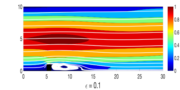
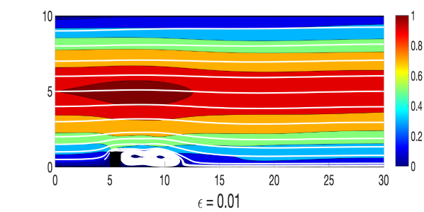
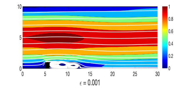
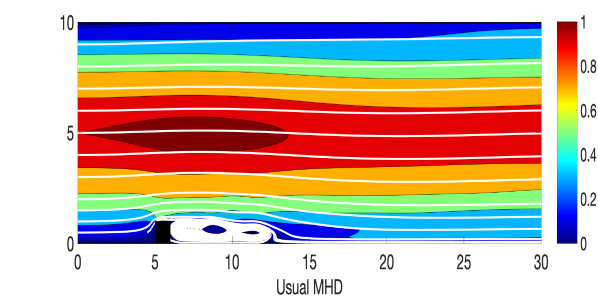
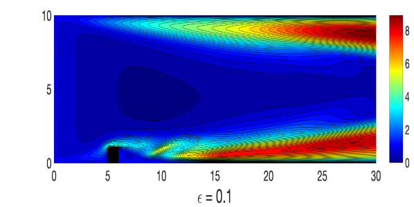
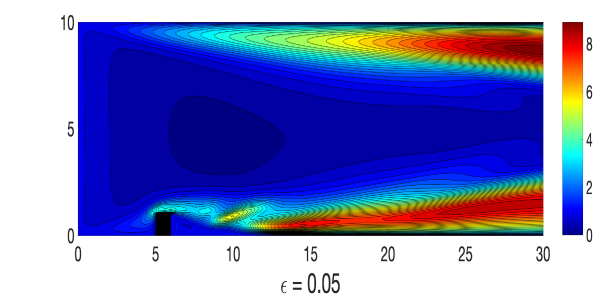
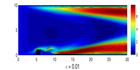
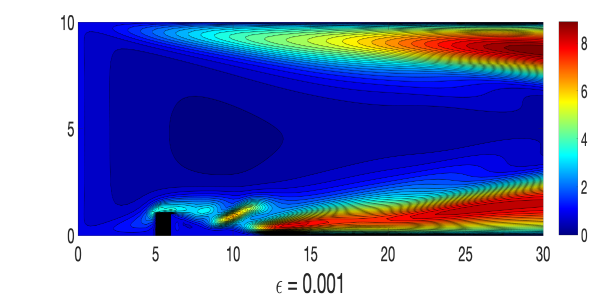
4.2 MHD channel flow over a step
Next, we consider a domain which is a rectangular channel with a step five units away from the inlet into the channel. No slip boundary condition is prescribed for the velocity and is enforced for the magnetic field on the walls. At the inflow, we set and , and the outflow condition uses a channel of extension 10 units, and at the end of the extension, we set outflow velocity and magnetic field equal to the inflow.
An ensemble of four different solutions corresponding to the perturbed initial conditions
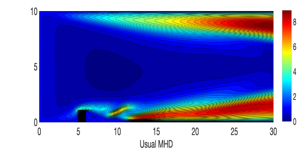
and where, , and , and a similar way perturbed inflow and outflow are considered. A triangular unstructured mesh of the domain that provides a total of 3316922 degrees of freedom (dof) is considered, where velocity , magnetic field , pressure , and magnetic pressure . The simulations of the Algorithm 3.1 are done with various values of until , with , , , , and timestep size . For the viscosity and magnetic diffusivity pair, we compute the largest possible so that the condition in (24) holds. Velocity and magnetic fields ensemble average solutions for varying and parameters are plotted in Figures 1-2, and compare them to the usual MHD simulation (which is the case). We observe that the ensemble average solutions appear to converge to the unperturbed solution as , which is expected from our theory.
Though, in our analysis, a timestep restriction appears due to the use of inverse inequality, in this numerical experiment, we could choose a larger timestep size and ran the simulation successfully for long time.

5 Conclusion and future works
In this paper, we proposed, analyzed, and tested a second order in time in practice, optimally accurate in space, decoupled and efficient algorithm for MHD flow ensemble computations. The second order temporal accuracy in practice is a major improvement to the first order ensemble average algorithm proposed in [47]. The algorithm extends the breakthrough idea for efficient computation of flow ensemble for Navier-Stokes [33] to MHD and combines with the breakthrough idea of Trenchea [59] to construct a decoupled stable scheme in terms of Elsässer variables. The key features to the efficiency of the algorithm are: (i) It is a stable decoupled method, split into two Oseen problems, which are identical to assembled, much easier to solve and can be solved simultaneously. (ii) At each time step, all different linear systems share the same coefficient matrix, as a result, the storage requirement is reduced, a single assembly of the coefficient matrix is required instead of times, preconditioners need to be built once and can be reused. (iii) It can take the advantage of the use of a block linear solver. (iv) No data restrictions are needed to avoid instability due to certain viscous terms. We proved the stability and second order convergence of the algorithm with respect to the timestep size. Numerical experiments were done on a unit square with a manufactured solution that verified the predicted convergence rates. Finally, we applied our scheme on a benchmark channel flow over a step problem and showed the method performed well. Though, in our analysis, a timestep restriction appears which was not observed in the numerical experiments.
In this paper, we considered the flow ensemble subject to the slightly different initial conditions and forcing functions, we plan to investigate flow ensemble behavior where the viscosities, and the boundary conditions involve uncertainties. In the numerical experiments, no timestep restriction was observed, and thus further investigation is needed to find unconditional stability of the scheme. The recent idea [20] of a continuous data assimilation algorithm for a velocity-vorticity formulation of the Navier-Stokes equations can be applied to the MHD flow ensemble. To reduce the computational cost, reduced order modeling (ROM) for the ensemble MHD flow computation will be the future research avenue. Recently, it has been shown the data-driven filtered ROM for flow problem [60] works well for the complex system. To reduced computation cost further to simulate an ensemble MHD system as well as more accurate results, it is worth exploring in ROM with physically accurate data [48]. We also plan to apply the recent advances [22] of an evolve-filter-relax based stabilization of ROMs for uncertainty quantification of the MHD flow ensemble using stochastic collocation method.
The finite element simulations of the Maxwell equations using nodal based elements often produce cancellation errors, interface problems [2], and spurious modes [11, 58] that cause unwanted and unphysical solutions. For magnetic field, the tangential components are continuous across inter-element boundaries but it is not necessary for the normal components. By the nature of finite-element interpolants, some nodal vectorial elements enforce the continuity of the normal component across the interface which is not required by the physics. It is now well established that the edge elements, are more appropriate for the finite element discretization of the Maxwell equations [3, 7, 10], which only enforces the tangential continuity of the magnetic field across the interfaces. MHD flow ensemble simulations with Nédélec’s edge element [51] will be the next research direction.
Acknowledgment. The author thanks Dr. Leo G. Rebholz for his constructive comments and suggestions that greatly improved the manuscript.
References
- [1] M. Akbas, S. Kaya, M. Mohebujjaman, and L. Rebholz. Numerical analysis and testing of a fully discrete, decoupled penalty-projection algorithm for MHD in elsässer variable. International Journal of Numerical Analysis Modeling, 13(1):90–113, 2016.
- [2] R. Albanese and G. Rubinacci. Analysis of three-dimensional electromagnetic fields using edge elements. Journal of Computational Physics, 108(2):236–245, 1993.
- [3] R. Albanese and G. Rubinacci. Finite element methods for the solution of 3D eddy current problems. Advances in Imaging and Electron Physics, 102:1–86, 1997.
- [4] D. Arnold and J. Qin. Quadratic velocity/linear pressure Stokes elements. In R. Vichnevetsky, D. Knight, and G. Richter, editors, Advances in Computer Methods for Partial Differential Equations VII, pages 28–34. IMACS, 1992.
- [5] L. Barleon, V. Casal, and L. Lenhart. MHD flow in liquid-metal-cooled blankets. Fusion Engineering and Design, 14:401–412, 1991.
- [6] J. D. Barrow, R. Maartens, and C.G. Tsagas. Cosmology with inhomogeneous magnetic fields. Physics Reports, 449:131–171, 2007.
- [7] R. Beck, R. Hiptmair, and B. Wohlmuth. Hierarchical error estimator for eddy current computation. Numerical mathematics and advanced applications (Jyväskylä, 1999), pages 110–120, 1999.
- [8] D. Biskamp. Magnetohydrodynamic Turbulence. Cambridge University Press, Cambridge, 2003.
- [9] P. Bodenheimer, G.P. Laughlin, M. Rozyczka, and H.W. Yorke. Numerical methods in astrophysics. Series in Astronomy and Astrophysics, Taylor Francis, New York, 2007.
- [10] A. Bossavit. A rationale for ‘edge-elements’ in 3-D fields computations. IEEE Transactions on Magnetics, 24(1):74–79, 1988.
- [11] A. Bossavit. Solving maxwell equations in a closed cavity, and the question of ‘spurious modes’. IEEE Transactions on magnetics, 26(2):702–705, 1990.
- [12] J. Brackbill and D. Barnes. The effect of nonzero on the numerical solution of the magnetohydrodynamics equations. Journal of Computational Physics, 35:426–430, 1980.
- [13] S. C. Brenner and L. R. Scott. The Mathematical Theory of Finite Element Methods, volume 15 of Texts in Applied Mathematics. Springer Science+Business Media, LLC, 2008.
- [14] M. Carney, P. Cunningham, J. Dowling, and C. Lee. Predicting probability distributions for surf height using an ensemble of mixture density networks. International Conference on Machine Learning, pages 113–120, 2005.
- [15] P. A. Davidson. An introduction to magnetohydrodynamics. Cambridge Texts in Applied Mathematics, Cambridge University Press, Cambridge, 2001.
- [16] E. Dormy and A. M. Soward. Mathematical aspects of natural dynamos. Fluid Mechanics of Astrophysics and Geophysics, Grenoble Sciences. Universite Joseph Fourier, Grenoble, VI, 2007.
- [17] P. P. Edwards, C.N.R Rao, N. Kumar, and A. S. Alexandrov. The possibility of a liquid superconductor. ChemPhysChem, 7(9):2015–2021, 2006.
- [18] J. A. Fiordilino. A second order ensemble timestepping algorithm for natural convection. SIAM Journal on Numerical Analysis, 56(2):816–837, 2018.
- [19] J. A. Font. Gerneral relativistic hydrodynamics and magnetohydrodynamics: hyperbolic system in relativistic astrophysics, in hyperbolic problems: theory, numerics, applications. Springer, Berlin, pages 3–17, 2008.
- [20] M. Gardner, A. Larios, L. G. Rebholz, D. Vargun, and C. Zerfas. Continuous data assimilation applied to a velocity-vorticity formulation of the 2D Navier-Stokes equations. American Institute of Mathematical Sciences Electronic Research Archive, to appear.
- [21] V. Girault and P.-A.Raviart. Finite element methods for Navier-Stokes equations: Theory and Algorithms. Springer-Verlag, 1986.
- [22] M. Gunzburger, T. Iliescu, M. Mohebujjaman, and M. Schneier. An evolve-filter-relax stabilized reduced order stochastic collocation method for the time-dependent Navier–Stokes equations. SIAM/ASA Journal on Uncertainty Quantification, 7(4):1162–1184, 2019.
- [23] M. Gunzburger, N. Jiang, and Z. Wang. A second-order time-stepping scheme for simulating ensembles of parameterized flow problems. Computational Methods in Applied Mathematics, 19:681–701, 2018.
- [24] H. Hashizume. Numerical and experimental research to solve MHD problem in liquid blanket system. Fusion Engineering and Design, 81:1431–1438, 2006.
- [25] F. Hecht. New development in Freefem++. Journal of Numerical Mathematics, 20:251–266, 2012.
- [26] T. Heister, M. Mohebujjaman, and L. Rebholz. Decoupled, unconditionally stable, higher order discretizations for MHD flow simulation. Journal of Scientific Computing, 71:21–43, 2017.
- [27] J. G. Heywood and R. Rannacher. Finite-element approximation of the nonstationary navier-stokes problem part iv: error analysis for second-order time discretization. SIAM Journal on Numerical Analysis, 27:353–384, 1990.
- [28] W. Hillebrandt and F. Kupka. Interdisciplinary aspects of turbulence. Lecture Notes in Physics, Springer-Verlag, Berlin, 756, 2009.
- [29] K. Hu, Y. Ma, and J. Xu. Stable finite element methods preserving exactly for MHD models. Numerische Mathematik, 135:371–397, 2017.
- [30] N. Jiang. A higher order ensemble simulation algorithm for fluid flows. Journal of Scientific Computing, 64:264–288, 2015.
- [31] N. Jiang. A second-order ensemble method based on a blended backward differentiation formula timestepping scheme for time-dependent Navier–Stokes equations. Numerical Methods for Partial Differential Equations, 33(1):34–61, 2017.
- [32] N. Jiang, S. Kaya, and W. Layton. Analysis of model variance for ensemble based turbulence modeling. Computational Methods in Applied Mathematics, 15:173–188, 2015.
- [33] N. Jiang and W. Layton. An algorithm for fast calculation of flow ensembles. International Journal for Uncertainty Quantification, 4:273–301, 2014.
- [34] N. Jiang and W. Layton. Numerical analysis of two ensemble eddy viscosity numerical regularizations of fluid motion. Numerical Methods for Partial Differential Equations, 31:630–651, 2015.
- [35] N. Jiang and M. Schneier. An efficient, partitioned ensemble algorithm for simulating ensembles of evolutionary MHD flows at low magnetic reynolds number. Numerical Methods for Partial Differential Equations, 34(6):2129–2152, 2018.
- [36] C. A. Jones and G. Schubert. Thermal and compositional convection in the outer core. Treatise in Geophysics, Core Dynamics, 8:131–185, 2015.
- [37] L. D. Landau and E. M. Lifshitz. Electrodynamics of Continuous Media. Pergamon Press, Oxford, 1960.
- [38] W. Layton. Introduction to the Numerical Analysis of Incompressible Viscous Flows. Computational Science and Engineering. Society for Industrial and Applied Mathematics, 2008.
- [39] J. M. Lewis. Roots of ensemble forecasting. Monthly Weather Review, 133:1865 – 1885, 2005.
- [40] Y. Li and C. Trenchea. Partitioned second order method for magnetohydrodynamics in elsässer variables. Discrete & Continuous Dynamical Systems-B, 23(7):2803, 2018.
- [41] T. F. Lin, J. B. Gilbert, and R. Kossowsky. Sea-water magnetohydrodynamic propulsion for next-generation undersea vehicles. Technical report, PENNSYLVANIA STATE UNIV STATE COLLEGE APPLIED RESEARCH LAB, 1990.
- [42] T. N. Palmer M. Leutbecher. Ensemble forecasting. Journal of Computational Physics, 227:3515–3539, 2008.
- [43] O. P. L. Maître and O. M. Knio. Spectral methods for uncertainty quantification. Springer, 2010.
- [44] W. J. Martin and M. Xue. Sensitivity analysis of convection of the 24 May 2002 IHOP case using very large ensembles. Monthly Weather Review, 134(1):192–207, 2006.
- [45] D. L. Mitchell and D. U. Gubser. Magnetohydrodynamic ship propulsion with superconducting magnets. Journal of Superconductivity, 1(4):349–364, 1988.
- [46] M. Mohebujjaman. Efficient numerical methods for magnetohydrodynamic flow. Ph.D. Thesis, Clemson University, 2017.
- [47] M. Mohebujjaman and L. G. Rebholz. An efficient algorithm for computation of MHD flow ensembles. Computational Methods in Applied Mathematics, 17:121–137, 2017.
- [48] M. Mohebujjaman, L. G. Rebholz, and T. Iliescu. Physically-constrained data-driven, filtered reduced order modeling of fluid flows. International Journal for Numerical Methods in Fluids, accepted.
- [49] M. Mohebujjaman, S. Shiraiwa, B. LaBombard, J. C. Wright, and K. Uppalapati. Scalability analysis of direct and iterative solvers used to model charging of non-insulated superconducting pancake solenoids. arXiv preprint arXiv:2007.15410, 2020.
- [50] M. Neda, A. Takhirov, and J. Waters. Ensemble calculations for time relaxation fluid flow models. Numerical Methods for Partial Differential Equations, 32(3):757–777, 2016.
- [51] J. C. Nédélec. Mixed finite elements in . Numerische Mathematik, 35(3):315–341, 1980.
- [52] P. Olson. Experimental dynamos and the dynamics of planetary cores. Annual Review of Earth and Planetary Sciences, 41:153–181, 2013.
- [53] J. D. G. Osorio and S. G. G. Galiano. Building hazard maps of extreme daily rainy events from PDF ensemble, via REA method, on Senegal river basin. Hydrology and Earth System Sciences, 15:3605 – 3615, 2011.
- [54] B. Punsly. Black hole gravitohydrodynamics. Astrophysics and Space Science Library, Springer-Verlag, Berlin, Second Edition, 355, 2008.
- [55] M. A. Samad and M. Mohebujjaman. MHD heat and mass transfer free convection flow along a verticle stretching sheet in presence of magnetic field with heat generation. Research Journal of Applied Sciences, Engineering and Technology, 1(3):98–106, 2009.
- [56] L. R. Scott and M. Vogelius. Conforming finite element methods for incompressible and nearly incompressible continua. Lectures in Applied Mathematics, 22(2), 1985.
- [57] S. Smolentsev, R. Moreau, L. Buhler, and C. Mistrangelo. MHD thermofluid issues of liquid-metal blankets: phenomena and advances. Fusion Engineering and Design, 85:1196–1205, 2010.
- [58] D. Sun, J. Manges, X. Yuan, and Z. Cendes. Spurious modes in finite-element methods. IEEE Antennas and Propagation Magazine, 37(5):12–24, 1995.
- [59] C. Trenchea. Unconditional stability of a partitioned IMEX method for magnetohydrodynamic flows. Applied Mathematics Letters, 27:97–100, 2014.
- [60] X. Xie, M. Mohebujjaman, L. G. Rebholz, and T. Iliescu. Data-driven filtered reduced order modeling of fluid flows. SIAM Journal on Scientific Computing, 40(3):B834–B857, 2018.
- [61] S. Zhang. A new family of stable mixed finite elements for the 3D Stokes equations. Mathematics of Computation, 74:543–554, 2005.