High-order finite element method for atomic structure calculations
Computational Physics and Methods (CCS-2)
Los Alamos National Laboratory
NM 87545, USA
ondrej@certik.us &John E. Pask
Physics Division
Lawrence Livermore National Laboratory
Livermore, CA 94550, USA
pask1@llnl.gov &
Department of Computer Science
University of Illinois at Urbana–Champaign
Urbana, IL 61801, USA isuruf@gmail.com &
Science Institute, University of Iceland
Quansight Labs, TX, Austin
rgoswami@ieee.org &N. Sukumar
Department of Civil and Environmental Engineering
University of California, Davis
CA 95616, USA
nsukumar@ucdavis.edu &
Physics and Chemistry of Materials (T-1)
Los Alamos National Laboratory
NM 87545, USA
lac@lanl.gov &Gianmarco Manzini
Applied Mathematics and Plasma Physics (T-5)
Los Alamos National Laboratory
NM 87545, USA
gmanzini@lanl.gov &
Institute of Physics
Academy of Sciences of the Czech Republic
Na Slovance 2, 182 21 Praha 8, Czech Republic
vackar@fzu.cz
Abstract
We introduce featom, an open source code that implements a high-order finite element solver for the radial Schrödinger, Dirac, and Kohn-Sham equations. The formulation accommodates various mesh types, such as uniform or exponential, and the convergence can be systematically controlled by increasing the number and/or polynomial order of the finite element basis functions. The Dirac equation is solved using a squared Hamiltonian approach to eliminate spurious states. To address the slow convergence of the states due to divergent derivatives at the origin, we incorporate known asymptotic forms into the solutions. We achieve a high level of accuracy ( Hartree) for total energies and eigenvalues of heavy atoms such as uranium in both Schrödinger and Dirac Kohn-Sham solutions. We provide detailed convergence studies and computational parameters required to attain commonly required accuracies. Finally, we compare our results with known analytic results as well as the results of other methods. In particular, we calculate benchmark results for atomic numbers () from 1 to 92, verifying current benchmarks. We demonstrate significant speedup compared to the state-of-the-art shooting solver dftatom. An efficient, modular Fortran 2008 implementation, is provided under an open source, permissive license, including examples and tests, wherein particular emphasis is placed on the independence (no global variables), reusability, and generality of the individual routines.
Keywords atomic structure, electronic structure, Schrödinger equation, Dirac equation, Kohn-Sham equations, density functional theory, finite element method, Fortran 2008
1 Introduction
Over the past three decades, Density Functional Theory (DFT) [1] has established itself as a cornerstone of modern materials research, enabling the understanding, prediction, and control of a wide variety of materials properties from the first principles of quantum mechanics, with no empirical parameters. However, the solution of the required Kohn-Sham equations [2] is a formidable task, which has given rise to a number of different solution methods [3]. At the heart of the majority of methods in use today, whether for isolated systems such as molecules or extended systems such as solids and liquids, lies the solution of the Schrödinger and/or Dirac equations for the isolated atoms composing the larger molecular or condensed matter systems of interest. Particular challenges arise in the context of relativistic calculations, which require solving the Dirac equation, since spurious states can arise due to the unbounded nature of the Dirac Hamiltonian operator and inconsistencies in discretizations derived therefrom [4].
A number of approaches have been developed to avoid spurious states in the solution of the Dirac equation. Shooting methods, e.g., [5] and references therein, avoid such states by leveraging known asymptotic forms to target desired eigenfunctions based on selected energies and numbers of nodes. However, due to the need for many trial solutions to find each eigenfunction, efficient implementation while maintaining robustness is nontrivial. In addition, convergence parameters such as distance of grid points from the origin must be carefully tuned. Basis set methods, e.g., [6, 7, 8, 9] and references therein, offer an elegant alternative to shooting methods, solving for all states at once by diagonalization of the Schrödinger or Dirac Hamiltonian in the chosen basis. However, due to the unbounded spectrum of the Dirac Hamiltonian, spurious states have been a longstanding issue [4, 10]. Many approaches have been developed to avoid spurious states over the past few decades, with varying degrees of success. These include using different bases for the large and small components of the Dirac wavefunction [6, 11, 12, 7, 13, 14], modifying the Hamiltonian [15, 8, 9, 16, 17], and imposing various boundary constraints [18, 19, 12, 8]. In the finite-difference context, defining large and small components of the Dirac wavefunction on alternate grid points [20], replacing conventional central differences with asymmetric differences [20, 21], and adding a Wilson term to the Hamiltonian [17] have proven effective in eliminating spurious states. While in the finite element (FE) context, the use of different trial and test spaces in a stabilized Petrov-Galerkin formulation has proven effective in mitigating the large off-diagonal convection (first derivative) terms and absence of diffusion (second derivative) terms causing the instability [9, 16].
In the this work, we present the open-source code,featom111Source also publicly on Github: https://github.com/atomic-solvers/featom, for the solution of the Schrödinger, Dirac, and Kohn-Sham equations in a high-order finite element basis. The FE basis enables exponential convergence with respect to polynomial order while allowing full flexibility as to choice of radial mesh. To eliminate spurious states in the solution of the Dirac equation, we square the Dirac Hamiltonian operator [22, 15]. Since the square of the operator has the same eigenfunctions as the operator itself, and the square of its eigenvalues, determination of the desired eigenfunctions and eigenvalues is immediate. Most importantly, since the square of the operator is bounded from below, unlike the operator itself, it is amenable to direct solution by standard variational methods, such as FE, without modification. This affords simplicity, robustness, and well understood convergence. Moreover, squaring the operator rather than modifying it and/or boundary conditions upon it, ensures key properties are preserved exactly, such as convergence to the correct non-relativistic (Schrödinger) limit with increasing speed of light [15]. Squaring the operator also stabilizes the numerics naturally, without approximation, by creating second-derivative terms. To accelerate convergence with respect to polynomial order, we incorporate known asymptotic forms as into the solutions: rather than solving for large and small Dirac wavefunction components and , we solve for and , with based on the known asymptotic forms for and as . This eliminates derivative divergences and non-polynomial behavior in the vicinity of the origin and so enables rapidly convergent solutions in a polynomial basis for all quantum numbers , including . By combining the above ideas, featom is able to provide robust, efficient, and accurate solutions for both Schrödinger and Dirac equations.
The package is MIT licensed and is written in Fortran, leveraging language features from the 2008 standard, with an emphasis on facilitating user extensions. Additionally, it is designed to work within the modern Fortran ecosystem and leverages the fpm build system. There are several benchmark calculations that serve as tests. The package supports different mesh-generating methods, including support for a uniform mesh, an exponential mesh, and other meshes defined by nodal distributions and derivatives. Multiple quadrature methods have been implemented, and their usage in the code is physically motivated. Gauss–Jacobi quadrature is used to accurately integrate problematic integrals for the Dirac equation and the Poisson equation as well as for the total energy in the Dirac-Kohn-Sham solution, whereas Gauss–Legendre quadrature is used for the Schrödinger equation. To ensure numerical accuracy, we employ several techniques, using Gauss–Lobatto quadrature for the overlap matrix to recover a standard eigenproblem, precalculation of most quantities, and parsimonious assembly of a lower-triangular matrix with a symmetric eigensolver. With these considerations we show that the resulting code outperforms the state-of-the-art code dftatom, using fewer parameters for convergence while retaining high accuracy of Hartree in total energy and eigenvalues for uranium (both Dirac and Schrödinger) and all lighter atoms.
The remainder of the paper is organized as follows. Section 2 describes the electronic structure equations solved. This is followed by Sections 3.1 and 3.2, which detail the unified finite element solution for the radial Schrödinger and Dirac equations. Section 4.4 details the numerical techniques employed to efficiently construct and solve the resulting matrix eigenvalue problem, including mesh and quadrature methods. In Section 4, we present results from analytic tests and benchmark comparisons against the shooting solver dftatom, followed by a brief discussion of findings. Finally, in Section 5, we summarize our main conclusions.
2 Electronic structure equations
Under the assumption of a central potential, we establish the conventions used for the electronic structure problems under the purview of featom in this section. Starting from the nonrelativistic radial Schrödinger equation and its relativistic counterpart, the Dirac equation, we couple these to the Kohn–Sham equations with a Poisson equation for the Hartree potential. The interested reader may find more details of this formulation in [5]. By convention, we use Hartree atomic units throughout the manuscript.
2.1 Radial Schrödinger equation
Recall that the 3D one-electron Schrödinger equation is given by
| (1) |
When the potential considered is spherically symmetric, i.e.,
| (2) |
the eigenstates of energy and angular momentum can be written in the form
| (3) |
where is the principal quantum number, is the orbital angular momentum quantum number, and is the magnetic quantum number. It follows that satisfies the radial Schrödinger equation
| (4) |
The functions and are normalized as
| (5) |
2.2 Radial Dirac equation
The one-electron radial Dirac equation can be written as
| (6a) | ||||
| (6b) | ||||
where and are related to the usual large and small components of the Dirac equation by
| (7a) | ||||
| (7b) | ||||
A pedagogical derivation of these results can be found in the literature, for example in [5, 23, 24]. We follow the solution labeling in [5], in which the relativistic quantum number is determined by the orbital angular momentum quantum number and spin quantum number on the basis of the total angular momentum quantum number using
| (8) |
By not including the rest mass energy of an electron, the energies obtained from the radial Dirac equation can be compared to the non-relativistic energies obtained from the Schrödinger equation.
The normalization of and is
| (9) |
We note that both and are solutions of homogeneous equations and are thus only unique up to an arbitrary multiplicative constant.
2.3 Poisson equation
The 3D Poisson equation for the Hartree potential due to electronic density is given by
| (10) |
For a spherical density , this becomes
| (11) |
where is the radial particle (number) density, normalized such that
| (12) |
where is the number of electrons.
2.3.1 Initial conditions
Substituting (11) into (12) and integrating, we obtain
| (13) |
from which it follows that the asymptotic behavior of is
| (14) |
Integrating (14) and requiring as then gives the corresponding asymptotic behavior for ,
| (15) |
For small , the asymptotic behavior can be obtained by expanding about : . Substituting into Poisson equation (11) gives
| (16) |
Integrating and requiring to be finite then gives
| (17) |
with linear leading term, so that we have
| (18) |
Integrating (17) then gives
| (19) |
with leading constant term determined by Coulomb’s law:
| (20) |
Finally, from (18) we have that
| (21) |
So as and . This asymptotic behavior provides the initial values and derivatives for numerical integration in both inward and outward directions.
2.4 Kohn-Sham equations
The Kohn–Sham equations consist of the radial Schrödinger or Dirac equations with an effective potential given by (see, e.g., [3])
| (22) |
where is the Hartree potential given by the solution of the radial Poisson equation (11), is the exchange-correlation potential, and is the nuclear potential.
The total energy is given by
| (23) |
the sum of kinetic energy
| (24) |
where are the Kohn-Sham eigenvalues, Hartree energy
| (25) |
exchange-correlation energy
| (26) |
where is the exchange and correlation energy density, and Coulomb energy
| (27) |
with electronic density in the nonrelativistic case given by
| (28) |
where is the radial wavefunction in (40) and the associated electronic occupation. In the relativistic case, the electronic density is given by
| (29) |
where and are the two components of the Dirac solution ((6a), (6b)) and is the occupation. In both the above cases, is the electronic particle density [electrons/volume], everywhere positive, as distinct from the electronic charge density [charge/volume]: in atomic units.
We adopt a self-consistent approach [3] to solve for the electronic structure. Starting from an initial density and corresponding potential , we solve the Schrödinger or Dirac equation to determine the wavefunctions or spinor components and , respectively. From these, we construct a new density and potential . Subsequently, we update the input density and potential, using for example a weighting parameter :
| (30) | |||
| (31) |
This process is repeated until the difference of and and/or and is within a specified tolerance, at which point self-consistency is achieved. This fixed-point iteration is known as the self-consistent field (SCF) iteration. We employ an adaptive linear mixing scheme, with optimized weights for each component of the potential to construct new input potentials for successive SCF iterations. To accelerate the convergence of the SCF iterations, under relaxed fixed point iteration methods are used. In particular, the code supports both linear [25] and (default) Periodic Pulay mixing schemes [26], which suitably accelerate convergence. In order to reduce the number of SCF iterations, we use a Thomas–Fermi (TF) approximation [27] for the initial density and potential:
| (32a) | |||
| (32b) | |||
| (32c) | |||
| (32d) | |||
The corresponding charge density is then
| (33) |
We demonstrate the methodology with the local density approximation (LDA) and relativistic local-density approximation (RLDA) exchange and correlation functionals. We note that the modular nature of the code and interface mechanism make it straightforward to incorporate functionals from other packages such as the library of exchange correlation functions, libxc [28, 29]. The parameters used in featom are taken from the same NIST benchmark data [30] as the current state-of-the-art dftatom program for an accurate comparison. For the local density approximation,
| (34) |
where the exchange and correlation energy density can be written as [3]
| (35) |
with electron gas exchange term [3]
| (36) |
and Vosko-Wilk-Nusair (VWN) [31] correlation term
| (37) |
in which , , , , , , , and
| (38) |
is the Wigner-Seitz radius, which gives the mean distance between electrons. In the relativistic (RLDA) case, a correction to the LDA exchange energy density and potential is given by MacDonald and Vosko [32]:
| (39a) | |||
| (39b) | |||
where and .
3 Solution methodology
Having described the Schrödinger, Dirac, and Kohn-Sham electronic structure equations to be solved, and key solution properties, we now detail our approach to solutions in a high-order finite-element basis.
3.1 Radial Schrödinger equation
To recast (4) in a manner that will facilitate our finite element solution methodology, we make the substitution to obtain the canonical radial Schrödinger equation in terms of is
| (40) |
The corresponding normalization of is
| (41) |
3.1.1 Asymptotics
The known asymptotic behavior of as is [33]
| (42) |
where , being a solution of a homogeneous system of equations, is only unique up to an arbitrary multiplicative constant. We use (40) as our starting point but from now on drop the index from for simplicity:
| (43) |
In order to facilitate rapid convergence and application of desired boundary conditions in a finite element basis, we generalize (40) to solve for for any chosen real exponent by substituting to obtain
| (44) |
We note that:
3.1.2 Weak form
To obtain the weak form, we multiply both sides of (44) by a test function and integrate from to . In addition, to facilitate the construction of a symmetric bilinear form, we multipy by a factor to get
| (46) | |||
We can now integrate by parts to obtain
| (47) | |||
Setting the boundary term to zero,
| (48) |
we then obtain the desired symmetric weak formulation
| (49) | |||
As discussed below, by virtue of our choice of and boundary conditions on , the vanishing of the boundary term (48) imposes no natural boundary conditions on .
3.1.3 Discretization
To discretize (49), we introduce finite element basis functions to form trial and test functions
| (50) |
and substitute into (49). In so doing, we obtain a generalized eigenvalue problem
| (51) |
where is the Hamiltonian matrix,
| (52) |
and is the overlap matrix,
| (53) |
3.1.4 Basis
While, by virtue of the weak formulation, the above discretization can employ any basis in Sobolev space satisfying the required boundary conditions (including standard FE bases, Hermite, and B-splines), we employ a high-order spectral element (SE) basis [34,35] in the present work. FE bases consist of local piecewise polynomials. SE bases are a form of FE basis constructed to enable well-conditioned, high polynomial-order discretization via definition over Lobatto nodes rather than uniformly spaced nodes within each finite element (mesh interval). In the present work, we employ polynomial orders up to .
In the electronic structure context, SE bases have a number of desirable properties, including:
-
1.
Polynomial completeness and associated systematic convergence with increasing number and/or polynomial order of basis functions.
-
2.
Well conditioned to high polynomial order by virtue of definition over Lobatto nodes.
-
3.
Exponential convergence with respect to polynomial order, enabling high accuracy with a small basis.
-
4.
Applicable to general nonsingular as well as singular Coulombic potentials, whether fixed or self-consistent.
-
5.
Applicable to bound as well as excited states.
-
6.
Can use uniform as well as nonuniform meshes.
-
7.
Basis function evaluation, differentiation, and integration are inexpensive, enabling fast and accurate matrix element computations.
-
8.
Dirichlet boundary conditions are readily imposed by virtue of cardinality, i.e.,
where is a nodal point of the basis.
-
9.
Derivative boundary conditions are readily imposed via the weak formulation.
-
10.
Diagonal overlap matrix using Lobatto quadrature, thus enabling solution of a standard rather than generalized eigenvalue problem, reducing both storage requirements and time to solution.
Properties (1)-(4), (7), and (10) are advantageous relative to Slater-type and Gaussian-type bases, which can be nontrivial to converge; can become ill-conditioned as the number of basis functions is increased, limiting accuracies attainable in practice; and produce a non-diagonal overlap matrix, requiring solution of a generalized rather than standard matrix eigenvalue problem.
Properties (2) and (10) are advantageous relative to B-spline bases, which are generally employed at lower polynomial orders in practice and give rise to a non-diagonal overlap matrix, thus requiring solution of a generalized rather than standard matrix eigenvalue problem.
3.1.5 Boundary conditions
Since we seek bound states, which vanish as , we impose a homogeneous Dirichlet boundary condition on and at by employing a finite element basis satisfying this condition.
For , at for all quantum numbers according to (42). Thus we impose a homogeneous Dirichlet boundary condition on and at by employing a finite element basis satisfying this condition, whereupon the boundary term (48) as a whole vanishes, consistent with the weak formulation (49).
For , at for all quantum numbers according to (42). However, at for . Thus a homogeneous Dirichlet boundary condition cannot be imposed for . However, for , the factor in (48) vanishes at , whereupon the boundary term as a whole vanishes, consistent with the weak formulation (49), regardless of boundary condition on and at . Hence for , we impose a homogeneous Dirichlet boundary condition on and at only, by employing a finite element basis satisfying this condition. This is sufficient due to the singularity of the associated Sturm-Liouville problem.
Similarly, for , at for all quantum numbers according to (42) and, since , we again impose a homogeneous Dirichlet boundary condition on and at only.
In practice, the featom code defaults to with homogeneous Dirichlet boundary conditions at and .
Note that, while yields a rapidly convergent formulation in the context of the Schrödinger equation, it does not suffice in the context of the Dirac equation, as discussed in Section 3.2.4.
3.2 Radial Dirac equation
For small , the central potential has the form , which gives rise to the following asymptotic behavior at the origin for (Coulombic) [34, 24]:
| (54a) | |||
| (54b) | |||
| (54c) | |||
For (nonsingular) the asymptotic is, for [34]
| (55a) | ||||
| (55b) | ||||
and for
| (56a) | ||||
| (56b) | ||||
For large , assuming as , the asymptotic is [33]
| (57a) | |||
| (57b) | |||
| (57c) | |||
Consistent with the coupled equations (6a) and (6b), the Dirac Hamiltonian can be written as (see, e.g., [7, (7)])
| (58) |
The corresponding eigenvalue problem is then
| (59) |
To discretize, we expand the solution vector in a basis:
| (60) |
where and denote the upper and lower components of the vector. We have basis functions (degrees of freedom), for each wave function component. As such, the function is expanded in terms of basis functions and the function in terms of . However, these two expansions are not independent but are rather coupled via coefficients .
3.2.1 Squared Hamiltonian formulation
The above eigenvalue formulation of the radial Dirac equation can be solved using the finite element method. However, due to the fact that the operator is not bounded from below, one obtains spurious eigenvalues in the spectrum [10]. To eliminate spurious states, we work with the square of the Hamiltonian [22, 15], which is bounded from below, rather than the Hamiltonian itself. Since the eigenfunctions of the square of an operator are the same as those of the operator itself, and the eigenvalues are the squares, the approach is straightforward and enables direct and efficient solution by the finite element method.
Let us derive the equations for the squared radial Dirac Hamiltonian. First we shift the energy by to obtain the relativistic energy, making the Hamiltonian more symmetric, using (58) to get
| (61) |
Then we square the Hamiltonian using (59) to obtain the following equations to solve for and :
| (62) |
where is the identity matrix.
As can be seen, the eigenvectors and are the same as before but the eigenvalues are now equal to and the original non-relativistic energies can be obtained by taking the square root of these new eigenvalues and subtracting .
3.2.2 Weak form
We follow a similar approach as for the Schrödinger equation: instead of solving for and , we solve for and , which introduces a parameter that can be chosen to facilitate rapid convergence and the application of the desired boundary conditions in a finite element basis. We then multiply the eigenvectors by to obtain and .
Now we can write the finite element formulation as
| (63a) | ||||
| (63b) | ||||
| (63c) | ||||
This is a generalized eigenvalue problem, with eigenvectors (coefficients of ), eigenvalues , and block matrices and . Note that the basis functions from both sides were multiplied by due to the substitutions and . We can denote the middle factor in the integral for as and compute it using (61) with rearrangement of factors as follows:
| (64a) | ||||
| (64b) | ||||
Let
| (65) |
Then
| (66a) | ||||
| (66b) | ||||
| (66c) | ||||
| (66d) | ||||
where .
The full derivation of these expressions is given in A.1.
The usual approach when applying the finite element method to a system of equations is to choose the basis functions in the following form:
| (67a) | ||||
| (67b) | ||||
Substituting (67) into (63), we obtain the following expressions after simplification (A.2):
| (68a) | ||||
| (68b) | ||||
with components given by
| (69a) | ||||
| (69b) | ||||
| (69c) | ||||
| (69d) | ||||
| (69e) | ||||
where .
These are the expressions implemented in the featom code.
3.2.3 Basis
Because we solve the squared Dirac Hamiltonian problem (62), whose spectrum has a lower bound, rather than the Dirac Hamiltonian problem (59), whose spectrum is unbounded above and below, we can employ a high-order SE basis [35, 36], as in the Schrödinger case, as discussed in Section 3.1.5, with exponential convergence to high accuracy and no spurious states.
As discussed in Section 1, a number of approaches have been developed over the past few decades to solve (59) directly without spurious states, with varying degrees of success. Perhaps most common is to use different bases for large and small components, and , of the Dirac wavefunction, e.g., [6, 11, 12, 7, 13, 14]. And among these approaches, perhaps most common is to impose some form of “kinetic balance,” e.g., [13, 4] and references therein, on the bases for and . However, imposing such conditions significantly complicates the basis, increasing the cost of evaluations and matrix element integrals, and while highly effective in practice is not guaranteed to eliminate spurious states all cases [13]. In any case, for a basis as employed in the present work, such balance cannot be imposed since it produces basis functions which are discontinuous and thus not in Sobolev space as required (Section 3.1.5). Another approach which has proven successful in the context of B-spline bases is to use different orders of B-splines as bases for and [7, 37, 38].
However, this too creates additional complexity [38], did not eliminate all spurious states in our implementation using and degree SE bases for and , respectively, nor eliminate all spurious states in previous work [39]. Thus we opt instead for the squared Hamiltonian approach in the present work in order to allow the robust and efficient use of a high-order SE basis, with all desired properties enumerated in Section 3.1.5. In addition, the squared Hamiltonian approach allows direct solution for just the positive (electron) states, rather than having to solve for both positive and negative, e.g., [37], thus saving computation.
Finally, as discussed in Section 3.2.4, we note that by solving for and , with set according to the known asymptotic as , rather than for and themselves, we obtain rapid convergence for singular Coulomb as well as nonsingular potentials using our SE basis. On the other hand, singular Coulomb potentials have posed significant difficulty for B-spline bases [37]. However, since B-splines have polynomial completeness to specified degree, like SE bases, solving for and rather than and directly should yield rapid convergence for such singular potentials using B-spline bases as well.
3.2.4 Boundary conditions
To construct a symmetric weak form, the following two boundary terms are set to zero in the derivation (A.2):
| (70a) | ||||
| (70b) | ||||
As in the Schrödinger case, since we seek bound states which vanish as , we impose a homogeneous Dirichlet boundary condition on the test function and solutions and at by employing a finite element basis satisfying this condition.
Unlike the Schrödinger case, however, the appropriate exponent and boundary condition at depends on the regularity of the potential .
For nonsingular potentials , and as for relativistic quantum numbers while and for according to (55) and (56). Hence, as in the Schrödinger case, for , and at for all quantum numbers and . Thus we impose a homogeneous Dirichlet bounday condition on , , and at by employing a finite element basis satisfying this condition, whereupon the boundary terms (70) vanish, consistent with the weak formulation (63). This is the default in the featom code for such potentials.
For singular potentials with leading term (Coulombic), however, and have leading terms varying as as for all relativistic quantum numbers according to (54). However, while for , we have for (for ), so that and have non-polynomial behavior at small and divergent derivatives at , leading to numerical difficulties for methods attempting to compute them directly. To address this issue, we leverage the generality of the formulation (63) to solve for and with , rather than solving for and directly. With , and have polynomial behavior at small and bounded nonzero values at for all , including , thus eliminating the aforementioned numerical difficulties completely and facilitating rapid convergence in a polynomial basis. Finally, for , the factors in the boundary terms (70) vanish at , whereupon the boundary terms as a whole vanish, consistent with the weak formulation (63), regardless of boundary condition on , , and at . Hence, for , we impose a homogeneous Dirichlet boundary condition at only, by employing a finite element basis satisfying this condition. This is the default in the featom code for such potentials.
For integrals involving non-integer , we employ Gauss-Jacobi quadrature for accuracy and efficiency, while for integrals involving only integer exponents, we use Gauss-Legendre quadrature with the exception of overlap integrals where we employ Gauss-Lobatto quadrature to obtain a diagonal overlap matrix.
4 Results and discussion
To demonstrate the accuracy and performance of the featom implementation of the above described finite element formulation, we present results for fixed potentials as well as self-consistent DFT calculations, with comparisons to analytic results where available and to the state-of-the-art dftatom solver otherwise. Code outputs are collected in B.
4.1 Coulombic systems
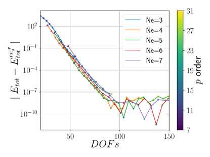
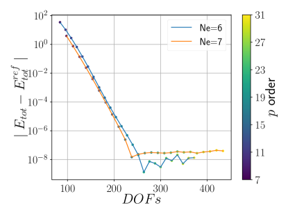
The accuracy of the Schrödinger and Dirac solvers was verified using the Coulomb potential for (uranium). Eigenvalues are given by the corresponding analytic formula [5]. All eigenvalues with are used for the study. The reference eigenvalues here are from the analytic solutions: for the Schrödinger equation, and
| (71a) | ||||
| (71b) | ||||
for the Dirac equation.
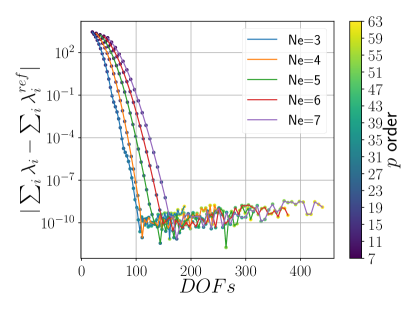
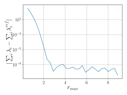
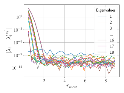
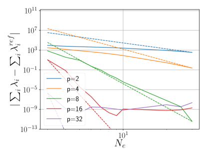
Figure 1a shows the convergence of the Schrödinger total energy error with respect to the polynomial order for different numbers of elements . The graph, when observed for a given number of elements, forms a straight line on the log-linear scale, showing that the error decreases exponentially with the polynomial order until it reaches the numerical precision limit of approximately .
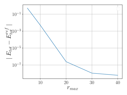
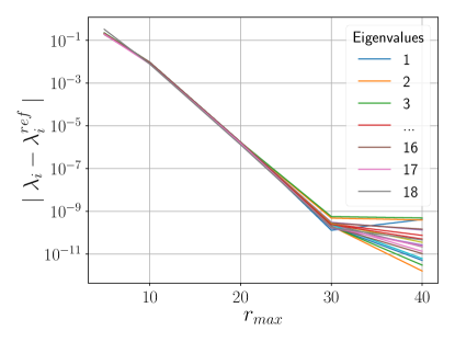
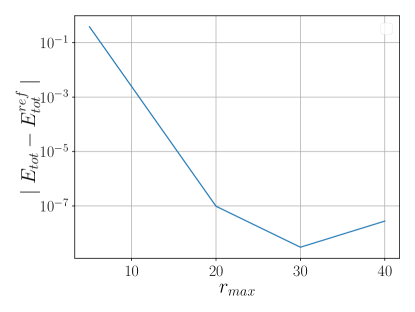
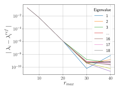
For five elements, we considered the behavior of the error with respect to . Figure 1b shows the total energy error. It is observed that results in an error of or less. The eigenvalues converge to for , as depicted in Figure 1c.
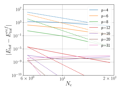
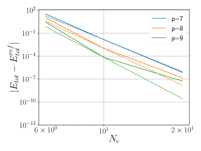
The theoretical convergence rate for the finite element method is given by . Figure 1d shows the error with respect to , juxtaposed with the theoretical convergence represented as a dotted line. The slope of the solid lines is used to determine the rate of convergence. In all instances, we observe that the theoretical convergence rate is achieved. For polynomial orders , it is attained asymptotically, while for , it approaches the limiting numerical precision of around .
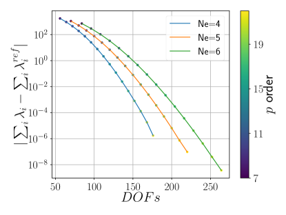
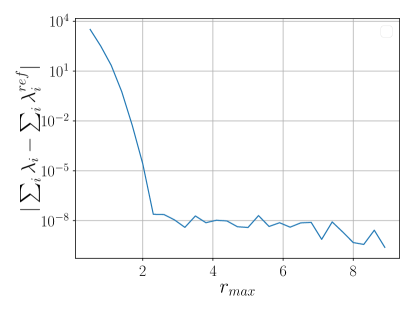
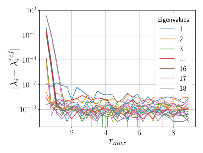
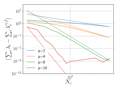
Figure 2a shows the error in the Dirac total energy with respect to for various . We find the same exponential relationship between the error and polynomial order .
As before, for five elements, we consider the error with respect to . Figure 2b shows the total Dirac energy error, and it is observed that results in an error of or less. The eigenvalues converge to for , as depicted in Figure 2c.
Figure 2d shows the error as is increased alongside the theoretical convergence represented as a dotted line. In all instances, we observe that the theoretical convergence rate is achieved. For polynomial orders , it is attained asymptotically, while for , it approaches the limiting numerical precision of around .
4.2 Quantum harmonic oscillator
Next, we consider a nonsingular potential: the harmonic oscillator potential given by . For the Schrödinger equation, we take and compare against the exact values given by
| (72) |
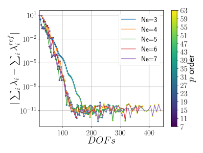
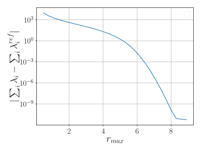
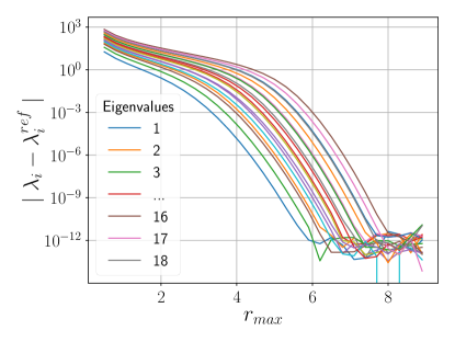
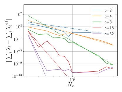
Figure 3a shows the total Schrödinger energy error with respect to the polynomial order for various values. For fixed , the straight line on the log-linear graph shows the exponential dependency of the error on until hitting the numerical precision limit ( ).
The effect of on the error was tested with five elements. Figure 3b indicates that gives a total energy error of or lower. Figure 3c shows that the eigenvalues converge to under the same condition.
The dependence of the error on , together with the theoretical convergence rate (), is shown in Figure 3d. The slope of the solid lines confirms that the theoretical convergence rate is achieved. It is asymptotically achieved for , while for , it approaches the limiting numerical precision of approximately .
For the Dirac equation, comparisons are with respect to dftatom results.
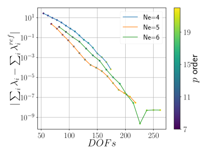
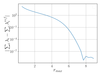
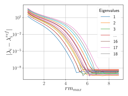
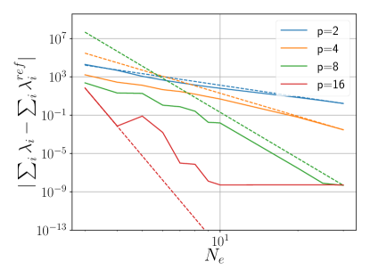
Figure 4a shows an exponential error decrease with respect to for various . A similar pattern is observed with , reducing the total Dirac energy error to or less (Figure 4b). Eigenvalue convergence to is also seen (Figure 4c).
The theoretical convergence rate () is confirmed in Figure 4d, attained asymptotically for and reaching a numerical precision limit of for .
4.3 DFT calculations
The accuracy of the DFT solvers using both Schrödinger and Dirac equations is compared against dftatom results for the challenging case of uranium. The non-relativistic Schrödinger calculation yields the following electronic configuration:
With the Dirac solver, the -shell occupation splits according to the degeneracy of the and subshells.
Figures 5a and 6a demonstrate an exponential decrease in total energy error with increasing for various . As increases to for five elements, the error decreases to or less (Figures 5b and 6b). Convergence of eigenvalues to is seen at (Figures 5c and 6c).
In Figures 5d and 6d, the theoretical convergence rate () manifests when , below which numerical instabilities prevent convergence.
4.4 Numerical considerations
The mesh parameters used to achieve a.u. accuracy for the DFT Schrödinger and Dirac calulations are shown in Table 1. The mesh parameters used for a.u. accuracy are shown in Table 2.
| Parameter | DFT Schrödinger | Dirac |
|---|---|---|
| 92 | 92 | |
| 0 | 0 | |
| 50 | 30 | |
| 200 | 600 | |
| 4 | 6 | |
| 53 | 64 | |
| 26 | 25 | |
| — | 0.005 |
| Parameter | DFT Schrödinger | Dirac |
|---|---|---|
| 92 | 92 | |
| 0 | 0 | |
| 30 | 30 | |
| 200 | 100 | |
| 4 | 5 | |
| 35 | 40 | |
| 17 | 24 | |
| — | 0.005 |
4.5 Benchmarks
The presented featom implementation is written in Fortran and runs on every platform with a modern Fortran compiler. To get an idea of the speed, we benchmarked against dftatom on a laptop with an Apple M1 Max processor using GFortran 11.3.0. We carry out the uranium DFT calculation to a.u. accuracy in total energy and all eigenvalues. The timings are as follows:
(Apple M1)  featom   dftatom
Schrdinger 28 ms     166 ms
Dirac       360 ms    276 ms
We also benchmarked the Coulombic system from section 4.1:
(Apple M1)  featom   dftatom
Dirac        49 ms     64 ms
5 Summary and conclusions
We have presented a robust and general finite element formulation for the solution of the radial Schrödinger, Dirac, and Kohn–Sham equations of density functional theory; and provided a modular, portable, and efficient Fortran implementation,featom222Available on Github: https://github.com/atomic-solvers/featom, along with interfaces to other languages and full suite of examples and tests. To eliminate spurious states in the solution of the Dirac equation, we work with the square of the Hamiltonian rather than the Hamiltonian itself. Additionally, to eliminate convergence difficulties associated with divergent derivatives and non-polynomial variation in the vicinity of the origin, we solve for and rather than for and directly. We then employ a high-order finite element method to solve the resulting Schrödinger, Dirac, and Poisson equations which can accommodate any potential, whether singular Coulombic or finite, and any mesh, whether linear, exponential, or otherwise. We have demonstrated the flexibility and accuracy of the associated code with solutions of Schrödinger and Dirac equations for Coulombic and harmonic oscillator potentials; and solutions of Kohn–Sham and Dirac–Kohn–Sham equations for the challenging case of uranium, obtaining energies accurate to a.u., thus verifying current benchmarks [5, 40]. We have shown detailed convergence studies in each case, providing mesh parameters to facilitate straightforward convergence to any desired accuracy by simply increasing the polynomial order.
At all points in the design of the associated code, we have tried to emphasize simplicity and modularity so that the routines provided can be straightforwardly employed for a range of applications purposes, while retaining high efficiency. We have made the code available as open source to facilitate distribution, modification, and use as needed. We expect the present solvers will be of benefit to a broad range of large-scale electronic structure methods that rely on atomic structure calculations and/or radial integration more generally as key components.
6 Acknowledgements
We would like to thank Radek Kolman, Andreas Klöckner and Jed Brown for helpful discussions. This work performed, in part, under the auspices of the U.S. Department of Energy by Los Alamos National Laboratory under Contract DE-AC52-06NA2539 and U.S. Department of Energy by Lawrence Livermore National Laboratory under Contract DE-AC52-07NA27344. RG was partially supported by the Icelandic Research Fund, grant number .
References
- [1] Hohenberg P, Kohn W. Inhomogeneous Electron Gas. Physical Review. 1964 Nov;136(3B):B864-71.
- [2] Kohn W, Sham LJ. Self-Consistent Equations Including Exchange and Correlation Effects. Physical Review. 1965 Nov;140(4A):A1133-8.
- [3] Martin RM. Electronic Structure: Basic Theory and Practical Methods. Cambridge, UK ; New York: Cambridge University Press; 2004.
- [4] Grant IP. Relativistic Quantum Theory of Atoms and Molecules: Theory and Computation. No. 40 in Springer Series on Atomic, Optical, and Plasma Physics. New York: Springer; 2007.
- [5] Čertík O, Pask JE, Vackář J. Dftatom: A Robust and General Schrödinger and Dirac Solver for Atomic Structure Calculations. Computer Physics Communications. 2013 Jul;184(7):1777-91.
- [6] Dyall KG, Fægri K. Kinetic Balance and Variational Bounds Failure in the Solution of the Dirac Equation in a Finite Gaussian Basis Set. Chemical Physics Letters. 1990 Nov;174(1):25-32.
- [7] Fischer CF, Zatsarinny O. A B-spline Galerkin Method for the Dirac Equation. Computer Physics Communications. 2009 Jun;180(6):879.
- [8] Grant IP. B-Spline Methods for Radial Dirac Equations. Journal of Physics B: Atomic, Molecular and Optical Physics. 2009 Feb;42(5):055002.
- [9] Almanasreh H, Salomonson S, Svanstedt N. Stabilized Finite Element Method for the Radial Dirac Equation. Journal of Computational Physics. 2013 Mar;236:426-42.
- [10] Tupitsyn II, Shabaev VM. Spurious States of the Dirac Equation in a Finite Basis Set. Optics and Spectroscopy. 2008 Aug;105(2):183-8.
- [11] Shabaev VM, Tupitsyn II, Yerokhin VA, Plunien G, Soff G. Dual Kinetic Balance Approach to Basis-Set Expansions for the Dirac Equation. Physical Review Letters. 2004 Sep;93(13):130405.
- [12] Beloy K, Derevianko A. Application of the Dual-Kinetic-Balance Sets in the Relativistic Many-Body Problem of Atomic Structure. Computer Physics Communications. 2008 Sep;179(5):310-9.
- [13] Sun Q, Liu W, Kutzelnigg W. Comparison of Restricted, Unrestricted, Inverse, and Dual Kinetic Balances for Four-Component Relativistic Calculations. Theoretical Chemistry Accounts. 2011 Jun;129(3-5):423-36.
- [14] Jiao LG, He YY, Liu A, Zhang YZ, Ho YK. Development of the Kinetically and Atomically Balanced Generalized Pseudospectral Method. Physical Review A. 2021 Aug;104(2):022801.
- [15] Kutzelnigg W. Basis set expansion of the Dirac operator without variational collapse. International Journal of Quantum Chemistry. 1984;25(1):107-29.
- [16] Almanasreh H. Finite Element Method for Solving the Dirac Eigenvalue Problem with Linear Basis Functions. Journal of Computational Physics. 2019 Jan;376:1199-211.
- [17] Fang JY, Chen SW, Heng TH. Solution to the Dirac Equation Using the Finite Difference Method. Nuclear Science and Techniques. 2020 Jan;31(2):15.
- [18] Johnson WR, Blundell SA, Sapirstein J. Finite Basis Sets for the Dirac Equation Constructed from B Splines. Physical Review A. 1988 Jan;37(2):307-15.
- [19] Sapirstein J, Johnson WR. The Use of Basis Splines in Theoretical Atomic Physics. Journal of Physics B: Atomic, Molecular and Optical Physics. 1996 Nov;29(22):5213-25.
- [20] Salomonson S, Öster P. Relativistic All-Order Pair Functions from a Discretized Single-Particle Dirac Hamiltonian. Physical Review A. 1989 Nov;40(10):5548-58.
- [21] Zhang Y, Bao Y, Shen H, Hu J. Resolving the Spurious-State Problem in the Dirac Equation with the Finite-Difference Method. Physical Review C. 2022 Nov;106(5):L051303.
- [22] Wallmeier H, Kutzelnigg W. Use of the Squared Dirac Operator in Variational Relativistic Calculations. Chemical Physics Letters. 1981 Mar;78(2):341-6.
- [23] Strange P. Relativistic Quantum Mechanics: With Applications in Condensed Matter and Atomic Physics. Cambridge University Press; 1998.
- [24] Zabloudil J, Hammerling R, Szunyogh L, Weinberger P. Electron Scattering in Solid Matter: A Theoretical and Computational Treatise. Springer Science & Business Media; 2006.
- [25] Novák M, Vackář J, Cimrman R, Šipr O. Adaptive Anderson Mixing for Electronic Structure Calculations. Computer Physics Communications. 2023 Nov;292:108865.
- [26] Banerjee AS, Suryanarayana P, Pask JE. Periodic Pulay Method for Robust and Efficient Convergence Acceleration of Self-Consistent Field Iterations. Chemical Physics Letters. 2016 Mar;647:31-5.
- [27] Oulne M. Variation and Series Approach to the Thomas–Fermi Equation. Applied Mathematics and Computation. 2011 Sep;218(2):303-7.
- [28] Marques MAL, Oliveira MJT, Burnus T. Libxc: A Library of Exchange and Correlation Functionals for Density Functional Theory. Computer Physics Communications. 2012 Oct;183(10):2272-81.
- [29] Lehtola S, Steigemann C, Oliveira MJT, Marques MAL. Recent Developments in Libxc — A Comprehensive Library of Functionals for Density Functional Theory. SoftwareX. 2018 Jan;7:1-5.
- [30] Cohen ER, Taylor BN. The 1986 Adjustment of the Fundamental Physical Constants. Reviews of Modern Physics. 1987 Oct;59(4):1121-48.
- [31] Vosko SH, Wilk L, Nusair M. Accurate Spin-Dependent Electron Liquid Correlation Energies for Local Spin Density Calculations: A Critical Analysis. Canadian Journal of Physics. 1980 Aug;58(8):1200-11.
- [32] MacDonald AH, Vosko SH. A Relativistic Density Functional Formalism. Journal of Physics C: Solid State Physics. 1979 Aug;12(15):2977-90.
- [33] Johnson WR. Atomic Structure Theory: Lectures on Atomic Physics. Berlin ; London: Springer; 2007.
- [34] Grant IP. The Dirac Operator on a Finite Domain and the R-matrix Method. Journal of Physics B: Atomic, Molecular and Optical Physics. 2008 Feb;41(5):055002.
- [35] Patera AT. A Spectral Element Method for Fluid Dynamics: Laminar Flow in a Channel Expansion. Journal of Computational Physics. 1984 Jun;54(3):468-88.
- [36] Hafeez MB, Krawczuk M. A Review: Applications of the Spectral Finite Element Method. Archives of Computational Methods in Engineering. 2023 Jun;30(5):3453-65.
- [37] Zatsarinny O, Froese Fischer C. DBSR_HF: A B-spline Dirac–Hartree–Fock Program. Computer Physics Communications. 2016 May;202:287-303.
- [38] Fischer CF. Towards B-Spline Atomic Structure Calculations. Atoms. 2021 Jul;9(3):50.
- [39] Igarashi A. B-Spline Expansions in Radial Dirac Equation. Journal of the Physical Society of Japan. 2006 Nov;75(11):114301.
- [40] Clark C. Atomic Reference Data for Electronic Structural Calculations, NIST Standard Reference Database 141. National Institute of Standards and Technology; 1997.
Appendix A Derivations for the squared radial Dirac finite element formulation
A.1 Components of the Squared Radial Dirac Hamiltonian
Starting from (64), we have ,
Let
| (73) |
where
| (74a) | ||||
| (74b) | ||||
| (74c) | ||||
| (74d) | ||||
We now simplify each term to obtain
| (75a) | ||||
| (75b) | ||||
Recall that
| (76a) | ||||
| (76b) | ||||
| (77) | ||||
| (78) |
So we obtain
| (79) |
For , we have
| (80) |
Since
| (81a) | ||||
| (81b) | ||||
| (81c) | ||||
| (82) |
For , we have
| (83) | ||||
so
| (84) |
Similarly
| (85) | ||||
which leads to
| (86) |
A.2 Weak formulation of the squared Hamiltonian for the radial Dirac
Starting from (63),
and also
With we have
| (87a) | ||||
| (87b) | ||||
| (87c) | ||||
| (87d) | ||||
| (88a) | ||||
| (88b) | ||||
| (88c) | ||||
Therefore,
| (89a) | |||
| (89b) | |||
which implies that and are symmetric.
The off diagonal terms can be simplified by rewriting the derivative of the potential using integration by parts
| (90a) | ||||
| (90b) | ||||
| (90c) | ||||
| (90d) | ||||
| (90e) | ||||
Similarly,
| (91) |
By exchanging the indices, we see that . Since and are symmetric and , the finite element matrix is symmetric. The last four equations for , , and are the equations that are implemented in the code.
Appendix B Converged runs for systems
The Coulomb potential results and the harmonic Schrödinger results are compared to the analytic results. The remaining systems are compared against dftatom [5].
B.1 Schrödinger equation with a Coulomb potential with
  Z  rmax   Ne       a  p Nq DOFs
 92  50.0    7   100.0 31 53  216   -10972.971428571371

 Comparison of calculated and reference energies

 Total energy:
                   E               E_ref     error
 -10972.971428571371 -10972.971428571391  2.00E-11
 Eigenvalues:
   n                   E               E_ref     error
   1  -4231.999999999996  -4232.000000000000  3.64E-12
   2  -1057.999999999942  -1058.000000000000  5.80E-11
   3  -1057.999999999930  -1058.000000000000  7.03E-11
   4   -470.222222222330   -470.222222222222  1.08E-10
   5   -470.222222222260   -470.222222222222  3.74E-11
   6   -470.222222222187   -470.222222222222  3.56E-11
   7   -264.500000000015   -264.500000000000  1.49E-11
   8   -264.499999999977   -264.500000000000  2.28E-11
   9   -264.499999999988   -264.500000000000  1.24E-11
  10   -264.499999999965   -264.500000000000  3.52E-11
  11   -169.280000000003   -169.280000000000  3.27E-12
  12   -169.279999999990   -169.280000000000  9.66E-12
  13   -169.279999999997   -169.280000000000  2.96E-12
  14   -169.280000000012   -169.280000000000  1.20E-11
  15   -169.279999999994   -169.280000000000  5.68E-12
  16   -117.555555555556   -117.555555555556  7.53E-13
  17   -117.555555555550   -117.555555555556  5.37E-12
  18   -117.555555555554   -117.555555555556  1.71E-12
  19   -117.555555555564   -117.555555555556  8.38E-12
  20   -117.555555555555   -117.555555555556  4.26E-13
  21   -117.555555555565   -117.555555555556  9.02E-12
  22    -86.367346938776    -86.367346938770  6.45E-12
  23    -86.367346938773    -86.367346938770  3.27E-12
  24    -86.367346938773    -86.367346938770  3.40E-12
  25    -86.367346938780    -86.367346938770  1.02E-11
  26    -86.367346938780    -86.367346938770  9.54E-12
  27    -86.367346938787    -86.367346938770  1.73E-11
  28    -86.367346938776    -86.367346938770  6.38E-12
B.2 Dirac equation with a Coulomb potential with
 Comparison of calculated and reference energies

 Total energy:
                   E               E_ref     error
 -16991.208873101066 -16991.208873101074  7.28E-12
 Eigenvalues:
   n                   E               E_ref     error
   1  -4861.198023119523  -4861.198023119372  1.51E-10
   2  -1257.395890257783  -1257.395890257889  1.06E-10
   3  -1089.611420919755  -1089.611420919875  1.20E-10
   4  -1257.395890257871  -1257.395890257889  1.82E-11
   5   -539.093341793807   -539.093341793890  8.37E-11
   6   -489.037087678178   -489.037087678200  2.18E-11
   7   -539.093341793909   -539.093341793890  1.82E-11
   8   -476.261595161184   -476.261595161155  2.91E-11
   9   -489.037087678164   -489.037087678200  3.64E-11
  10   -295.257844100346   -295.257844100397  5.09E-11
  11   -274.407758840011   -274.407758840065  5.46E-11
  12   -295.257844100397   -295.257844100397  0.00E+00
  13   -268.965877827151   -268.965877827130  2.18E-11
  14   -274.407758840043   -274.407758840065  2.18E-11
  15   -266.389447187838   -266.389447187816  2.18E-11
  16   -268.965877827159   -268.965877827130  2.91E-11
  17   -185.485191678526   -185.485191678552  2.55E-11
  18   -174.944613583455   -174.944613583462  7.28E-12
  19   -185.485191678534   -185.485191678552  1.82E-11
  20   -172.155252323719   -172.155252323737  1.82E-11
  21   -174.944613583462   -174.944613583462  0.00E+00
  22   -170.828937049882   -170.828937049879  3.64E-12
  23   -172.155252323751   -172.155252323737  1.46E-11
  24   -170.049934288658   -170.049934288552  1.06E-10
  25   -170.828937049879   -170.828937049879  0.00E+00
  26   -127.093638842631   -127.093638842631  0.00E+00
  27   -121.057538029541   -121.057538029549  7.28E-12
  28   -127.093638842609   -127.093638842631  2.18E-11
  29   -119.445271987144   -119.445271987141  3.64E-12
  30   -121.057538029545   -121.057538029549  3.64E-12
  31   -118.676410324362   -118.676410324351  1.09E-11
  32   -119.445271987144   -119.445271987141  3.64E-12
  33   -118.224144624910   -118.224144624903  7.28E-12
  34   -118.676410324355   -118.676410324351  3.64E-12
  35   -117.925825597409   -117.925825597293  1.16E-10
  36   -118.224144624906   -118.224144624903  3.64E-12
  37    -92.440787600957    -92.440787600943  1.46E-11
  38    -88.671749052020    -88.671749052017  3.64E-12
  39    -92.440787600932    -92.440787600943  1.09E-11
  40    -87.658287631897    -87.658287631893  3.64E-12
  41    -88.671749052013    -88.671749052017  3.64E-12
  42    -87.173966671959    -87.173966671948  1.09E-11
  43    -87.658287631897    -87.658287631893  3.64E-12
  44    -86.888766390952    -86.888766390941  1.09E-11
  45    -87.173966671948    -87.173966671948  0.00E+00
  46    -86.700519572882    -86.700519572809  7.28E-11
  47    -86.888766390948    -86.888766390941  7.28E-12
  48    -86.566875102300    -86.566875102359  5.82E-11
  49    -86.700519572820    -86.700519572809  1.09E-11
B.3 Schrödinger equation with a harmonic oscillator potential
  Z  rmax   Ne       a  p Nq DOFs
 92  50.0    7   100.0 31 64  216      209.999999999991

 Comparison of calculated and reference energies

 Total energy:
                   E               E_ref     error
    209.999999999991    210.000000000000  9.35E-12
 Eigenvalues:
   n                   E               E_ref     error
   1      1.500000000000      1.500000000000  3.41E-13
   2      3.499999999999      3.500000000000  1.43E-12
   3      2.500000000000      2.500000000000  3.60E-14
   4      5.499999999999      5.500000000000  1.27E-12
   5      4.500000000000      4.500000000000  1.22E-13
   6      3.500000000000      3.500000000000  3.87E-13
   7      7.499999999998      7.500000000000  1.59E-12
   8      6.500000000000      6.500000000000  6.84E-14
   9      5.500000000000      5.500000000000  9.41E-14
  10      4.500000000000      4.500000000000  3.95E-13
  11      9.499999999998      9.500000000000  1.71E-12
  12      8.500000000000      8.500000000000  4.33E-13
  13      7.500000000000      7.500000000000  1.64E-13
  14      6.500000000000      6.500000000000  2.39E-13
  15      5.500000000000      5.500000000000  1.23E-13
  16     11.499999999998     11.500000000000  1.68E-12
  17     10.499999999999     10.500000000000  6.34E-13
  18      9.500000000000      9.500000000000  2.36E-13
  19      8.500000000000      8.500000000000  8.70E-14
  20      7.500000000000      7.500000000000  1.68E-13
  21      6.500000000000      6.500000000000  5.24E-14
  22     13.499999999998     13.500000000000  1.64E-12
  23     12.500000000000     12.500000000000  3.57E-13
  24     11.500000000000     11.500000000000  1.30E-13
  25     10.500000000000     10.500000000000  2.38E-13
  26      9.500000000000      9.500000000000  1.07E-14
  27      8.500000000000      8.500000000000  1.90E-13
  28      7.500000000000      7.500000000000  2.22E-14
B.4 Dirac equation with a harmonic oscillator potential
  Z  rmax   Ne       a  p Nq DOFs
 92  50.0    7   100.0 23 53  320      367.470826694655

 Comparison of calculated and reference energies

 Total energy:
                   E               E_ref     error
    367.470826694655    367.470826700800  6.15E-09
 Eigenvalues:
   n              E          E_ref     error
   1     1.49999501     1.49999501  3.46E-11
   2     3.49989517     3.49989517  8.93E-12
   3     2.49997504     2.49997504  5.07E-11
   4     2.49993510     2.49993511  6.83E-10
   5     5.49971548     5.49971548  3.35E-11
   6     4.49983527     4.49983527  1.15E-12
   7     4.49979534     4.49979534  3.15E-09
   8     3.49994176     3.49994176  2.21E-11
   9     3.49987520     3.49987520  2.43E-11
  10     7.49945594     7.49945594  8.47E-11
  11     6.49961565     6.49961565  8.60E-12
  12     6.49957572     6.49957572  3.51E-10
  13     5.49976206     5.49976206  1.70E-11
  14     5.49969551     5.49969551  3.34E-12
  15     4.49989517     4.49989517  1.82E-11
  16     4.49980199     4.49980199  1.92E-11
  17     9.49911657     9.49911657  1.39E-10
  18     8.49931620     8.49931620  9.65E-11
  19     8.49927627     8.49927627  3.27E-10
  20     7.49950252     7.49950252  8.64E-11
  21     7.49943598     7.49943598  6.13E-11
  22     6.49967554     6.49967554  1.81E-11
  23     6.49958238     6.49958238  1.16E-10
  24     5.49983526     5.49983526  3.35E-11
  25     5.49971547     5.49971547  1.40E-11
  26    11.49869739    11.49869739  1.91E-10
  27    10.49893692    10.49893692  1.04E-10
  28    10.49889700    10.49889700  2.10E-10
  29     9.49916315     9.49916315  1.59E-10
  30     9.49909661     9.49909661  1.22E-10
  31     8.49937608     8.49937608  7.65E-11
  32     8.49928292     8.49928292  1.31E-10
  33     7.49957572     7.49957572  7.69E-11
  34     7.49945594     7.49945594  6.51E-11
  35     6.49976205     6.49976205  1.62E-12
  36     6.49961565     6.49961565  4.14E-11
  37    13.49819839    13.49819839  2.13E-10
  38    12.49847782    12.49847782  1.97E-10
  39    12.49843791    12.49843790  6.08E-10
  40    11.49874396    11.49874396  1.25E-10
  41    11.49867742    11.49867742  1.74E-10
  42    10.49899680    10.49899680  1.30E-10
  43    10.49890365    10.49890365  1.45E-10
  44     9.49923634     9.49923634  1.23E-10
  45     9.49911657     9.49911657  1.47E-10
  46     8.49946258     8.49946258  5.86E-11
  47     8.49931619     8.49931619  1.05E-10
  48     7.49967553     7.49967553  5.61E-11
  49     7.49950251     7.49950251  5.40E-11
B.5 DFT with the Schrödinger equation for uranium
 Total energy:
               E           E_ref     error
 -25658.41788885 -25658.41788885  3.17E-09

 Eigenvalues:
   n               E           E_ref     error
   1  -3689.35513984  -3689.35513984  7.72E-10
   2   -639.77872809   -639.77872809  3.69E-10
   3   -619.10855018   -619.10855018  3.77E-10
   4   -161.11807321   -161.11807321  1.40E-11
   5   -150.97898016   -150.97898016  3.23E-11
   6   -131.97735828   -131.97735828  1.87E-10
   7    -40.52808425    -40.52808425  4.94E-11
   8    -35.85332083    -35.85332083  6.29E-11
   9    -27.12321230    -27.12321230  8.18E-11
  10    -15.02746007    -15.02746007  1.07E-10
  11     -8.82408940     -8.82408940  5.36E-11
  12     -7.01809220     -7.01809220  5.26E-11
  13     -3.86617513     -3.86617513  5.65E-11
  14     -0.36654335     -0.36654335  1.05E-11
  15     -1.32597632     -1.32597632  4.04E-11
  16     -0.82253797     -0.82253797  2.32E-12
  17     -0.14319018     -0.14319018  1.42E-11
  18     -0.13094786     -0.13094786  5.33E-11
B.6 DFT with the Dirac equation for uranium
 Total energy:
               E           E_ref     error
 -28001.13232549 -28001.13232549  2.47E-09

 Eigenvalues:
   n               E           E_ref     error
   1  -4223.41902046  -4223.41902046  5.20E-09
   2   -789.48978233   -789.48978233  3.31E-10
   3   -761.37447597   -761.37447597  4.48E-10
   4   -622.84809456   -622.84809456  4.34E-10
   5   -199.42980564   -199.42980564  2.78E-10
   6   -186.66371312   -186.66371312  4.58E-10
   7   -154.70102667   -154.70102667  5.59E-10
   8   -134.54118029   -134.54118029  5.01E-10
   9   -128.01665738   -128.01665738  4.67E-10
  10    -50.78894806    -50.78894806  4.61E-10
  11    -45.03717129    -45.03717129  4.90E-10
  12    -36.68861049    -36.68861049  5.42E-10
  13    -27.52930624    -27.52930624  5.68E-10
  14    -25.98542891    -25.98542891  4.89E-10
  15    -13.88951423    -13.88951423  5.00E-10
  16    -13.48546969    -13.48546969  5.56E-10
  17    -11.29558710    -11.29558710  5.65E-10
  18     -9.05796425     -9.05796425  5.41E-10
  19     -7.06929563     -7.06929563  5.24E-10
  20     -3.79741623     -3.79741623  5.96E-10
  21     -3.50121718     -3.50121718  5.47E-10
  22     -0.14678838     -0.14678838  5.73E-10
  23     -0.11604716     -0.11604717  6.20E-10
  24     -1.74803995     -1.74803995  7.11E-10
  25     -1.10111900     -1.10111900  6.52E-10
  26     -0.77578418     -0.77578418  6.41E-10
  27     -0.10304081     -0.10304082  5.51E-10
  28     -0.08480202     -0.08480202  5.48E-10
  29     -0.16094728     -0.16094728  3.25E-10